A Novel Method for the Prediction of Erosion Evolution Process Based on Dynamic Mesh and Its Applications

1
Key Laboratory of Energy Thermal Conversion and Control of Ministry of Education, School of Energy and Environment, Southeast University, Nanjing 210096, China
2
Datang Nanjing Environmental Protection Technology Co., Ltd., Nanjing 211100, China
*
Authors to whom correspondence should be addressed.
Catalysts 2018, 8(10), 432; https://doi.org/10.3390/catal8100432
Submission received: 29 August 2018
/
Revised: 23 September 2018
/
Accepted: 28 September 2018
/
Published: 30 September 2018
(This article belongs to the Special Issue Catalytic Methods in Flow Chemistry)
Abstract
:Particle erosion is a commonly occurring phenomenon, and it plays a significantly important role in service life. However, few simulations have replicated erosion, especially the detailed evolution process. To address this complex issue, a new method for establishing the solution of the erosion evolution process was developed. The approach is introduced with the erosion model and the dynamic mesh. The erosion model was applied to estimate the material removal of erosion, and the dynamic mesh technology was used to demonstrate the surface profile of erosion. Then, this method was applied to solve a typical case—the erosion surface deformation and the expiry period of an economizer bank in coal-fired power plants. The mathematical models were set up, including gas motion, particle motion, particle-wall collision, and erosion. Such models were solved by computational fluid dynamics (CFD) software (ANSYS FLUENT), which describes the evolution process of erosion based on the dynamic mesh. The results indicate that: (1) the prediction of the erosion profile calculated by the dynamic mesh is in good agreement with that on-site; (2) the global/local erosion loss and the maximum erosion depth is linearly related to the working time at the earlier stage, but the growth of the maximum erosion depth slows down gradually in the later stage; (3) the reason for slowing down is that the collision point trajectory moves along the increasing direction of the absolute value of θ as time increases; and (4) the expiry period is shortened as the ash diameter increases.
1. Introduction
Erosion is mechanical damage resulting from the impact of particles carried by fluid [1]. When a particle with a certain speed strikes a solid surface, the impact region of the surface will be deformed [2,3,4]. Subsequently, the surface deformation translates into material removal, which shortens the service life, such as the SCR (selective catalytic reduction) catalyst and the economizer in Figure 1, among others. Erosion is a complex problem caused by numerous factors, such as particle velocity, impact angle, particle size, and particle shape.
Considerable studies have been performed on erosion. Finnie [6,7] and Bitter et al. [8,9] presented the earliest work focusing on theoretical erosion mechanism. Finnie’s erosion model was based on the experimental phenomenon of erosion and the models of the micro-cutting mechanism. However, at the impact angle of 90°, it predicted no erosion rate at all, and the analyzed data clearly indicated that it is incorrect. Bitter’s erosion model was proposed with respect to deformation and cutting wear, despite lacking the support of any physical models. Huang et al. [10] addressed these shortages, deriving a phenomenological erosion model by analyzing the normal and tangential forces acting on the abrasive particle. Huang’s erosion model has been increasingly acknowledged by researchers. In addition to the theoretical erosion model, numerous erosion equations have been developed based on experimental tests. Most of these erosion equations have been presented regarding the function of the velocity exponent and the impact angle. Grant and Tabakoff [11] developed an empirical erosion equation. This model pointed out that the coefficient of restitution should be incorporated into the equation, owing to multiple times of impingement by the particle. Okal et al. [12,13] conducted erosion tests for a wide range of materials and erodent particles, considering both material hardness and the load relaxation ratio. Many parameters were involved in this model, although the parameters are hard to acquire. Besides these, Haugen [14], Ahlert [15], Mclaury [16], and Zhang [17] at E/CRC of the University of Tulsa also proposed different empirical erosions, and Shamshirband et al. [18] adapted the ANFIS (adaptive neuro-fuzzy inference system, a type of neural network) model to precisely predict the total and maximum erosion rate.
The aforementioned work focused on the erosion ratio. However, the evolution process of erosion has been little studied in the research, mainly because no methods or models have described long periods of erosion or shape evolution, except for the experiments. However, such experiments take too much time and material power. If feasible methods or models were available to describe the evolution process, the research would make progress.
In this study, the material removal of erosion was investigated by CFD (computational fluid dynamics software) coupled with the UDF (user defined function) of the particle motion and erosion model. It is worth highlighting that the detailed evolution process of erosion will be realized by the dynamic mesh technique. This DPM (discrete phase model) approach, coupling the erosion model and dynamic mesh, combines the material removal and the mesh deformation quantitatively, which can demonstrate the node displacement of the mesh in the erosion region and the new flow field. Accordingly, the flow field and the particle trajectory are transformed at all times. Based on those concepts, the evolution of the erosion loss and erosion depth was investigated by the CFD-DPM approach firstly. The erosion profile was achieved secondly.
Moreover, this paper applies the method to discuss the expiry period of the economizer in modern coal-fired power plants. The economizer is used to improve the overall thermal efficiency in the gas-water exchangers, exacting residual heat energy from the flue gas and transferring the energy to the feed water [19]. However, the flue gas includes ash particles, corrosive gas, temperature oscillation, and so on. Those factors respectively contribute to ash erosion, corrosion fatigue, thermal fatigue, and so forth, which may ultimately lead to bursting of economizer tubes [20]. Among these, ash erosion plays a significantly important role in the expiry period of the economizer. Therefore, this work will benefit the design of the economizer and guide the boiler operation.
2. Method Description
Figure 2 demonstrates the calculative process of erosion evolution. The process includes the flow calculation, particle tracking, material removal calculation coupled with the UDF of the erosion model, erosion profile calculation with the UDF of the dynamic mesh, and the ALE (arbitrary Lagrange–Euler) calculation. ANSYS FLUENT calculates the trajectory of the discrete particle by integrating the force balance on the particle, which is done in the Lagrangian frame. Then, the collision point of the particle-wall collision is tracked, and the particle-wall collision is translated into the material removal in the UDF of the erosion model. Then, the material removal is converted to wall-mesh deformation in the UDF of the dynamic mesh. Dynamic mesh is universally applied for the fluid–structure interaction [21], flapping flight [22] and so forth. However, this dynamic mesh technology is rarely introduced to the erosion profile that is formed by wall-mesh deformation. Figure 3 shows the mesh deformation before and after the particle-wall collision by the dynamic mesh. The value of the material removal is stored in the center of the boundary mesh. However, the dynamic mesh moves the node of the boundary mesh, and the value in the node is interpolated by the value in the center. In this interpolation, this paper keeps the elementary volume constant, as follows:
is the rate of the material removal, the function of the particle mass flow rate and the erosion rate in the [, ] element mesh; is the area of the [, ] element mesh; n is the time step; is the time step size.
The ALE calculation is used to correct the flux after the mesh deformation. In the ALE description, the nodes of the computational mesh may be moved with the continuum in a normal Lagrangian fashion, or be held fixed in a Eulerian manner [23,24]. At last, this paper adopts the unsteady calculation, and the erosion effect of the time step amounts to 1day. It is possible to regard the erosion rate as the constant during 1day. Additionally, when computation time t is at the maximum time tmax (2 years in this paper) given, the calculation is terminated.
When the erosion profile is transformed, the flow field, especially the boundary layer, will be changed also. The specific mathematical relation between the material removal and the wall-mesh deformation is in Formula (1). The wall-mesh deformation leads conversely to the modification of the particle trajectory. This is the coupled calculation of multi-physics, including the flow, particle motion, and erosion.
3. Application
3.1. Mathematical Model
3.1.1. Flow Configuration
The economizer of a 600MW coal-fired power plant was studied in this work. It is composed of 135 rows of S-shaped circular tubes and made from SA 210 GRA1(N); the other detailed parameters are shown in Table 1. Considering the periodic distribution of the tube bank in Figure 4, this paper takes the shaded region as the research unit.
Figure 5 gives the three-dimensional diagram of the research unit and the boundary conditions. Boundary conditions were set as follows: velocity-inlet, pressure-outlet, and wall. As mentioned earlier, there exists periodicity in the Y direction. Meanwhile, along the tube (Z direction), the flow is similar. Thus, the periodic boundary is loaded onto the Y direction and the Z direction.
The velocity is selected at 8.12 m/s, which represents 100% of the boiler THA (turbine heat acceptance) load. The diameters of the particles are selected at 50 μm, 100 μm, and 250 μm, with the same mass flow. The mass flow of ash is set to 1.52 × 10⁻² kg/s, equal to 32 g/m3 of the gas.
Considering the effect of the boundary layer on the flow computation, the grid of the tube wall is refined in Figure 6 (enlarged from the red frame of Figure 5). Then it will capture the internal flow field information on the boundary layer. Moreover, the grid-independency study gives the appropriate grid number, whose mean error is controlled at less than 2%. The grid number ensures the accuracy and rapidity of the calculation.
3.1.2. Governing Equations
Gas Motion Model
Gas from the furnace flows around the tube bank of the economizer. The flow field changes, but it meets Navier–Stokes equations. Considering the flow as a turbulent flow, the two-equation turbulent model (standard k-ε model) is introduced. The Navier–Stokes equations coupled with the standard k-ε turbulence model is employed to solve the gas motion. Navier–Stokes equations of gas are as follows [26,27]:
is the stress tensor, excluding the surface pressure. The stress tensor is calculated as:
is the total energy, consisting of the internal and kinetic energy. The total energy is calculated as:
Lagrangian Formulation for Particle Motion Model
The particle motion is traced by Newton’s Second Law in Formula (10), driven by the drag force , thermophoretic force , gravity , and Saffman lift force [29].
where,
Particle-Wall Collision Model
In particle motion, the particle–particle collision and the particle-wall collision change the motion state, including velocity and direction of motion. In consideration of the economizer bank in the tail shaft flue and low concentration of ash, there are relatively few possibilities of particle–particle collision. This research mainly focuses on the particle-wall collision, neglecting the particle–particle collisions. Therefore, this study adopted the DPM approach instead of the DEM (discrete element method) approach. In the particle-wall collision, the normal and tangential components of reflected velocity are achieved by the coefficient of velocity restitution. The coefficient of velocity restitution is caused by kinetic energy loss, a function of the incidence angle in the particle-wall collision model, as follows [30]:
Erosion Model
Particle-wall collision not only changes the motion state, but also removes the material. Huang’s erosion model was adopted to estimate the abrasion loss from the following Formula (17). Huang’s erosion model includes mechanisms of deformation damage removal and cutting removal [10]. This model also demonstrates the effect of particle size on erosion. The erosion rate is the ratio of abrasion loss and particle mass.
Numerical Procedures
The spatial discretization applies the second-order upwind scheme to discretize the whole convective terms. In addition, the numerical calculation adopts the Eulerian–Lagrangian frame, and the SIMPLEC algorithm (a semi-implicit algorithm) is applied to pressure/velocity coupling in the Eulerian frame. This paper is divided into two numerical procedures, as follows:
- Step 1: Verification of erosion model on SA210 GrA1(N);
- Step 2: Erosion calculation of economizer unit.
3.2. Verification of Erosion Model
C and D are related to the properties of the particle and economizer material in Formula (17). C and D are determined by fitting the curve. By comparing with the erosion experimental data by the ASTM standard-tested bed in the India National Institute of Technology [31,32], the accuracy of Huang’s erosion model was verified and found to be appropriate for SA 210GrA1(N) in Figure 7 and Figure 8. Figure 7 gives the relation between the incidence angle and the erosion rate . Compared to Finnie’s erosion model, Huang’s erosion model can not only estimate the effect of the small impact angle, but also the large angle. Figure 8 shows the relation between the particle diameter and the erosion rate . From Figure 7 and Figure 8, the predicted results obtained are consistent and in good agreement with experimental results reported elsewhere. For the erosion curve of the impact angle or the ash size, the mean relative error is less than 5%, which satisfies the research requirements.
4. Results and Discussion
4.1. Erosion Loss
4.1.1. Global Erosion Loss
Figure 9 shows the global erosion loss under different ash sizes. From Figure 9, the global erosion loss is linearly related to the working time. Meanwhile, as the ash size increases, the growth amplification of global erosion loss decreases (). This coincides with the fact that it is hard to change the motion of the larger particle, which has the larger inertia. In other words, the motion of the larger particle becomes smaller, and the collision point of a single particle from the injection changes little. Thus, the mass flow of ash impacting the economizer increases slowly and becomes stable gradually, which contributes to the slow growth amplification. In addition, the particle rebound or collision also impacts the global erosion loss, illustrated in Section 4.1.2.
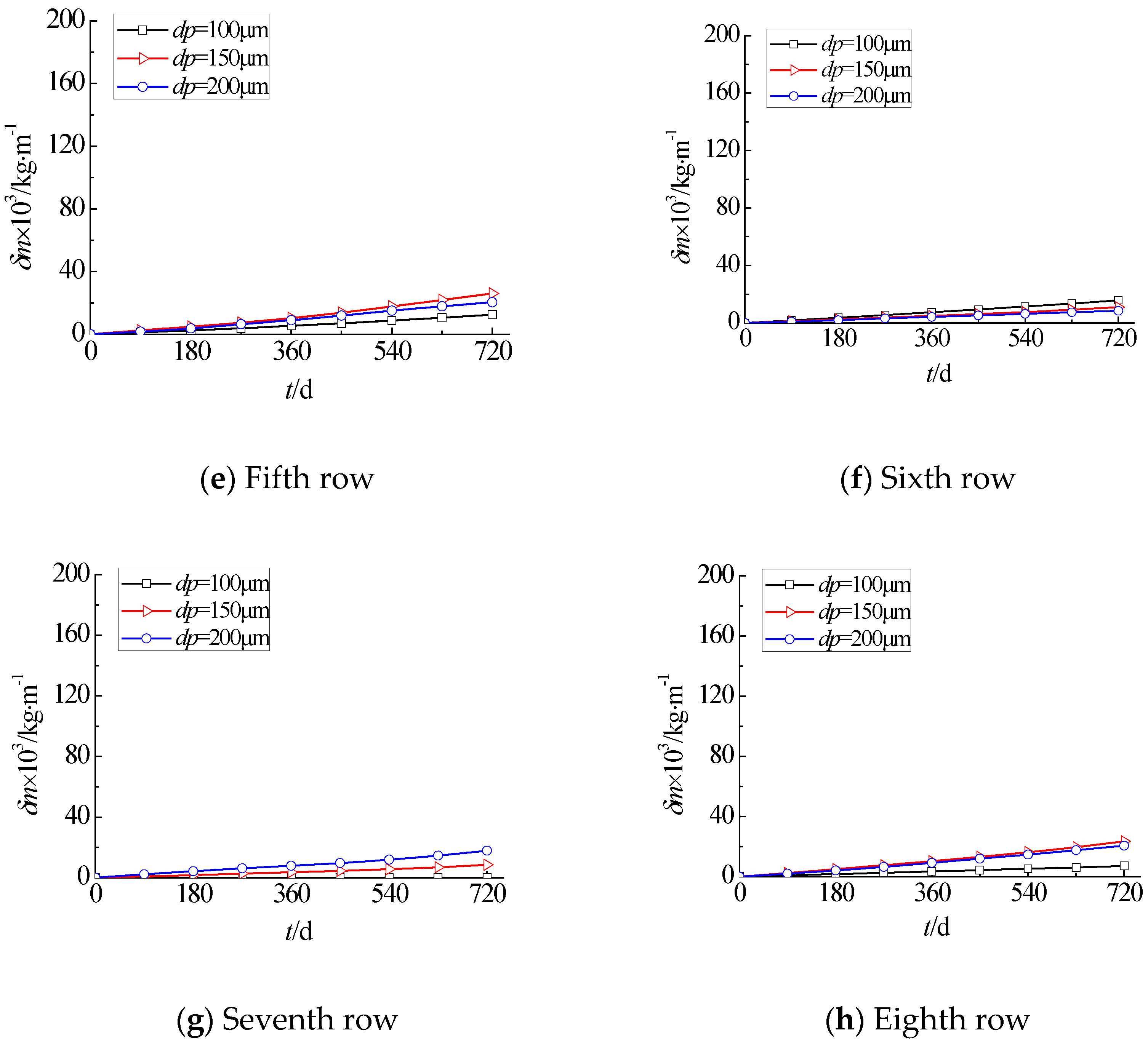
4.1.2. Local Erosion Loss
Figure 10 shows the local erosion loss of different rows under various ash sizes. From this figure, the local erosion loss is consistent with the global erosion loss. The local erosion loss is approximately linear to the working time. The erosion loss of the first row occupies more than half of the global erosion loss. Ash impacts the first rows, and the kinetic energy decreases. Then most of the ash particles follow the gas flow, which hinders the particle collision in the other rows.
Similarly, as the ash size increases, the growth amplification of local erosion loss decreases in the first row. Meanwhile, with the ash size increased, the mass flow of ash impacting the economizer rises in the first row, which raises the probability of particle rebound and collision in other rows (compared with Figure 10a–h). For an ash particle diameter of 200 µm, these rebound phenomena occur in all rows. Second place is 150 µm, and 100 µm is the least. The probability of the particle rebound ultimately influences the growth amplification of global erosion. As the ash size increases to a certain numerical value, the probability of the particle rebound reaches the limit, which leads the growth amplification to decrease.
4.2. Evolution Process of Erosion
4.2.1. Maximum Erosion Depth
Figure 11 shows the maximum erosion depths of the different rows under various ash sizes. The maximum erosion depth is defined as the most critical region, as it represents the thinnest location of the tube wall. From this figure, the maximum erosion depth depends linearly on the working time at the initial time. However, compared to the linear trend (gray dashed line in Figure 11a,b), the growth of the maximum erosion depth slows down gradually. This growing trend forms a favorable flow passage, which prolongs the service life of the economizer effectively.
Since maximum erosion depth in the first row is maximal, this row is the most dangerous and of the greatest concern. Maximum erosion depth of the first row is double or even several times that of other rows. Moreover, not in all rows, the 200 µm ash particle impacts the most powerfully, and the maximum erosion depth is maximal. In the third, fourth, fifth, and eighth row, the maximum is under an ash particle diameter of 150 µm. In the sixth row, the maximum appears under an ash particle diameter of 100 µm. This is mainly caused by particle rebound in the first row, which drives other rows to remove more material as the rebounded particles impact them with different kinetic energies and incidence angles.
4.2.2. Erosion Profile
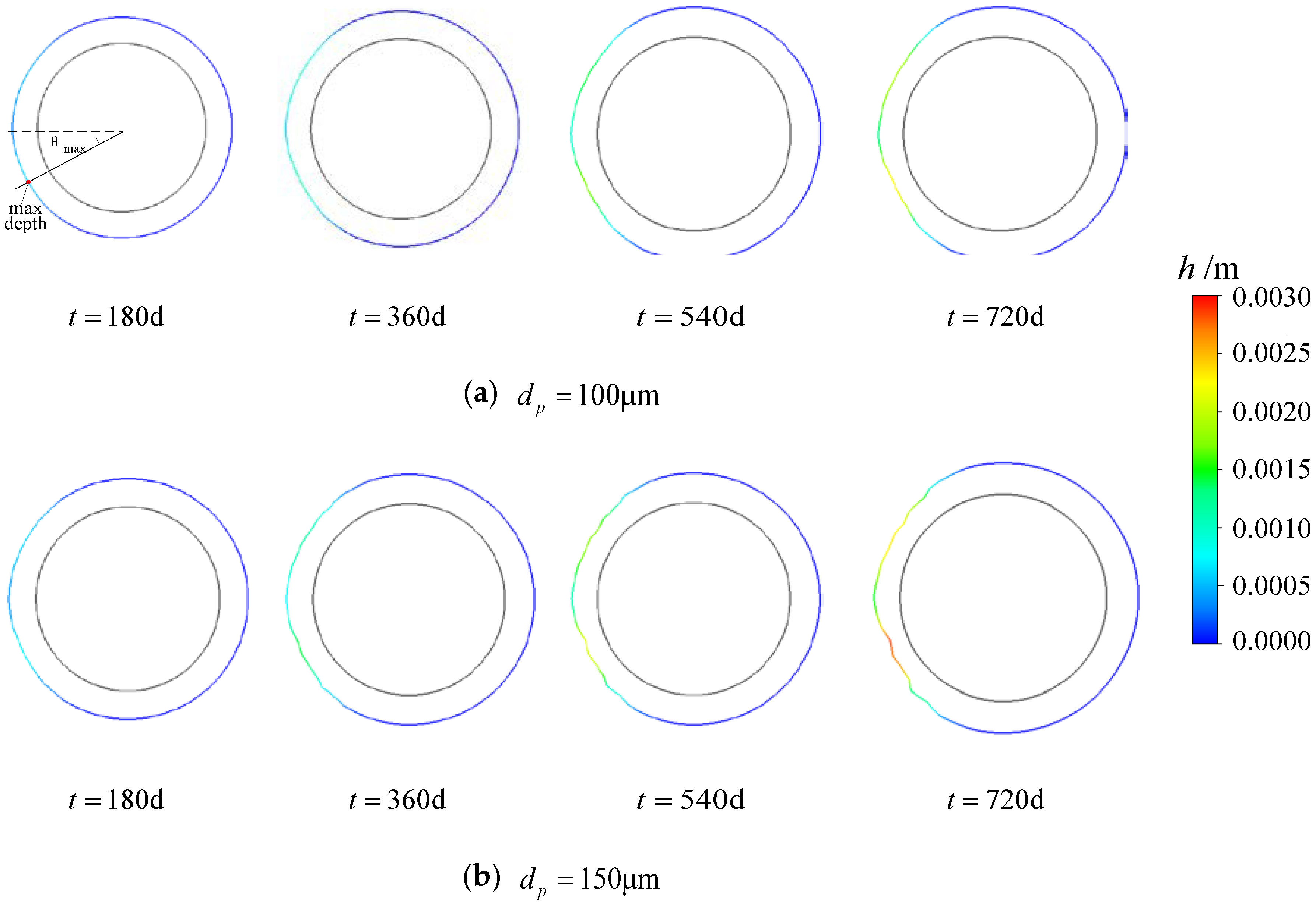
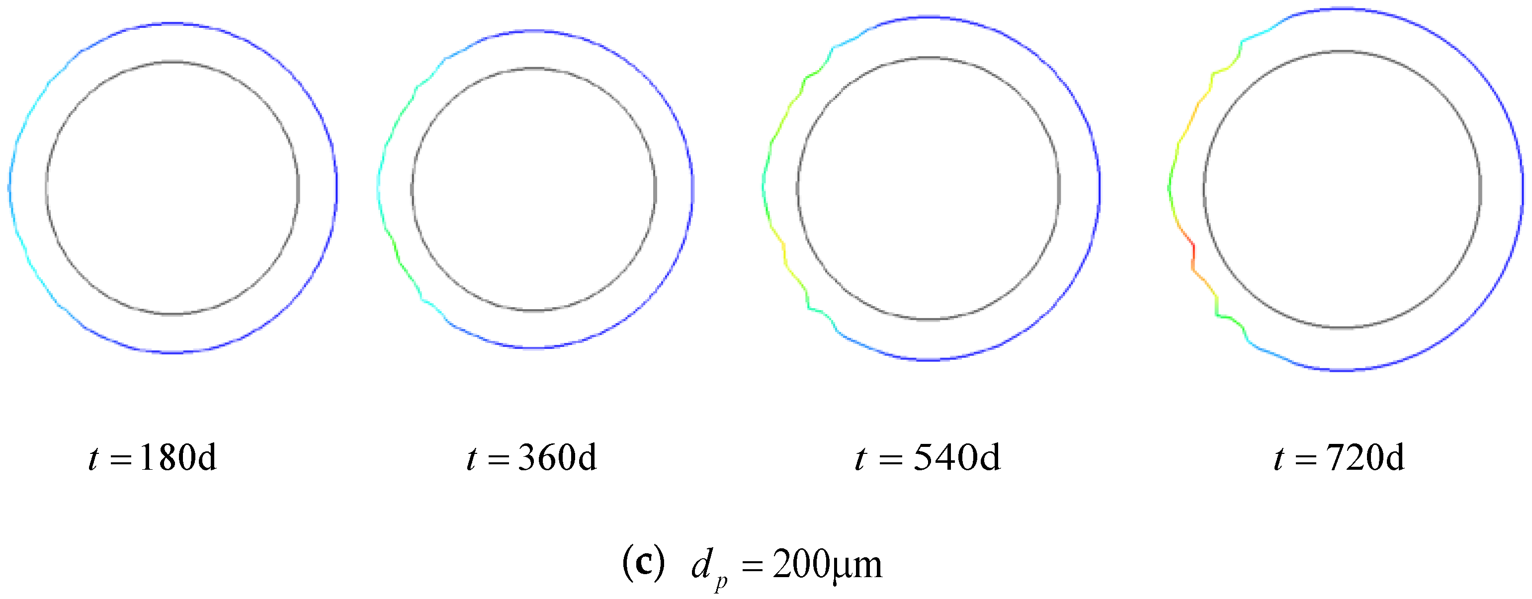
Considering that erosion in the first row is the most serious, this paper focuses on the evolution process of the erosion profile for the first row. Figure 12 shows the evolution process of the erosion profile with different ash sizes in the first row. From this figure, as time proceeds, a “V-shape” is gradually formed, which is similar to the erosion profile in Figure 1. This confirms that the dynamic mesh technology is advisable to describe the erosion of economizer tubes.
In addition, θ is introduced as the angle between the position of the erosion profile and the reverse direction of incoming flow, and θmax represents θ in the location of maximum erosion depth in Figure 12a. From Figure 12, larger ash impacts the first row with a smaller angle of θmax. As mentioned earlier, larger ash has greater inertia and less motion, ensuring that the location of the maximum erosion rate appears with a smaller θ.
4.3. Evolution Process of Particle Motion
Figure 13 shows the particle motion from the specific position in the inlet. From this figure, the particle collision point obviously moves to the center of the economizer tube over time. Meanwhile, due to more material loss with a larger particle, the larger particle moves across a longer distance. In order to describe the particle motion along the radial and tangential direction, Figure 14 is adopted to illustrate the collision point trajectory from the specific position in the inlet, which is the top view of Figure 13a. From this figure, with time increasing, the collision point trajectory moves along the increasing direction of the absolute value of θ. Just because of this, the probabilities of impingement and the growth of the maximum erosion depth slow down gradually in later stages. Although the trend of erosion loss is unlike the maximum erosion depth after 2 years, the erosion loss based on this result is predicted to slowly increase in the future.
4.4. Expiry Periods
In Figure 11a, the safe region is defined as the value below 1.99 mm (equal to the critical value of 4.01 mm in wall thickness [25], which is the minimum wall thickness by the specific theoretical calculation). When the maximum erosion depth is up to 1.99 mm, the first row of the economizer tube easily bursts. From this figure, the expiry periods are respectively 710, 530, and 440 days with 100 µm, 150 µm, and 200 µm. These data indicate the expiry period is shortened as the ash diameter increases. Moreover, as the ash size increases, the declining amplification of expiry periods is retarded.
5. Conclusions
The present research aims to investigate a novel method for the solution of the evolution process and its applications to the expiry period of an economizer bank. The CFD-DPM approach coupled with the UDF of the erosion model and the dynamic mesh technology is utilized to solve this complex issue. Based on the results of the applications, the following conclusions are made:
- (1)
- The CFD-DPM approach coupled with the UDF of Huang’s erosion model and the dynamic mesh technology can describe the evolution process of erosion on an economizer bank, especially the erosion profile; by comparing the simulation results with the erosion profile on-site, the correctness is verified for this proposed CFD-DPM approach.
- (2)
- The global/local erosion loss and the maximum erosion depth are linearly related to the working time, but the growth of the maximum erosion depth slows down gradually in the later stage; as the ash size increases, the growth amplification of global erosion loss, local erosion in the first row, and the maximum erosion depth decrease.
- (3)
- With increasing time, the collision point trajectory moves along the increasing direction of the absolute value of θ in the first row, which explains why the growth of the maximum erosion depth slows down in later stages.
- (4)
- The expiry period is shortened as the ash diameter increases; moreover, as the ash size increases, the declining amplification of expiry periods is retarded.
Author Contributions
F.S. and X.J. led the project and coordinated the study; Y.D., C.Y. and B.Z. conducted the modelling analysis; Y.D. and Z.Q. conducted the numerical simulation. C.Y. participated in the data analysis. Y.D. and C.Y. prepared, and Z.Q. edited the manuscripts; Y.D. coordinated the manuscript submission. All authors read and approved the final manuscript.
Funding
This research was funded by the National Natural Science Fund Program of China, grant number No. 51706043, and the Jiangsu Natural Science Foundation, grant number No. BK20170679.
Acknowledgments
Research was supported by Datang Nanjing Environmental Protection Technology Co., Ltd. Without the support, this work would not have been possible.
Conflicts of Interest
The authors declare no conflict of interest.
Nomenclature
| area of grid element [m2] | model constant | ||
| model constant | fluid thermal conductivity [W/(m·K)] | ||
| model constant | Knudsen number | ||
| model constant | particle mass [kg] | ||
| model constant | gas pressure [pa] | ||
| drag coefficient | Reynolds number | ||
| model constant | turbulence kinetic energy source term [kg/(m·s3)] | ||
| specific heat [J/(kg·K)] | turbulence dissipation rate source term [kg/(m·s4)] | ||
| model constant | gas temperature [K] | ||
| model constant | gas velocity vector [m/s] | ||
| model constant | gas velocity of i-direction [m/s] | ||
| deformation tensor | particle velocity vector [m/s] | ||
| particle diameter [m] | the coordinate of i-direction [m] | ||
| model constant | particle velocity magnitude [m/s] | ||
| total energy [J/kg] | gas velocity magnitude [m/s] | ||
| normal coefficient of velocity restitution | contribution of the fluctuating dilatation in compressible turbulence to the overall dissipation rate [kg/(m·s3)] | ||
| tangential coefficient of velocity restitution | incidence angle | ||
| ratio of abrasion loss and particle mass [g/kg] | gas density [kg/m3] | ||
| drag force [N] | density of economizer material [kg/m3] | ||
| gravity [N] | particle density [kg/m3] | ||
| thermophoretic force [N] | Gas stress tensor [pa] | ||
| Saffman lift force [N] | Kronecker tensor | ||
| acceleration of gravity [m/s2] | erosion loss [kg/m] | ||
| generation of turbulence kinetic energy due to buoyancy [kg/(m·s3)] | time interval [s] | ||
| generation of turbulence kinetic energy due to the velocity gradients [kg/(m·s3)] | gas viscosity [pa·s] | ||
| h | erosion depth [mm] | gas second viscosity [pa·s] | |
| hi,j | erosion depth of grid element [mm] | turbulent Prandtl number for k | |
| particle thermal conductivity [W/(m·K)] | turbulent Prandtl number for ε |
References
- Arabnejad, H.; Mansouri, A.; Shirazi, S.A.; McLaury, B.S. Abrasion erosion modeling in particulate flow. Wear 2017, 376–377, 1194–1199. [Google Scholar] [CrossRef]
- Alam, T.; Farhat, Z.N. Slurry erosion surface damage under normal impact for pipeline steels. Eng. Fail. Anal. 2018, 90, 116–128. [Google Scholar] [CrossRef]
- Eichner, D.; Schlieter, A.; Leyens, C.; Shang, L.; Shayestehaminzadeh, S.; Schneider, J.M. Solid particle erosion behavior of nanolaminated Cr2AlC films. Wear 2018, 402–403, 187–195. [Google Scholar] [CrossRef]
- Ji, X.; Wu, J.; Pi, J.; Cheng, J.; Shan, Y.; Zhang, Y. Slurry erosion induced surface nanocrystallization of bulk metallic glass. Appl. Surf. Sci. 2018, 440, 1204–1210. [Google Scholar] [CrossRef]
- William, L. Failure analysis on the economisers of a biomass fuel boiler. Eng. Fail. Anal. 2013, 31, 101–117. [Google Scholar] [CrossRef]
- Finnie, I. Erosion of surfaces. Wear 1960, 3, 87–103. [Google Scholar] [CrossRef]
- Finnie, I. Some reflections on the past and future of erosion. Wear 1995, 186–187, 1–10. [Google Scholar] [CrossRef]
- Bitter, J. A study of erosion phenomena Part I. Wear 1963, 6, 5–21. [Google Scholar] [CrossRef]
- Bitter, J. A study of erosion phenomena Part II. Wear 1963, 6, 169–190. [Google Scholar] [CrossRef]
- Huang, C.; Chiovelli, S.; Minev, P.; Luo, J.; Nandakumar, K. A comprehensive phenomenological model for erosion of materials in jet flow. Powder Technol. 2008, 187, 273–279. [Google Scholar] [CrossRef]
- Grant, G.; Tabakoff, W. An Experimental Investigation of the Erosion Characteristics of 2024 Aluminum Alloy; Report; Cincinnati University: Cincinnati, OH, USA, 1973; p. 49. [Google Scholar]
- Oka, Y.I.; Okamura, K.; Yoshida, T. Practical estimation of erosion damage caused by solid particle impact: Part 1: Effects of impact parameters on a predictive equation. Wear 2005, 259, 95–101. [Google Scholar] [CrossRef]
- Oka, Y.I.; Yoshida, T. Practical estimation of erosion damage caused by solid particle impact: Part 2: Mechanical properties of materials directly associated with erosion damage. Wear 2005, 259, 102–109. [Google Scholar] [CrossRef]
- Haugen, K.; Kvernvold, O.; Ronold, A.; Sandberg, R. Sand erosion of wear-resistant materials: Erosion in choke valves. Wear 1995, 186–187, 179–188. [Google Scholar] [CrossRef]
- Ahlert, K. Effects of Particle Impingement Angle and Surface Wetting on Solid Particle Erosion of AISI 1018 Steel. Master’s. Thesis, The University of Tulsa, Tulsa, OK, USA, 1994. [Google Scholar]
- McLaury, B.S. Predicting Solid Particle Erosion Resulting from Turbulent Fluctuations in Oilfield Geometries. Ph.D. Thesis, The University of Tulsa, Tulsa, OK, USA, 1996. [Google Scholar]
- Zhang, Y.; Reuterfors, E.P.; McLaury, B.S.; Shirazi, S.A.; Rybicki, E.F. Comparison of computed and measured particle velocities and erosion in water and air flows. Wear 2007, 263, 330–338. [Google Scholar] [CrossRef]
- Shamshirband, S.; Malvandi, A.; Karimipour, A.; Goodarzi, M.; Afrand, M.; Petković, D.; Dahari, M.; Mahmoodian, N. Performance investigation of micro- and nano-sized particle erosion in a 90° elbow using an ANFIS model. Powder Technol. 2015, 284, 336–343. [Google Scholar] [CrossRef]
- Moakhar, R.S.; Mehdipour, M.; Ghorbani, M.; Mohebali, M.; Koohbor, B. Investigations of the failure in boilers economizer tubes used in power plants. J. Mater. Eng. Perform. 2013, 22, 2691–2697. [Google Scholar] [CrossRef]
- Ding, Q.; Tang, X.F.; Yang, Z.G. Failure analysis on abnormal corrosion of economizer tubes in a waste heat boiler. Eng. Fail. Anal. 2017, 73, 129–138. [Google Scholar] [CrossRef]
- Yang, L. One-fluid formulation for fluid–structure interaction with free surface. Comput. Methods Appl. Mech. Eng. 2018, 332, 102–135. [Google Scholar] [CrossRef]
- Joshson, A.A. Dynamic-mesh CFD and its application to flapping-wing micro-air vehicles. In Proceedings of the 25th Army Science Conference, Orlando, FL, USA, 27–30 November 2006; ANSI: Orlando, FL, USA, 2006. [Google Scholar]
- Savidis, S.A.; Aubram, D.; Rackwitz, F. Arbitrary Lagrangian-eulerian finite element formulation for geotechnical construction processes. J. Theor. Appl. Mech. 2008, 38, 165–194. [Google Scholar]
- Li, J.; Hesse, M.; Ziegler, J.; Woods, A.W. An arbitrary Lagrangian Eulerian method for moving-boundary problems and its application to jumping over water. J. Comput. Phys. 2005, 208, 289–314. [Google Scholar] [CrossRef]
- Yuping, C. Boiler Instruction Manual of DAIHAI in China; Shang Boiler Works, Ltd.: Shanghai, China, 2006. [Google Scholar]
- Versteeg, H.; Malalasekera, W. An Introduction to Computational Fluid Dynamics: The Finite Volume Method; Prentice Hall: London, UK, 1995. [Google Scholar]
- Gao, W.; Li, Y.; Kong, L. Numerical investigation of erosion of tube sheet and tubes of a shell and tube heat exchanger. Comput. Chem. Eng. 2017, 96, 115–127. [Google Scholar] [CrossRef]
- Launder, B.E.; Spalding, D.B. The numerical computation of turbulent flows. Comput. Methods Appl. Mech. Eng. 1974, 3, 269–289. [Google Scholar] [CrossRef]
- ANSYS. Ansys Fluent User’s Guide; Ansys Inc.: Canonsburg, PA, USA, 2015. [Google Scholar]
- Grant, G.; Tabakoff, W. Erosion Prediction in Turbomachinery Resulting from environmental solid particles. J. Aircr. 1975, 12, 471–478. [Google Scholar] [CrossRef]
- ASTM. Standard test method for conducting erosion tests by solid particle impingement. ASTM Int. 2013. [Google Scholar] [CrossRef]
- Sagayaraj, T.A.D.; Suresh, S.; Chandrasekar, M. Experimental studies on the erosion rate of different heat treated carbon steel economizer tubes of power boilers by fly ash particles. Int. J. Miner. Metall. Mater. 2009, 16, 534–539. [Google Scholar] [CrossRef]
Figure 1.
Particle erosion. (a) SCR catalyst; (b) economizer (reprinted with permission from reference [5]. Copyright 2018 ELSEVIER).
Figure 1.
Particle erosion. (a) SCR catalyst; (b) economizer (reprinted with permission from reference [5]. Copyright 2018 ELSEVIER).

Figure 2.
Calculativeprocess of erosion evolution.

Figure 3.
Erosion profile calculation with dynamic mesh: (a) before collision; (b) after collision.

Figure 4.
Schematic diagram of the economizer tube bank.

Figure 5.
Three-dimensional diagram of the economizer unit.

Figure 6.
Grid refinement of the tube wall.

Figure 7.
Erosion curve of impact angle on SA 210GrA1.

Figure 8.
Erosion curve of ash size on SA 210GrA1.

Figure 9.
Global erosion loss under different ash sizes.

Figure 10.
Local erosion loss under different ash sizes.


Figure 11.
Maximum erosion depth under different ash sizes.


Figure 12.
Evolution process of erosion profile in the first row.


Figure 13.
Particle motion.


Figure 14.
Collision point trajectory ().


Table 1.
Structural parameters of the economizer tube [25].
Table 1.
Structural parameters of the economizer tube [25].
| Material | Rows | Diameter/mm | Transversal Pitch a/mm | Longitudinal Pitch b1/mm | Longitudinal Pitch b2/mm |
|---|---|---|---|---|---|
| SA 210 GrA1(N) | 135 | Φ51×6 | 144 | 102 | 69 |
© 2018 by the authors. Licensee MDPI, Basel, Switzerland. This article is an open access article distributed under the terms and conditions of the Creative Commons Attribution (CC BY) license (http://creativecommons.org/licenses/by/4.0/).
Share and Cite
MDPI and ACS Style
Dong, Y.; Qiao, Z.; Si, F.; Zhang, B.; Yu, C.; Jiang, X. A Novel Method for the Prediction of Erosion Evolution Process Based on Dynamic Mesh and Its Applications. Catalysts 2018, 8, 432. https://doi.org/10.3390/catal8100432
AMA Style
Dong Y, Qiao Z, Si F, Zhang B, Yu C, Jiang X. A Novel Method for the Prediction of Erosion Evolution Process Based on Dynamic Mesh and Its Applications. Catalysts. 2018; 8(10):432. https://doi.org/10.3390/catal8100432
Chicago/Turabian StyleDong, Yunshan, Zongliang Qiao, Fengqi Si, Bo Zhang, Cong Yu, and Xiaoming Jiang. 2018. "A Novel Method for the Prediction of Erosion Evolution Process Based on Dynamic Mesh and Its Applications" Catalysts 8, no. 10: 432. https://doi.org/10.3390/catal8100432
Note that from the first issue of 2016, this journal uses article numbers instead of page numbers. See further details here.