A 2-D model for Intermediate Temperature Solid Oxide Fuel Cells Preliminarily Validated on Local Values

Abstract

Intermediate Temperature Solid Oxide Fuel Cell (IT-SOFC) technology offers interesting opportunities in the panorama of a larger penetration of renewable and distributed power generation, namely high electrical efficiency at manageable scales for both remote and industrial applications. In order to optimize the performance and the operating conditions of such a pre-commercial technology, an effective synergy between experimentation and simulation is fundamental. For this purpose, starting from the SIMFC (SIMulation of Fuel Cells) code set-up and successfully validated for Molten Carbonate Fuel Cells, a new version of the code has been developed for IT-SOFCs. The new release of the code allows the calculation of the maps of the main electrical, chemical, and physical parameters on the cell plane of planar IT-SOFCs fed in co-flow. A semi-empirical kinetic formulation has been set-up, identifying the related parameters thanks to a devoted series of experiments, and integrated in SIMFC. Thanks to a multi-sampling innovative experimental apparatus the simultaneous measurement of temperature and gas composition on the cell plane was possible, so that a preliminary validation of the model on local values was carried out. A good agreement between experimental and simulated data was achieved in terms of cell voltages and local temperatures, but also, for the first time, in terms of local concentration on the cell plane, encouraging further developments. This numerical tool is proposed for a better interpretation of the phenomena occurring in IT-SOFCs and a consequential optimization of their performance.

1. Introduction

With the increase of pollution resulting from the use of fossil fuels, a significant effort in the research and development of alternative fuels is aimed at all countries on a worldwide level. Among the alternative technologies to produce power with low emissions, fuel cells play a key role in this scenario. Nowadays high-temperature fuel cells such as Molten Carbonate Fuel Cells (MCFCs) and Solid Oxide Fuel Cells (SOFCs) are under study in order to be introduced into the world market. In particular, the latter technology presents several advantages with respect to internal combustion engines such as high efficiency, fuel flexibility, and a reduced environmental impact. SOFCs have been the subject of study since the first years of the 1937 by Reference [1]. During the 1970s and 1980s, support for the development of SOFCs came from large generating equipment manufacturers such as Westinghouse, ABB, and General Electric Company Plc. From the mid-1990s to the present, several other cell designs and materials have been explored in order to reduce the operating temperature [2], provided the internal resistance of the cell and the electrode kinetics were adequate and internal reforming could be carried out. Specifically, anode-supported planar Intermediate Temperature Solid Oxide Fuel Cells (IT-SOFCs) became quite popular thanks to performance and cost consideration factors [3].

These devices can be applied in several sectors such as:

• portable applications (power less than 1 kW);
• the naval and automotive sector (power output between 1 and 250 kW);
• distributed generation of power (power output until 10 MW).

IT-SOFCs work in a range of temperatures between 923 and 1023 K [4], so that their waste heat can be reutilised in cogeneration systems [5].

Nevertheless, a further technological improvement is necessary to promote an extensive industrial commercialization. For this reason, a synergy between experimentation and simulation is proposed here as the better approach to evaluate and optimise performance, providing solutions for diagnostic, predictive and development issues.

In recent years, a good number of scientists have investigated into SOFC modelling to estimate physical, chemical and kinetic key performance indicators and have carefully followed the scale-up from a lab-scale to an industrial one. These models range from zero-dimensional (0-D) ones, which are lumped models using concentrated parameters and which can only relate to cell global proprieties, to three dimensional (3-D) ones, which are detailed models using distributed parameters and can describe cell local proprieties on the three spatial coordinates. The use of any one of these types of models depends of the research aims: Usually 3-D and 2-D models concern phenomena investigation, while 1-D and 0-D models are related to control purposes [6,7,8,9,10,11].

In particular, with 3-D models, the attention is focused on the local behaviour providing temperature and component distribution along the three coordinates so as, for example, in References [12,13,14,15]. Detailed 3D models are usually very computationally expensive due to the highly coupled and nonlinear nature of their mathematical formulation as well as a large number of functional domains in the cell. In order to simplify the mathematical and computational complexity, the cell geometry is usually assumed to be 2-D [16,17,18,19,20,21,22], representing a 2-D cross-sectional domain and neglecting the changes of physics in the third coordinate.

On the other hand, sometimes lower dimensional models are used in the study of dynamic or complex systems because of their minor computational effort with respect to the high dimensional ones, although at the expense of less reliability of the resulting predictions.

In the 1-D model, the profiles of the chemical-physical properties are calculated only along the more significant coordinate, so that two of the geometrical dimensions are neglected [23,24,25,26,27,28]. Finally, 0-D models are based on groups of algebra equations to calculate for example cell voltage, power output, and cell efficiency using a simplified macroscopic approach, effective, for example, for control purposes [29].

The mentioned models can be defined “white” models, because they are based on explicit physical equations, or at least “grey” models, when based on a semi-empirical approach which integrates a priori knowledge of the physical process and mathematical relations that describe the behavior of the system. In the latter case, the model construction foresees at first the set-up of the basic model, then the conduction of experimental tests, finally the calibration and validation of the model on the basis of the experimental results. An example of this approach can be found in the work by Sorrentino and Pianese [30] for the diagnosis of a SOFC unit in a complex system. Nevertheless, in addition to these first principle models, “black-box” models have also been developed as behavioral models derived through a statistical data-driven approach. As opposed to the physical models, they are not based on explicit physical equations, but on a database of measured experimental values that are capable of reflecting the relationship between inputs and outputs, of which examples can be found in References [31,32,33,34,35,36].

In the present work, a simplified semi-empirical electro-kinetic relationship is proposed for IT-SOFCs, starting from physical principles and performing devoted experimental tests for the identification of the parameters. The kinetic expression has been integrated as a new kinetic core in the SIMFC code. It is a numerical 2-D deterministic model, based on local mass, energy, charge, and momentum balances, which have been set-up and successfully validated by PERT (Process Engineering Research Team) of the University of Genoa for Molten Carbonate Fuel Cells [37,38,39] and has been updated to allow also IT-SOFCs simulation. The experimental tests have been carried out on planar single cells at ENEA laboratories of the Casaccia Research Centre. Thanks to an innovative experimental facility [40], it has been possible to also validate, experimentally, the local values of temperature and anodic composition calculated on the cell plane. The last point presents a new interesting contribution to the research in this field. Both theoretical and experimental results are reported and discussed in the following sections.

2. Modelling

2.1. Semi-Empirical Kinetics

If we fed hydrogen to the anode and oxygen to the cathode, the reactions that occur at the IT-SOFC electrodes are the following:

$${\mathrm{H}}_2+{\mathrm{O}}^{2-}\to {\mathrm{H}}_2\mathrm{O}+2{\mathrm{e}}^{-}\mathrm{Anode}$$

(1)

$$\frac{1}{2}{\mathrm{O}}_2+2{\mathrm{e}}^{-}\to {\mathrm{O}}^{2-}\mathrm{Cathode}$$

(2)

following a thermodynamic approach [37], the equilibrium cell voltage $\Delta \mathrm{E}$ can be expressed by means of the Nernst equation:

$$\Delta \mathrm{E}={\mathrm{E}}_{\mathrm{an}}-{\mathrm{E}}_{\mathrm{cat}}={\mathrm{E}}_0+\frac{\mathrm{R}\mathrm{T}}{2\mathrm{F}}\ln \frac{{\mathrm{p}}_{{\mathrm{H}}_2}{\mathrm{p}}_{{\mathrm{O}}_2}^{1/2}}{{\mathrm{p}}_{{\mathrm{H}}_2\mathrm{O}}}$$

(3)

where R is the universal gas constant and F is the Faraday constant.

${\mathrm{E}}_0$ is the reversible cell voltage, which can be expressed as a function of temperature using this relationship [41]:

$${\mathrm{E}}_0=1.253-2.4516{10}^{-4}\mathrm{T}$$

(4)

Analysing the problem from a kinetic point of view, under load the operating cell voltage $\Delta \mathrm{V}$ is penalized by polarizations, which can be considered as follows:

$$\Delta \mathrm{V}=\Delta \mathrm{E}-{\mathsf{\eta }}_{\mathrm{Ohm}}-{\mathsf{\eta }}_{\mathrm{an}}-{\mathsf{\eta }}_{\mathrm{cat}}$$

(5)

where η_Ohm is the voltage loss due to the purely Ohmic internal resistance as well as the contact resistance, η_anode and η_cathode are the polarizations at the electrode scale due to activation and reactant diffusion phenomena.

In this paper, working at sufficiently low fuel utilization factors, that is ratios between reacted hydrogen and fed hydrogen lower than 30%, the characteristic curves results are quite linear and Equation (5) has been simplified assuming:

$$\Delta \mathrm{V}=\Delta \mathrm{E}-{\mathrm{R}}_{\mathrm{tot}}$$

(6)

where

$${\mathrm{R}}_{\mathrm{tot}}={\mathrm{R}}_{\mathrm{Ohm}}+{\mathrm{R}}_{\mathrm{an}}+{\mathrm{R}}_{\mathrm{cat}}$$

(7)

Ohmic resistance ${\mathrm{R}}_{\mathrm{Ohm}}$ can be evaluated by means of a temperature dependent relationship

$${\mathrm{R}}_{\mathrm{ohm}}={\mathrm{P}}_0+{\mathrm{P}}_1\mathrm{T}\exp \left(\frac{{\mathrm{P}}_2}{\mathrm{T}}\right)$$

(8)

where P₀ represents the contact resistance, usually negligible [42,43,44], while P₁ and P₂ are phenomenological coefficients evaluated by fitting experimental data.

The electrode polarizations have been derived from the Butler-Volmer equation [37]

$$\mathrm{j}={\mathrm{j}}_0\left[{\exp }^{(2\mathrm{F}\mathsf{\eta }/\mathrm{RT})}{\displaystyle \prod }_{\mathrm{i}}\frac{{\mathrm{c}}_{\mathrm{isur}}^{{\mathsf{\alpha }}_{\mathrm{i}}^{\prime }}}{{\mathrm{c}}_{\mathrm{i}}^{{\mathsf{\alpha }}_{\mathrm{i}}^{\prime }}}-{\exp }^{(2\mathrm{F}\mathsf{\eta }/\mathrm{RT})}{\displaystyle \prod }_{\mathrm{i}}\frac{{\mathrm{c}}_{\mathrm{isur}}^{{\mathsf{\alpha }}_{\mathrm{i}}^{″}}}{{\mathrm{c}}_{\mathrm{i}}^{{\mathsf{\alpha }}_{\mathrm{i}}^{″}}}\right]$$

(9)

when the reverse reaction, diffusion phenomena and non-linear terms are neglected.

In terms of electrode resistances ${\mathrm{R}}_{\mathrm{an}}$ and ${\mathrm{R}}_{\mathrm{cat}}$, it can be obtained:

$${\mathrm{R}}_{\mathrm{an}\left(\mathrm{or}\mathrm{cat}\right)}\cong \frac{\mathrm{RT}}{2\mathrm{F}{\mathrm{j}}_{0,\mathrm{an}\left(\mathrm{or}\mathrm{cat}\right)}}$$

(10)

where ${\mathrm{j}}_0$ is the exchange current density which can be expressed as follows [45]:

$${\mathrm{j}}_{0,\mathrm{an}}=\mathrm{A}{\left(\frac{{\mathrm{p}}_{{\mathrm{H}}_2}}{{\mathrm{p}}_{\mathrm{ref}}}\right)}^{\mathrm{B}}{\left(\frac{{\mathrm{p}}_{{\mathrm{H}}_2\mathrm{O}}}{{\mathrm{p}}_{\mathrm{ref}}}\right)}^{\mathrm{C}}\exp \left(-\frac{\mathrm{D}}{\mathrm{T}}\right)$$

(11)

$${\mathrm{j}}_{0,\mathrm{cat}}=\mathrm{L}{\left(\frac{{\mathrm{p}}_{{\mathrm{O}}_2}}{{\mathrm{p}}_{\mathrm{ref}}}\right)}^{\mathrm{M}}\exp \left(-\frac{\mathrm{N}}{\mathrm{T}}\right)$$

(12)

where A, B, C, D, L, M, and N are phenomenological coefficients based on experimental data and/or evaluated by physical equations.

As the reference operating pressure is equal to 1 atm and in the studied operating conditions it is possible to neglect the dependence on water thanks to the low ratio $\frac{{\mathrm{p}}_{{\mathrm{H}}_2\mathrm{O}}}{{\mathrm{p}}_{{\mathrm{H}}_2}}$ [46], it is possible to write:

$${\mathrm{R}}_{\mathrm{an},{\mathrm{H}}_2}=\frac{{\mathrm{P}}_3\mathrm{R}\mathrm{T}{\exp }^{\left(\frac{{\mathrm{P}}_4}{\mathrm{T}}\right)}}{2\mathrm{F}{\left({\mathrm{x}}_{{\mathrm{H}}_2}\right)}^{{\mathrm{P}}_5}}$$

(13)

$${\mathrm{R}}_{\mathrm{cat},{\mathrm{O}}_2}=\frac{{\mathrm{P}}_6\mathrm{R}\mathrm{T}{\exp }^{\left(\frac{{\mathrm{P}}_7}{\mathrm{T}}\right)}}{2\mathrm{F}{\left({\mathrm{x}}_{{\mathrm{O}}_2}\right)}^{{\mathrm{P}}_8}}$$

(14)

Finally, the semi-empirical kinetic formulation for IT-SOFCs is obtained:

$$\Delta \mathrm{V}=\Delta \mathrm{E}-{\mathrm{R}}_{\mathrm{tot}}\mathrm{j}=\Delta \mathrm{E}-\left({\mathrm{P}}_1\mathrm{T}\exp \left(\frac{{\mathrm{P}}_2}{\mathrm{T}}\right)+\frac{{\mathrm{P}}_3\mathrm{R}\mathrm{T}{\exp }^{\left(\frac{{\mathrm{P}}_4}{\mathrm{T}}\right)}}{2\mathrm{F}{\left({\mathrm{x}}_{{\mathrm{H}}_2}\right)}^{{\mathrm{P}}_5}}+\frac{{\mathrm{P}}_6\mathrm{R}\mathrm{T}{\exp }^{\left(\frac{{\mathrm{P}}_7}{\mathrm{T}}\right)}}{2\mathrm{F}{\left({\mathrm{x}}_{{\mathrm{O}}_2}\right)}^{{\mathrm{P}}_8}}\right)\mathrm{j}$$

(15)

where the empirical coefficients P₁, P₂, P₃, P₄, P₅, P₆, P₇ and P₈ must be identified with experimental tests. The physical meanings of the phenomenological parameters quoted previously, is the following:

• P₁ and P₂ are related to the calculation of the fuel cell conductivity;
• P₃, P₄, and P₅ are related to the pre-exponential factor, activation energy and order of anodic reaction of the expression of the linear part of the resistance respectively;
• P₆, P₇, and P₈ are related to the pre-exponential factor, activation energy and order of cathodic reaction of the expression of the linear part of the resistance, respectively.

2.2. SIMFC Code

The above discussed formulation was integrated into the SIMFC code, previously developed for Molten Carbonate Fuel Cells [37]. This modelling tool is based on local mass, energy, momentum, and charge balances and allows the calculation of the maps on the cell plane of the main chemical-physical variables characterising the cell behaviour.

This tool is able to simulate steady state as well as transient conditions, runs quickly, it is written in Fortran language and can be implemented in many commercial software applications for system simulation [47].

In the present work, the general structure of the code has been kept the same as Reference [37], but all the balances have been modified taking into account the reactions occurring in IT-SOFCs. In addition, the data related to the cell configuration and materials were updated for the new technology and the gas co-flow feeding system was set-up, as the SIMFC code had been previously validated for crossflow configuration [48].

The basic equations used are reported in

Table 1. Basic equations of the SIMFC model.

Basic Equations
mass balances	anodic gas $\frac{\partial {\mathrm{n}}_{\mathrm{i}}}{\partial \mathrm{x}}=\frac{\mathrm{j}}{2\mathrm{F}}$
	cathodic gas $\frac{\partial {\mathrm{n}}_{\mathrm{i}}}{\partial \mathrm{x}}=\frac{\mathrm{j}}{4\mathrm{F}}$
energy balances	anodic gas ${{\displaystyle \sum }}_{\mathrm{i}}{\mathrm{n}}_{\mathrm{i}}{\mathrm{c}}_{\mathrm{pi}}\frac{\partial {\mathrm{T}}_{\mathrm{an}}}{\partial \mathrm{x}}={{\displaystyle \sum }}_{\mathrm{i}}\frac{\partial {\mathrm{n}}_{\mathrm{i}}}{\partial \mathrm{x}}{{\displaystyle \int }}_{{\mathrm{T}}_{\mathrm{an}}}^{{\mathrm{T}}_{\mathrm{sol}}}{\mathrm{c}}_{\mathrm{pi}}{\mathrm{dT}}_{\mathrm{an}}+\mathrm{Sh}\left({\mathrm{T}}_{\mathrm{sol}}-{\mathrm{T}}_{\mathrm{an}}\right)$
	cathodic gas ${{\displaystyle \sum }}_{\mathrm{i}}{\mathrm{n}}_{\mathrm{i}}{\mathrm{c}}_{\mathrm{pi}}\frac{\partial {\mathrm{T}}_{\mathrm{cat}}}{\partial \mathrm{x}}={{\displaystyle \sum }}_{\mathrm{i}}\frac{\partial {\mathrm{n}}_{\mathrm{i}}}{\partial \mathrm{x}}{{\displaystyle \int }}_{{\mathrm{T}}_{\mathrm{cat}}}^{{\mathrm{T}}_{\mathrm{sol}}}{\mathrm{c}}_{\mathrm{pi}}{\mathrm{dT}}_{\mathrm{an}}+\mathrm{Sh}\left({\mathrm{T}}_{\mathrm{sol}}-{\mathrm{T}}_{\mathrm{cat}}\right)$
	solid ${\mathrm{S}}_{\mathrm{an}}{\mathrm{h}}_{\mathrm{an}}\left({\mathrm{T}}_{\mathrm{sol}}-{\mathrm{T}}_{\mathrm{an}}\right)+{\mathrm{S}}_{\mathrm{cat}}{\mathrm{h}}_{\mathrm{cat}}\left({\mathrm{T}}_{\mathrm{sol}}-{\mathrm{T}}_{\mathrm{cat}}\right)={\mathrm{Q}}_{\mathrm{cond}}+{\mathrm{Q}}_{\mathrm{reac}}$ where ${\mathrm{Q}}_{\mathrm{cond}}={{\displaystyle \sum }}_{\mathrm{n}}\left({\mathsf{\lambda }}_{\mathrm{n}}{\mathrm{s}}_{\mathrm{n}}\right)\left(\frac{{\partial }^2{\mathrm{T}}_{\mathrm{sol}}}{\partial {\mathrm{x}}^2}+\frac{{\partial }^2{\mathrm{T}}_{\mathrm{sol}}}{\partial {\mathrm{y}}^2}\right)$
momentum balances	anodic gas $\frac{\partial {\mathrm{p}}_{\mathrm{an}}}{\partial \mathrm{x}}={\mathrm{K}}_{\mathrm{an}}\frac{{\mathsf{\mu }}_{\mathrm{an}}{\mathsf{\nu }}_{\mathrm{an}}}{{\mathrm{d}}^2}$
	cathodic gas $\frac{\partial {\mathrm{p}}_{\mathrm{cat}}}{\partial \mathrm{x}}={\mathrm{K}}_{\mathrm{cat}}\frac{{\mathsf{\mu }}_{\mathrm{cat}}{\mathsf{\nu }}_{\mathrm{cat}}}{{\mathrm{d}}^2}$
local thermodynamic	nernst voltage $\Delta \mathrm{E}={\mathrm{E}}_{\mathrm{an}}-{\mathrm{E}}_{\mathrm{cat}}={\mathrm{E}}_0+\frac{\mathrm{RT}}{2\mathrm{F}}\ln \frac{{\mathrm{p}}_{{\mathrm{H}}_2}{\mathrm{p}}_{{\mathrm{O}}_2}^{1/2}}{{\mathrm{p}}_{{\mathrm{H}}_2\mathrm{O}}}$
local kinetics	resistance ${\mathrm{R}}_{\mathrm{tot}}={\mathrm{P}}_1\mathrm{Texp}\left(\frac{{\mathrm{P}}_2}{\mathrm{T}}\right)+\frac{{\mathrm{P}}_3\mathrm{R}\mathrm{T}{\exp }^{\left(\frac{{\mathrm{P}}_4}{\mathrm{T}}\right)}}{2\mathrm{F}{\mathrm{p}}_{{\mathrm{H}}_2}{}^{{\mathrm{P}}_5}}+\frac{{\mathrm{P}}_6\mathrm{R}\mathrm{T}{\exp }^{\left(\frac{{\mathrm{P}}_7}{\mathrm{T}}\right)}}{2\mathrm{F}{\mathrm{p}}_{{\mathrm{O}}_2}{}^{{\mathrm{P}}_8}}$
	cell voltage $\Delta \mathrm{V}=\Delta \mathrm{E}-{\mathrm{R}}_{\mathrm{tot}}\mathrm{j}$

. To solve the differential equation system shown in the table, the finite difference method is used with the relaxation method for the energy balance of the solid, which is a Fourier problem.

In particular, the cell plane is divided into an optimised number of sub-cells where balances are applied and where thermodynamic and kinetic proprieties are calculated directly at the local operating conditions.

In this way, for example, Nernst losses [37] due to the varying reactant and product concentration are directly considered thanks to the local approach and so the inaccuracy of combining equilibrium and non-equilibrium statements are avoided [49].

SIMFC needs the following main inputs: average current density (galvanostatic working condition), electro-kinetics parameters, thermodynamic and transport proprieties, composition and total flow rate of the feeding streams, cell geometrical characteristics, and convergence parameters (e.g., number of sub-cells and tolerance values).

The resulting main outputs are: Cell voltage; fuel and oxidant utilisation factors; maps on the cell plane of electrical current densities, Nernst voltage, polarization contributions, temperature (of the solid and gaseous streams), pressure drops, compositions, and flow rates of the gaseous streams.

2.3. Validation Tests

In order to identify the kinetic parameters (P₁–P₈) previously discussed and subsequently validate the local results of the model, a number of experimental tests was carried out as summarized in

Table 2. Test operating conditions.

Conditions	T K	Anode						Cathode
		Flow Rate (10−4 mol s−1)			% mol			Flow Rate (10−4 mol s−1)		% mol
		H2	N2	H2O	H2	N2	H2O	O2	N2	O2	N2
H2 96%	923	11.2	0	0.4	96	0	4	3.8	14.5	21	79
H2 80% (Reference condition)	923	9.3	1.9	0.4	80	16	4	3.8	14.5	21	79
H2 60%	923	7.0	4.2	0.4	60	36	4	3.8	14.5	21	79
H2 40%	923	4.7	6.5	0.4	40	56	4	3.8	14.5	21	79
O2 9%	923	9.3	1.9	0.4	80	16	4	2.1	21.4	9	91
O2 11%	923	9.3	1.9	0.4	80	16	4	2.6	20.9	11	89
O2 13%	923	9.3	1.9	0.4	80	16	4	3.1	20.5	13	87
O2 15%	923	9.3	1.9	0.4	80	16	4	3.5	20.0	15	85
T 948	948	9.3	1.9	0.4	80	16	4	3.8	14.5	21	79
T 973	973	9.3	1.9	0.4	80	16	4	3.8	14.5	21	79
T 998	998	9.3	1.9	0.4	80	16	4	3.8	14.5	21	79

. The experiments have been performed to measure characteristic curves by varying the electric load, maintaining the input constant molar flow rates, and guaranteeing a low reactant utilization factor to avoid diffusion limits.

The temperature and reactant composition have been changed one at a time (with N₂ balancing) in order to isolate their effect on the electrochemical model.

All experiments were carried out at atmospheric pressure.

3. Results and Discussion

3.1. Experimental Data

In Figure 1 the data obtained at the operating conditions named H₂ 96%, H₂ 80%, H₂ 60%, and H₂ 40% (see Table 2) are reported: as expected the performance improves when the content of hydrogen in the anodic flow rate increases. From the characteristic curves, the voltage trend can be evaluated, while the Electrochemical Impedance Spectra (EIS) spectra show two main points: these two intercept with the x-axis of the Nyquist plot. The first one identifies the Ohmic resistance and it is not affected by the composition change. Due to the measurement procedure used, this evaluation does not take into account the contact resistance, nevertheless it has been assumed to be negligible as was previously mentioned [42,43,44]. The second intercept, related to the amplitude of the curve, gives a measure of the decreasing of the sum of Ohmic and polarization resistances when a richer anodic flow rate is fed in.

Similar considerations can be made observing the data obtained varying the feeding concentration of the cathodic reactant (see Figure 2).

Finally, Figure 3 shows the results obtained varying the operating temperature. The improving performances at a higher temperature confirm how the total resistance decreases when temperature increases. The same trend is clearly shown by the EIS spectra. In this case, the Ohmic resistance also varies, assuming high values at high temperatures.

3.2. Parameter Identification

The above discussed experimental data have been used to identify the parameters necessary to calculate the local total resistance R_tot according to the kinetic formulation of Equation (15).

Considering the Ohmic contribution, neglecting the contac losses P₀, the parameters P₁ and P₂ were identified by means of the OriginLab^© software (version 8, OriginLab Corporation, Northampton, MA USA), and the experimental data collected thanks to the EIS analyses at different operating conditions.

Table 3. Values of P₁ and P₂ (Equation (8) of Ohmic resistance) from data fitting and literature.

Parameter	Data Fitting	Ref. [43]	Ref. [42]
P1 [Ohm cm2 K−1]	2 × 10−9	6.34 × 10−7	1.72 × 10−9
P2 [K]	10,986	5210	11,024

compares the obtained results and some literature values: The orders of magnitude are the same.

Regarding the other terms of the Equation (15), namely ${\mathrm{R}}_{\mathrm{an},{\mathrm{H}}_2}$_, and ${\mathrm{R}}_{\mathrm{cat},{\mathrm{O}}_2}$, the parameters have been identified thanks to the above discussed characteristic curves. In particular, this procedure has been followed:

• The slope of the curves has been calculated and interpreted as a global resistance;
• The Nernst loss due to the reactant consumption under different loads has been calculated assuming a linear dependence on current density [37];
• The local total resistance R_tot has been calculated subtracting the Nernst loss from the global resistance;
• The sum of the contributions ${\mathrm{R}}_{\mathrm{an},{\mathrm{H}}_2}$ and ${\mathrm{R}}_{\mathrm{cat},{\mathrm{O}}_2}$ have been obtained by subtracting the Ohmic contribution from the local total resistance;
• P₃ and P₆ have been obtained by using the resulting values of ${\mathrm{R}}_{\mathrm{an},{\mathrm{H}}_2}$ + ${\mathrm{R}}_{\mathrm{cat},{\mathrm{O}}_2}$.

It can be noted that, referring to similar kinetic formulation in the literature, the equivalent parameters, which can be found present in the same orders of magnitude (

Table 4. Values of P₃ and P₆ (Equation (15) of total resistance) from data fitting and literature.

Parameter	Data Fitting	Ref. [45]	Ref. [42]	Ref. [50]	Ref. [51]
P3 [A cm−2]	3.65 × 109	1.34 × 1010	1.68 × 109	5 × 109	1.4 × 1010
P6 [A cm−2]	1.49 × 1010	2.05 × 109	4.76 × 1010	2 × 109	-

). Regarding P₄ and P₇ we chose to use 13230 K [52] and 14433 K [51], respectively, taking them from literature as related to the activation energies of the occurring reactions.

Finally, both P₅ and P₈, have been assumed equal to 0.5, as provided in References [46,53].

The characteristic curves presented above, have been simulated with the SIMFC code using the identified kinetic parameters. As a systematic error of about 0.018 V has been observed in the open circuit comparing the experimental voltage and the theoretical one calculated with the Nernst equation, this correction has been forced in the SIMFC code (subtracting 0.018 V to the theoretical value).

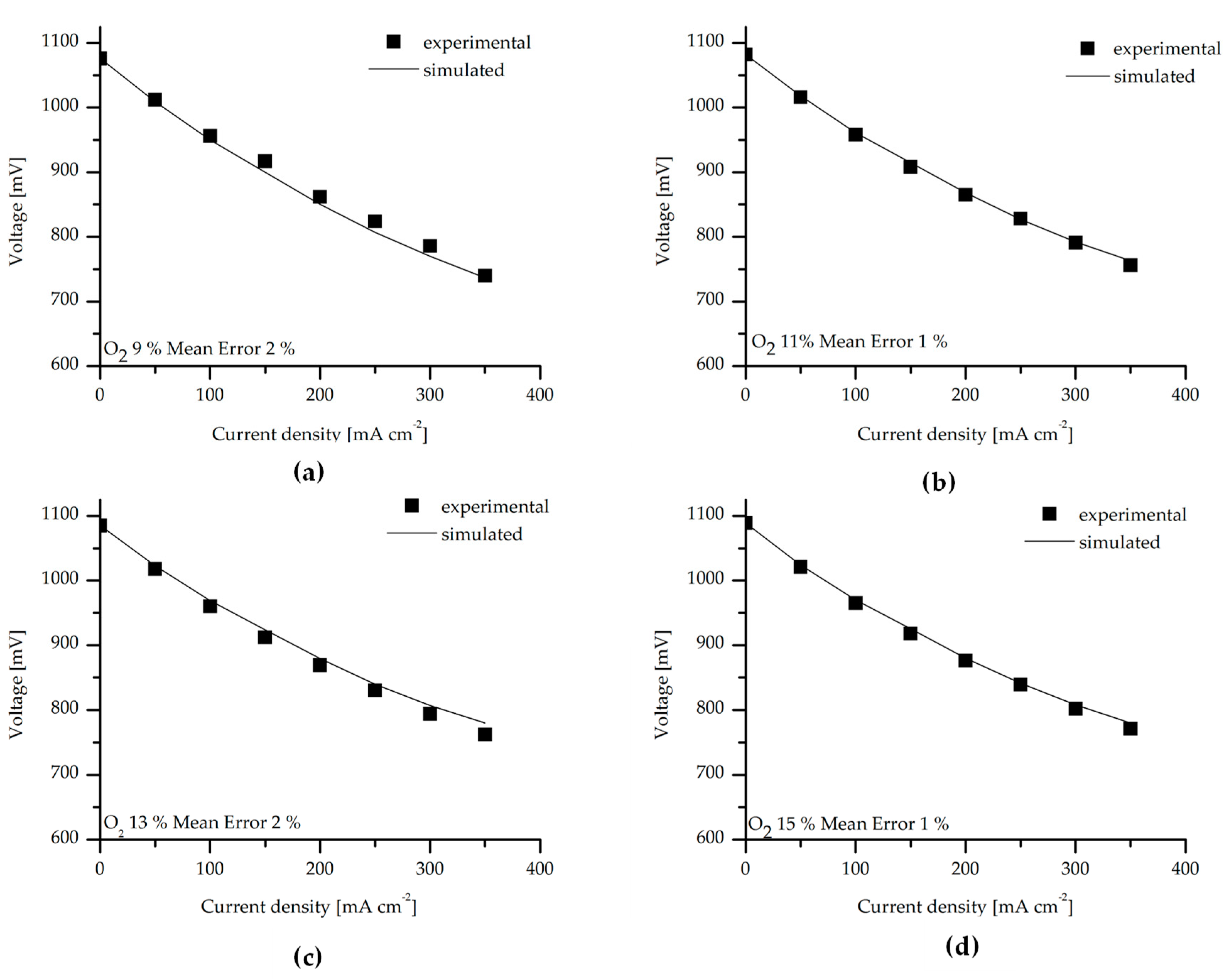
In Figure 4, Figure 5 and Figure 6, the obtained results concerning the comparison between experimental and calculated polarisation curves are reported. These figures refer to different operating conditions and, in each case, show a good agreement, with an average error of 1.7% on the voltages. The error does not show a particular trend and it is calculated in every graph as the average of the deviation between experimental and simulated data at the different current densities. In detail, Figure 4 and Figure 5 show how performance increases when the reactant concentration increases. A wider range of hydrogen concentrations has been tested to hypothesise different fuel types, while the oxygen concentration has been maintained around the typical value of industrial applications. In Figure 6, characteristic curves at different temperatures are reported and show the expected positive effect of the temperature increase on the performance due to the reduction of the resistances, despite the Nernst potential penalisation.

3.3. Local Validation

As above mentioned, by means of SIMFC it is possible to calculate the maps of the main chemical-physical variables on the cell plane, while the innovative test rig in the ENEA lab allows an evaluation of in-operando local values of temperature and hydrogen molar percentage at the anode side. In this way, simulated maps can be validated thanks to the available experimental local values.

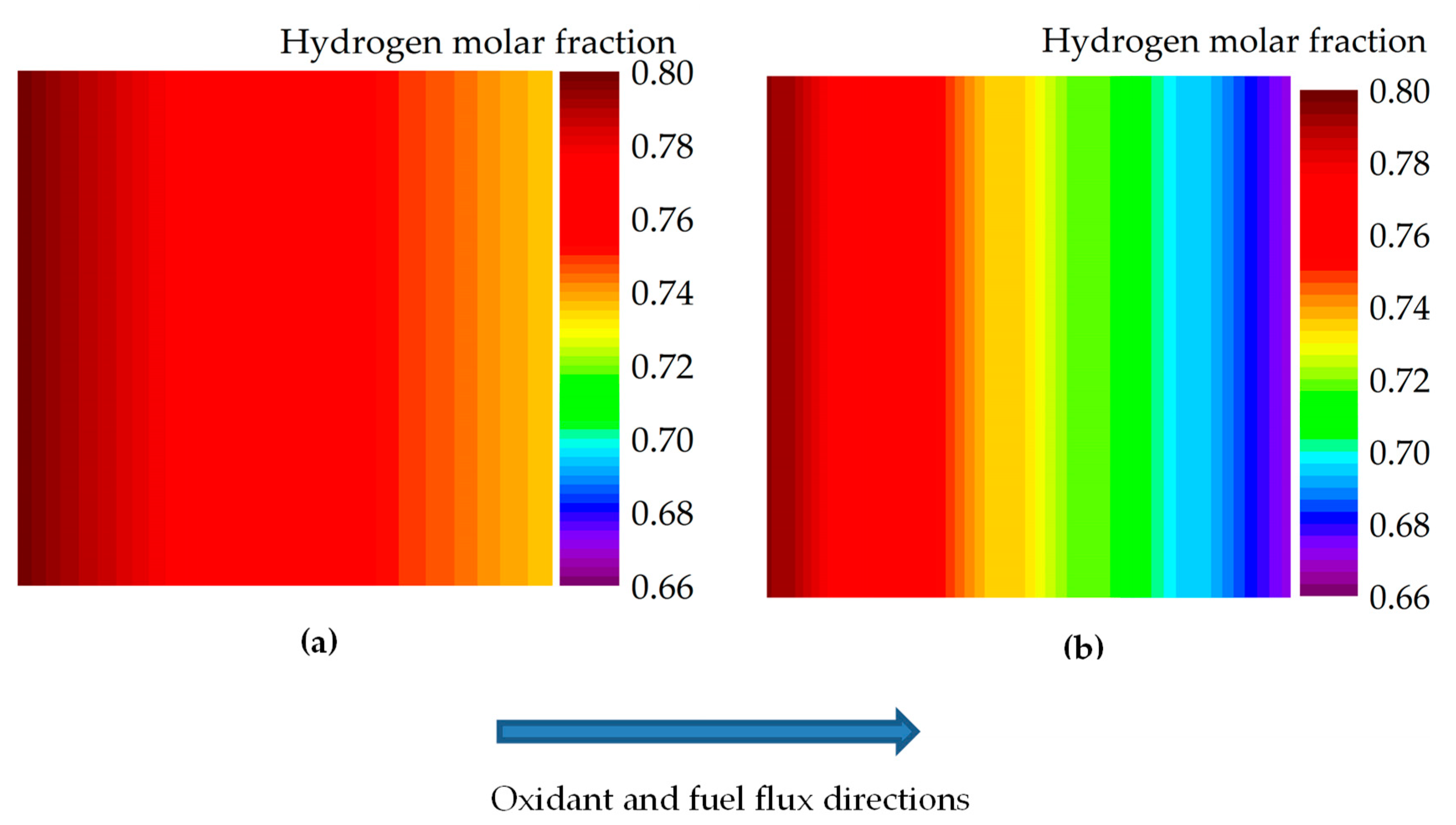
The results of the 2-D simulation are reported in Figure 7 in terms of hydrogen content and referring to the reference operating conditions at two electrical loads (123 mA cm⁻² and 248 mA cm⁻²).

As expected, from the inlet to the outlet in co-flow gas feeding configuration, the hydrogen content decreases due to the electrochemical reaction occurring in the fuel cell. The decrement is more evident at 248 mA cm⁻², where the fuel utilization factor is higher with respect to the electrical load condition at 123 mA cm⁻².

In Figure 8 there is a schematic representation of the position of the sampling points on the cell plane. The results of simulation are compared with the experimental values in

Table 5. Comparison of experimental and simulated local H₂ molar fraction (${\mathrm{x}}_{{\mathrm{H}}_2}$ ) under different loads on the cell plane.

Current Density	123 mA cm−2			248 mA cm−2
Sample point	Experimental (${\mathrm{x}}_{{\mathrm{H}}_2}$)	Simulated (${\mathrm{x}}_{{\mathrm{H}}_2}$)	Error (%)	Experimental (${\mathrm{x}}_{{\mathrm{H}}_2}$)	Simulated (${\mathrm{x}}_{{\mathrm{H}}_2}$)	Error (%)
1	0.8	0.78	2	0.79	0.77	2
2	0.80	0.78	2	0.78	0.77	1
3	0.80	0.78	2	0.78	0.77	1
4	0.76	0.78	2	0.79	0.76	4
5	0.78	0.77	1	0.78	0.74	5
6	0.77	0.76	1	0.78	0.72	8
7	0.78	0.75	3	0.77	0.72	6
8	0.76	0.75	1	0.77	0.7	9
9	0.68	0.74	9	0.68	0.69	1
10	0.69	0.74	7	0.67	0.69	3
11	0.69	0.74	7	0.66	0.69	4

.

The validation shows a satisfactory agreement between simulated and experimental results with an average error of 4%.

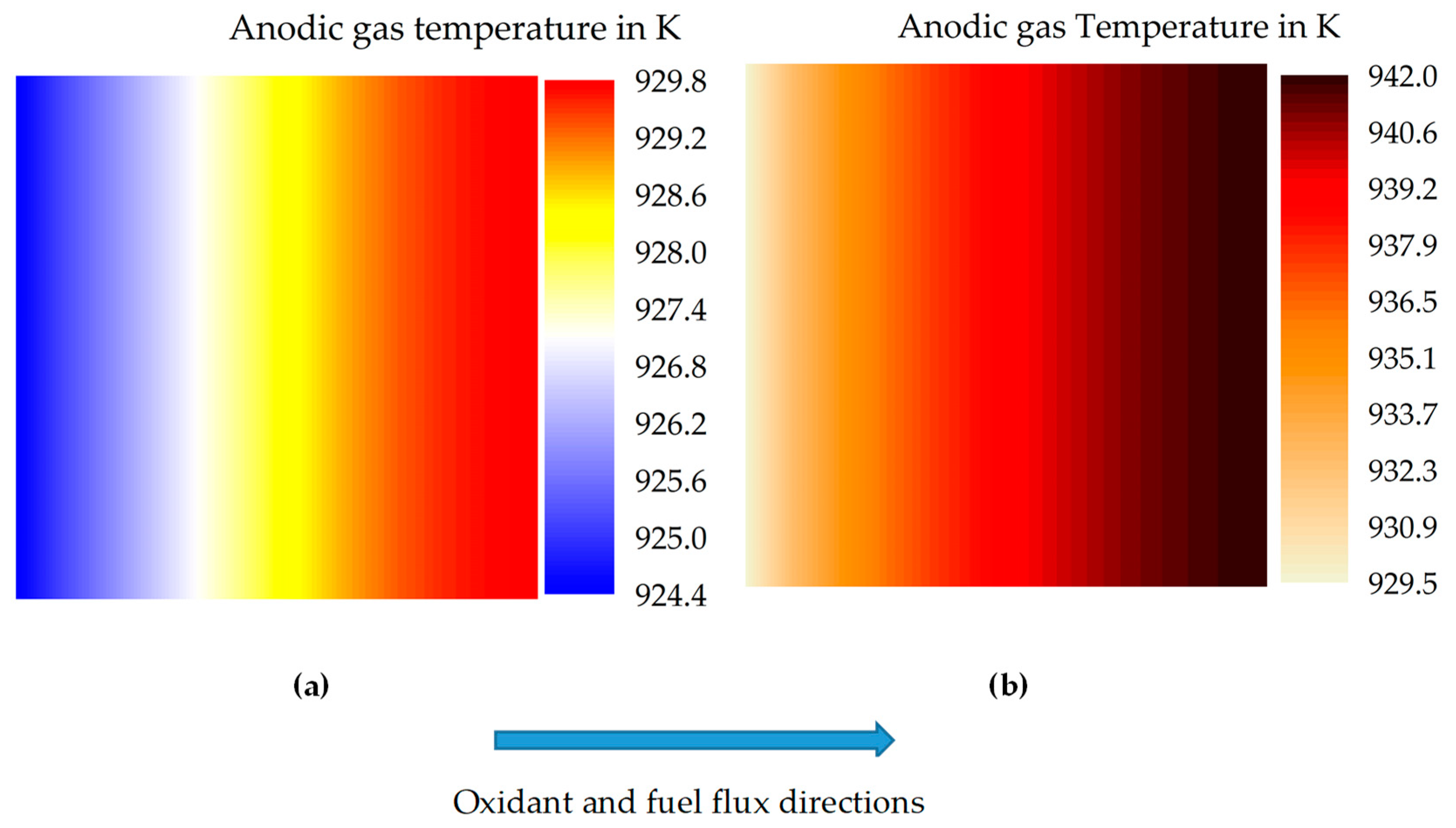
From a thermal point of view, Figure 9 shows the maps of the anodic gas temperature on the cell plane at the two studied current densities. Heat exchange through the top and bottom surfaces of the cell with the surrounding atmosphere of the test facility was predicted.

The temperature of the anodic gas, as expected, increases from the inlet to the outlet in both load conditions because of the co-flow feeding configuration of the test facility.

Similarly, in the case of the molar composition maps, in

Table 6. Comparison of experimental and simulated anodic gas temperature under different loads on the cell plane.

Current Density	123 mA cm−2			248 mA cm−2
Sample point	Experimental Temperature [K]	Simulated Temperature [K]	Error (%)	Experimental Temperature [K]	Simulated Temperature [K]	Error (%)
1	929.3	925.5	0.4	932.8	933.6	0.1
2	931.2	925.5	0.6	933	933.6	0.1
3	928.8	925.5	0.4	932.4	933.6	0.1
4	930.2	926.2	0.4	932.5	935.4	0.3
5	929.8	927	0.3	932.3	936.9	0.5
6	929.7	928.1	0.2	932.9	938.8	0.6
7	931.5	928.6	0.3	938.7	939.8	0.1
8	933.4	929.2	0.4	938.9	940.5	0.2
9	931.1	929.6	0.2	937.7	941.6	0.4
10	934.9	929.6	0.6	936.2	941.6	0.6
11	934.9	929.6	0.6	938.2	941.6	0.4

it is possible to compare simulated and experimental temperature values of the sampling points reported in Figure 8.

The agreement obtained is very good, with an average error of 0.3 % referring to all the available data.

4. Experimentation

The facility used for the experimentation is suitable for single cell operation and it was developed by ENEA in the framework of the “New all-European high-performance stack: Design for mass production (NELLHI)” European project. This test rig allows standard electrochemical tests such as polarization curves and EIS analysis, but the innovative feature is the possibility to measure the temperature and gas composition on the anode surface of the cell in real time using a gas chromatography and eleven thermocouples connected by means of eleven capillary tubes made out of AISI 310S stainless steel and welded perpendicularly in correspondence to the sampling ports. Some details of the unique and innovative test rig are shown in Figure 10. More exhaustive details of the experimental test rig can be found in [40,54]. As far as we know, another experimental test rig has been developed by Schiller et al. [55], but in that case, physical probes are used in a planar-segmented cell that also allows local measurements such as current density, voltage, temperature, and fuel concentrations along the flow path.

In the current work, anode supported IT-SOFC provided by Elcogen AS (Tallinn, Estony) has been tested.

The square planar single cells had a geometrical area of 144 cm² and an active area of 121 cm² and the main characteristics presented in

Table 7. Characteristics of the tested anode supported IT-SOFC.

Single Cell	Material	Thickness (µm)
Anode	Nickel- Yttra-Stabilzed Zirconia (Ni-YSZ)	350
Electrolyte	Yttra Stabilized Zirconia (YSZ)	5
Cathode	Lanthanum Strontium Cobaltite (LSC)	30

The electrodes porosity was 40% and 35% for anode and cathode respectively.

.

EIS has been measured in order to accurately evaluate the internal resistance of the cell. EIS measurements were carried out to analyse the frequency response of the cells tested, within the frequency range 10 kHz–0.01 Hz, using a frequency response analyser (FRA 1255B, Solartron Co., Farnborough, UK) coupled with an electrochemical dielectric interface (EI, 1287 Solartron Co., Farnborough, UK). All impedance measurements performed within this work were carried out under open-circuit conditions.

5. Conclusions

A new version of the SIMFC code has been set-up to allow the simulation of planar co-flow IT-SOFCs fed by H₂ as an ideal case study. The resulting 2-D code has been demonstrated to be a potential interesting tool, which can be useful for diagnostic and predictive issues.

The kinetic core of the model is a simplified semi-empirical formulation, which considers only the linear part of the polarization terms because of the low utilization factors used in the reference experimental tests.

Experiments on anode-supported single cells have been carried out feeding a humidified mixture of H₂ and N₂ at the anode and a mixture of O₂ and N₂ at the cathode and performing characteristic curves and EIS analyses at different operating conditions. The use of an innovative test facility with eleven sampling points allowed the detection of local temperature and hydrogen molar fraction on the anodic side.

The possibility of a model validation also on such local values represents a new outcome in this research area and can allow the set-up of a more reliable simulation tools to support the identification of a new technological solution or the optimisation of the operating conditions.

The preliminary comparison between experimental and calculated results showed a good agreement, with average errors equal to 1.4%, 4%, and 0.3% in terms of cell voltage, local H₂ molar fraction and local anodic gas temperature, respectively. The obtained results encourage further studies which allow the model validation on a greater quantity of data and under a wider range of operating conditions.

References

1. Emil, T.; Preis, H. Uber brennstoff-ketten mit festleitern. Ztschr. Elektrochem. 1937, 43, 727–732. [Google Scholar] [CrossRef]
2. Tarancón, A. Strategies for lowering solid oxide fuel cells operating temperature. Energies 2009, 2, 1130–1150. [Google Scholar] [CrossRef]
3. McPhail, S.J.; Conti, B.; Kiviaho, J. The Yellow Pages of SOFC Technology—International Status of SOFC deployment 2017; ENEA: Rome, Italy; VTT, Technical Research Centre of Finland Ltd.: Espoo, Finland, 2017; ISBN 978-88-8286-290-9. [Google Scholar]
4. Brett, D.J.L.; Atkinson, A.; Brandon, P.; Skinner, S.J.; Atkinson, A.; Brett, D.J.L. Intermediate temperature solid oxide fuel cells. Chem. Soc. Rev. 2008, 37, 1568–1578. [Google Scholar] [CrossRef] [PubMed]
5. Brandon, N.P.; Ruiz-Trejo, E.; Boldrin, P. Solid Oxide Fuel Cell Lifetime and Reliability, 1st ed.; Academic Press: London, UK, 2017; ISBN 9780081011027. [Google Scholar]
6. D’Andrea, G.; Gandiglio, M.; Lanzini, A.; Santarelli, M. Dynamic model with experimental validation of a biogas-fed SOFC plant. Energy Convers. Manag. 2017, 135, 21–34. [Google Scholar] [CrossRef]
7. Brunaccini, G.; Sergi, F.; Aloisio, D.; Ferraro, M.; Blesznowski, M.; Kupecki, J.; Motylinski, K.; Antonucci, V. Modeling of a SOFC-HT battery hybrid system for optimal design of off-grid base transceiver station. Int. J. Hydrogen Energy 2017, 42, 27962–27978. [Google Scholar] [CrossRef]
8. Safari, A.; Shahsavari, H.; Salehi, J. A mathematical model of SOFC power plant for dynamic simulation of multi-machine power systems. Energy 2018, 149, 397–413. [Google Scholar] [CrossRef]
9. Kupecki, J.; Motylinski, K.; Milewski, J. Dynamic analysis of direct internal reforming in a SOFC stack with electrolyte-supported cells using a quasi-1D model. Appl. Energy 2017, 227, 1–8. [Google Scholar] [CrossRef]
10. Cheddie, D.F. Integration of a solid oxide fuel cell into a 10 MW gas turbine power plant. Energies 2010, 3, 754–769. [Google Scholar] [CrossRef]
11. Rabbani, A.; Rokni, M. Modeling and analysis of transport processes and efficiency of combined SOFC and PEMFC systems. Energies 2014, 7, 5502–5522. [Google Scholar] [CrossRef]
12. Tang, S.; Amiri, A.; Vijay, P.; Tadé, M.O. Development and validation of a computationally efficient pseudo 3D model for planar SOFC integrated with a heating furnace. Chem. Eng. J. 2016, 290. [Google Scholar] [CrossRef]
13. Ghorbani, B.; Vijayaraghavan, K. 3D and simplified pseudo-2D modeling of single cell of a high temperature solid oxide fuel cell to be used for online control strategies. Int. J. Hydrogen Energy 2018, 43, 9733–9748. [Google Scholar] [CrossRef]
14. Amiri, A.; Vijay, P.; Tadé, M.O.; Ahmed, K.; Ingram, G.D.; Pareek, V.; Utikar, R. Planar SOFC system modelling and simulation including a 3D stack module. Int. J. Hydrogen Energy 2016, 41, 2919–2930. [Google Scholar] [CrossRef] [Green Version]
15. Zhang, Z.; Chen, J.; Yue, D.; Yang, G.; Ye, S.; He, C.; Wang, W.; Yuan, J.; Huang, N. Three-dimensional CFD modeling of transport phenomena in a cross-flow anode-supported planar SOFC. Energies 2014, 7, 80–98. [Google Scholar] [CrossRef]
16. Shen, S.; Kuang, Y.; Zheng, K.; Gao, Q. A 2D model for solid oxide fuel cell with a mixed ionic and electronic conducting electrolyte. Solid State Ionics 2018, 315, 44–51. [Google Scholar] [CrossRef]
17. Luo, X.J.; Fong, K.F. Development of 2D dynamic model for hydrogen-fed and methane-fed solid oxide fuel cells. J. Power Sources 2016, 328, 91–104. [Google Scholar] [CrossRef]
18. Aydın, Ö.; Nakajima, H.; Kitahara, T. Reliability of the numerical SOFC models for estimating the spatial current and temperature variations. Int. J. Hydrogen Energy 2016, 41, 15311–15324. [Google Scholar] [CrossRef]
19. Costamagna, P.; Grosso, S.; Travis, R.; Magistri, L. Integrated planar solid oxide fuel cell: Steady-state model of a bundle and validation through single tube experimental data. Energies 2015, 8, 13231–13254. [Google Scholar] [CrossRef]
20. Yuan, K.; Ji, Y.; Chung, J.N. Physics-based modeling of a low-temperature solid oxide fuel cell with consideration of microstructure and interfacial effects. J. Power Sources 2009, 194, 908–919. [Google Scholar] [CrossRef]
21. Pramuanjaroenkij, A.; Kakaç, S.; Yang Zhou, X. Mathematical analysis of planar solid oxide fuel cells. Int. J. Hydrog. Energy 2008, 33, 2547–2565. [Google Scholar] [CrossRef]
22. Jeon, D.H. A comprehensive CFD model of anode-supported solid oxide fuel cells. Electrochim. Acta 2009, 54, 2727–2736. [Google Scholar] [CrossRef]
23. Iora, P.; Aguiar, P.; Adjiman, C.S.; Brandon, N.P. Comparison of two IT DIR-SOFC models: Impact of variable thermodynamic, physical, and flow properties. Steady-state and dynamic analysis. Chem. Eng. Sci. 2005, 60, 2963–2975. [Google Scholar] [CrossRef]
24. Cheddie, D.F.; Munroe, N.D.H. A dynamic 1D model of a solid oxide fuel cell for real time simulation. J. Power Sources 2007, 171, 634–643. [Google Scholar] [CrossRef]
25. Kang, Y.; Li, J.; Cao, G.; Tu, H.; Li, J.; Yang, J. One-dimensional dynamic modeling and simulation of a planar direct internal reforming solid oxide fuel cell. Chin. J. Chem. Eng. 2009, 17, 304–317. [Google Scholar] [CrossRef]
26. Wang, C.; Nehrir, M.H. A physically based dynamic model for solid oxide fuel cells. IEEE Trans. Energy Convers. 2007, 22, 887–897. [Google Scholar] [CrossRef]
27. Wang, C.; Nehrir, M.H.; Shaw, S.R. Dynamic models and model validation for PEM fuel cells using electrical circuits. IEEE Trans. Energy Convers. 2005, 20, 442–451. [Google Scholar] [CrossRef]
28. Chan, S.; Khor, K.; Xia, Z. A complete polarization model of a solid oxide fuel cell and its sensitivity to the change of cell component thickness. J. Power Sources 2001, 93, 130–140. [Google Scholar] [CrossRef]
29. Sorrentino, M.; Pianese, C. Grey-Box modeling of SOFC unit for design, control and diagnostics applications grey-box modeling of SOFC unit for design, control and diagnostics applications. In Proceedings of the European Fuel Cell Forum, Lucerne, Switzerland, 29 July 2009. [Google Scholar]
30. Sorrentino, M.; Pianese, C.; Guezennec, Y.G. A hierarchical modeling approach to the simulation and control of planar solid oxide fuel cells. J. Power Sources 2008, 180, 380–392. [Google Scholar] [CrossRef]
31. Razbani, O.; Assadi, M. Artificial neural network model of a short stack solid oxide fuel cell based on experimental data. J. Power Sources 2014, 246, 581–586. [Google Scholar] [CrossRef]
32. Bicer, Y.; Dincer, I.; Aydin, M. Maximizing performance of fuel cell using artificial neural network approach for smart grid applications. Energy 2016, 116, 1205–1217. [Google Scholar] [CrossRef]
33. Polverino, P.; Sorrentino, M.; Pianese, C. Improved Fault Isolability for solid oxide fuel cell diagnosis through Sub-system analysis. Energy Procedia 2017, 105, 1918–1923. [Google Scholar] [CrossRef]
34. Koeppel, B.J.; Lai, C.; Iyengar, A.K.S.; Xu, Z.; Wang, C.; Hackett, G.A. Use of a Reduced Order Model (ROM) to simulate SOFC performance in system models. ECS Trans. 2017, 78, 2595–2605. [Google Scholar] [CrossRef]
35. Chakraborty, U.K.; Abbott, T.E.; Das, S.K. PEM fuel cell modeling using differential evolution. Energy 2012, 40, 387–399. [Google Scholar] [CrossRef]
36. Chakraborty, U.K. Static and dynamic modeling of solid oxide fuel cell using genetic programming. Energy 2009, 34, 740–751. [Google Scholar] [CrossRef]
37. Bosio, B.; Di Giulio, N.; Nam, S.W.; Moreno, A. An effective semi-empiric model for MCFC kinetics: Theoretical development and experimental parameters identification. Int. J. Hydrog. Energy 2014, 39, 12273–12284. [Google Scholar] [CrossRef]
38. Arato, E.; Audasso, E.; Barelli, L.; Bosio, B.; Discepoli, G. Kinetic modelling of molten carbonate fuel cells: Effects of cathode water and electrode materials. J. Power Sources 2016, 330, 18–27. [Google Scholar] [CrossRef]
39. Audasso, E.; Barelli, L.; Bidini, G.; Bosio, B.; Discepoli, G. Molten carbonate fuel cell performance analysis varying cathode operating conditions for carbon capture applications. J. Power Sources 2017, 348, 118–129. [Google Scholar] [CrossRef]
40. Santoni, F.; Silva Mosqueda, D.M.; Pumiglia, D.; Viceconti, E.; Conti, B.; Boigues Muñoz, C.; Bosio, B.; Ulgiati, S.; McPhail, S.J. In-situ study of the gas-phase composition and temperature of an intermediate-temperature solid oxide fuel cell anode surface fed by reformate natural gas. J. Power Sources 2017, 370, 36–44. [Google Scholar] [CrossRef]
41. Fuel Cell Handbook, 7th ed.; EG&G Technical Services, Inc.: Morgantown, WV, USA, 2004; ISBN 0442319266.
42. Leonide, A.; Apel, Y.; Ivers-Tiffée, E. SOFC modeling and parameter identification by means of impedance spectroscopy. ECS Trans. 2009, 19, 81–109. [Google Scholar] [CrossRef]
43. Boigues-Muñoz, C.; Pumiglia, D.; McPhail, S.J.; Santori, G.; Montinaro, D.; Comodi, G.; Carlini, M.; Polonara, F. More accurate macro-models of solid oxide fuel cells through electrochemical and microstructural parameter estimation—Part II: Parameter estimation. J. Power Sources 2015, 286, 321–329. [Google Scholar] [CrossRef]
44. Costamagna, P.; Selimovic, A.; Del Borghi, M.; Agnew, G. Electrochemical model of the integrated planar solid oxide fuel cell (IP-SOFC). Chem. Eng. J. 2004, 102, 61–69. [Google Scholar] [CrossRef]
45. Ni, M.; Leung, M.K.H.; Leung, D.Y.C. Parametric study of solid oxide fuel cell performance. Energy Convers. Manag. 2007, 48, 1525–1535. [Google Scholar] [CrossRef]
46. Mizusaki, J.; Tagawa, H.; Saito, T.; Yamamura, T.; Kamitani, K.; Hirano, K.; Ehara, S.; Takagi, T.; Hikita, T.; Ippommatsu, M.; et al. Kinetic studies of the reaction at the nickel pattern electrode on YSZ in H2H2O atmospheres. Solid State Ionics 1994, 70–71, 52–58. [Google Scholar] [CrossRef]
47. Marra, D.; Bosio, B. Process analysis of 1 MW MCFC plant. Int. J. Hydrogen Energy 2007, 32, 809–818. [Google Scholar] [CrossRef]
48. Bosio, B.; Marra, D.; Arato, E. Thermal management of the molten carbonate fuel cell plane. J. Power Sources 2010, 195, 4826–4834. [Google Scholar] [CrossRef]
49. Chakraborty, U.K. Reversible and irreversible potentials and an inaccuracy in popularmodels in the fuel cell literature. Energies 2018, 11, 1851. [Google Scholar] [CrossRef]
50. Greene, E.S.; Chiu, W.K.S.; Burke, A.A.; Medeiros, M.G.; Carreiro, L.G. Modeling and verification of steady state operational changes on the performance of a solid oxide fuel cell. J. Fuel Cell Sci. Technol. 2009, 6, 041001. [Google Scholar] [CrossRef]
51. Achenbach, E. Three-dimensional and time-dependent simulation of a planar solid oxide fuel cell stack. J. Power Sources 1994, 49, 333–348. [Google Scholar] [CrossRef]
52. Yahya, A.; Ferrero, D.; Dhahri, H.; Leone, P.; Slimi, K.; Santarelli, M. Electrochemical performance of solid oxide fuel cell: Experimental study and calibrated model. Energy 2018, 142, 932–943. [Google Scholar] [CrossRef]
53. Nagata, S.; Momma, A.; Kato, T.; Kasuga, Y. Numerical analysis of output characteristics of tubular SOFC with internal reformer. J. Power Sources 2001, 101, 60–71. [Google Scholar] [CrossRef]
54. Pumiglia, D.; Santoni, F.; Viceconti, E.; Conti, B.; Boigues Muñoz, C.; Bosio, B.; Carlini, M.; McPhail, S.J. SOFC anode process characterization by means of a spot-sampling set-up for in-operando gas analysis. ECS Trans. 2016, 75, 1–8. [Google Scholar] [CrossRef]
55. Bessler, W.G.; Gewies, S.; Willich, C.; Schiller, G.; Friedrich, K.A. Spatial distribution of electrochemical performance in a segmented SOFC: A combined modeling and experimental study. Fuel Cells 2010, 10, 411–418. [Google Scholar] [CrossRef]
Figure 1. (a) Characteristic curves and (b) EIS at reference temperature (923 K) and cathodic composition (21% O2), varying the anodic composition.
Catalysts 09 00036 g001
Figure 2. (a) Characteristic curves and (b) EIS at reference temperature (923 K) and anodic composition (80% H2), varying the cathodic composition.
Catalysts 09 00036 g002
Figure 3. (a) Characteristic curves and (b) EIS at reference composition (80% H2, 21% O2) and varying the operating temperature.
Catalysts 09 00036 g003
Figure 4. Simulation of the characteristics curves using SIMFC: different anodic compositions (a) H2 96%, (b) H2 80%, (c) H2 60%, and (d) H2 40%, with cathodic composition 21% O2.
Catalysts 09 00036 g004
Figure 5. Simulation of the characteristics curves using SIMFC: different cathodic compositions (a) O2 9%, (b) O2 11%, (c) O2 13%, (d) O2 15%, with anodic composition 80% H2.
Catalysts 09 00036 g005
Figure 6. Simulation of the characteristic curves using SIMFC: different temperatures (a) T 948, (b) T 973, and (c) T 998 with anodic composition 80% H2 and cathodic composition 21 % O2.
Catalysts 09 00036 g006
Figure 7. Simulated maps of hydrogen molar fraction for the reference conditions (21% O2, 80% H2, 923 K) at (a) 123 mA cm−2 and (b) 248 mA cm−2.
Catalysts 09 00036 g007
Figure 8. Position of the sampling points on the cell plane.
Catalysts 09 00036 g008
Figure 9. Simulated maps of the anodic gas temperature for the reference conditions at (a) 123 mA cm−2 and (b) 248 mA cm−2.
Catalysts 09 00036 g009
Figure 10. Section of the experimental setup.
Catalysts 09 00036 g010