Surface Anchoring Effects on the Formation of Two-Wavelength Surface Patterns in Chiral Liquid Crystals


Department of Chemical Engineering, McGill University, 3610 University Street, Montreal, QC H3A 2B2, Canada
*
Author to whom correspondence should be addressed.
Crystals 2019, 9(4), 190; https://doi.org/10.3390/cryst9040190
Submission received: 26 February 2019
/
Revised: 25 March 2019
/
Accepted: 26 March 2019
/
Published: 2 April 2019
(This article belongs to the Special Issue Advances in Cholesteric Liquid Crystals)
Abstract
:We present a theoretical analysis and linear scaling of two-wavelength surface nanostructures formed at the free surface of cholesteric liquid crystals (CLC). An anchoring model based on the capillary shape equation with the high order interaction of anisotropic interfacial tension is derived to elucidate the formation of the surface wrinkling. We showed that the main pattern-formation mechanism is originated due to the interaction between lower and higher order anchoring modes. A general phase diagram of the surface morphologies is presented in a parametric space of anchoring coefficients, and a set of anchoring modes and critical lines are defined to categorize the different types of surface patterns. To analyze the origin of surface reliefs, the correlation between surface energy and surface nano-wrinkles is investigated, and the symmetry and similarity between the energy and surface profile are identified. It is found that the surface wrinkling is driven by the director pressure and is annihilated by two induced capillary pressures. Linear approximation for the cases with sufficient small values of anchoring coefficients is used to realize the intrinsic properties and relations between the surface curvature and the capillary pressures. The contributions of capillary pressures on surface nano-wrinkling and the relations between the capillary vectors are also systematically investigated. These new findings establish a new approach for characterizing two-length scale surface wrinkling in CLCs, and can inspire the design of novel functional surface structures with the potential optical, friction, and thermal applications.
1. Introduction
A variety of periodic surface structures and wrinkled textures are widely found in the plant and animal kingdoms [1,2,3,4,5,6]. Since these surface ultrastructures with micro/nano scale features provide unique optical responses and iridescent colors [7,8,9,10,11], understanding their formation mechanism is crucial in realizing structural color in nature and in biomimetic design of novel photonic systems. As similar nano/micro scale periodic wrinkles are formed at the free surface of both synthetic and biological cholesteric liquid crystals (CLCs) [12,13], and CLC phases are widely found in Nature and living soft materials both in vivo and vitro [13,14], nematic liquid crystal self-assembly has been proposed as the formation mechanism of helicoidal plywoods and the surface ultrastructures in many fibrous composites ranging from plant cell walls to arthropod cuticles [15,16,17,18,19]. Moreover, it has been shown that the characteristics of chiral phases control the unique colors and optical properties exhibited in the films and fibers made by cellulose-based CLCs [20,21].
Inspired by surface ultrastructure in Nature, engineered surface structures incorporating chiral nematic structures can be fabricated to mimic the unique optical properties. If the formation of the surface patterns can be efficiently captured by a rigorous model based on a CLC mesophase, we can elucidate the pattern formation mechanisms for the construction of biomimetic proof-of-concept prototypes. In our previous works [22,23,24], significant efforts have been made in formulating and validating theoretical models to explain the formation of surface wrinkles in a plant-based CLC as a model material system. We identified the chiral capillary pressure, known as director pressure, that reflects the anisotropic nature of CLC through the orientation contribution to the surface energy as the fundamental driving force in generating single-wavelength wrinkling. However, surface wrinkling in nature can include more complex patterns such as multiple-length-scale undulations [11,25,26,27]. To elucidate this feature, we previously proposed a physical model [28,29] that combines membrane bending elasticity and liquid crystal anchoring. A rich variety of multi-scale complex patterns, such as spatial period-doubling and period-tripling are presented for the cases in which the anchoring and bending effects are comparable [28]. In a recent communication [30], we briefly presented a pure higher order anchoring model in the absence of bending elasticity, surprisingly capturing multiple length-scale surface wrinkles. In this previous work, a novel mechanism for the formation of two-scale nano-wrinkling was proposed, which was exclusively based on anchoring energy including quartic harmonics. Here, we present a complete and rigorous new analysis of the multiple-length-scale surface wrinkles based on the pure higher order anchoring model in full detail and approximate the response of the surface structure to chirality and anchoring coefficients based on a linear model. In addition, a fundamental characterization of the capillary vector and capillary pressures required to connect surface geometry and mechanical forces is presented.
The objective of this paper is to identify the key mechanisms that induce and resist the multiple-length-scale surface wrinkling in CLCs based on a pure higher order anchoring model. To develop the anchoring model, we used the generalized shape equation for anisotropic interfaces using the Cahn-Hoffman capillarity [31] and the Rapini-Papoular quartic anchoring energy [32]. The presented model depicts the formation mechanism of two-length scale surface patterns based on the interaction between lower and higher order anchoring modes. The linear approximations of surface curvatures are derived to provide the explicit relations between the anchoring coefficients, helix pitch, and surface profile of the two-length scale wrinkles. These new findings can establish a new strategy for characterizing two-length scale surface wrinkling in biological CLCs, and inspire the design of novel functional surface structures with the potential optical, friction, and thermal applications.
The organization of this paper is as follows. Section 2 presents the geometry and structure of the CLC system. Section 3 presents the governing nemato-capillary shape equation expressing the coupling mechanism between the surface geometry and anisotropic ordering for a CLC free interfaces with a quartic anchoring energy and a pure surface splay-bend deformation. Appendix A presents the details of the derivation of the Cahn-Hoffman capillary vector thermo-dynamics for CLC interfaces. Appendix B describes the capillary shape equation in terms of three capillary pressures. Appendix C represents the shape equation based on the driving and resisting terms. Section 4 analyzes the effect of anchoring coefficients and helix pitch on the surface normal angle and the resultant surface profile. In this section, a general phase diagram of surface profiles in the parametric of anchoring coefficients is presented and the origin of the two scales is revealed through the linear theory. Then, the linear approximations of surface curvatures, assuming small values of anchoring coefficients, are derived to identify the leading mechanism controlling the surface wrinkling. Appendix D proposes the analytical expression for the linear approximation of the surface relief. The surface energy associated with the CLC interface is also analyzed to establish an energy transfer mechanism from anchoring energy of a flat surface into a wrinkled surface. Furthermore, the surface wrinkles are evaluated through analyzing the three capillary pressures, and the pressure–curvature relations are introduced to explore the variation of curvature profile with respect to the capillary pressures. Appendix E represents the derivation of the pressure–curvature relations. Finally, the capillary vectors are formulated to provide a clear physical explanation for the formation of the surface wrinkles. Appendix F formulates the capillary vectors. Section 5 presents the conclusions.
2. Geometry and Structure
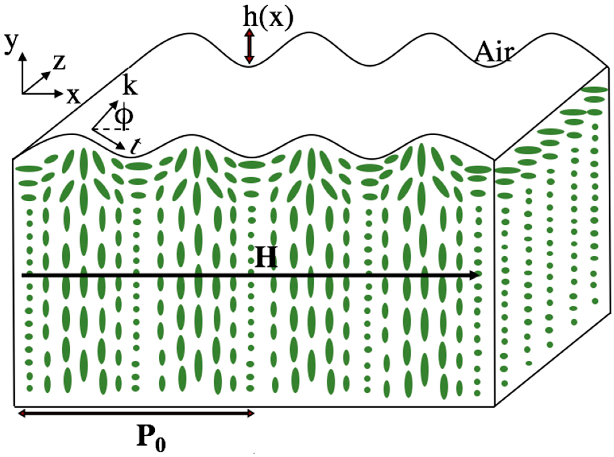
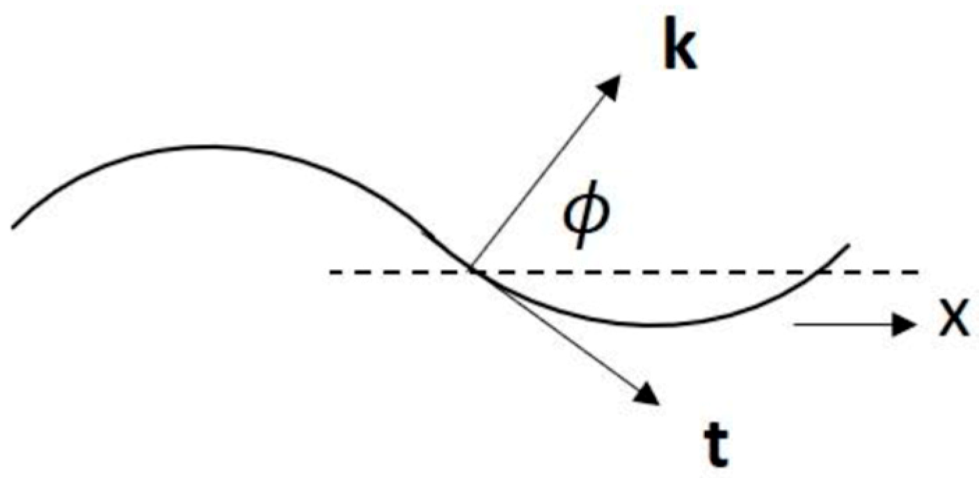
Figure 1 depicts the schematics of the CLC structure where ellipsoids indicate fiber orientation on each parallel layer. We assume that the helix axis, H is parallel to the surface; other complex structures occurring when the helix axis H is distorted are beyond the scope of this paper. The fiber orientation at the interface is defined by the director n. The pitch length P0 is defined as the distance through which the fibers undergo a 2π rotation. For a rectangular (x,y,z) coordinate system, the surface relief that is directed along the x axis can be described by a y(x,z) deviation from the xz plane. The amplitude of the vertical undulation is h(x). As the surface relief is constant in the z direction for a linear texture, the curvature in the z-direction is zero. The unit tangent, t, and the unit normal, k, to the surface can be expressed with the normal angle, φ: , . L is the given system length in the x direction. The arc-length measure of the undulating surface is “s”.
3. Governing Equations
In this paper, we assume that the multi-length scale surface wrinkles are formed through modulation in surface energy at the anisotropic-air interface of CLCs. The typical capillary shape equations, which are generalized forms of a Laplace equation including the liquid crystal order and gradient density have been comprehensively formulated and previously presented for liquid crystal fibers, membranes, films, and drops [33]. Here, the coupling mechanism between the surface geometry and CLC order are demonstrated through the capillarity shape equation for CLC free interfaces with a pure surface splay-bend deformation.
The formation of surface nanostructures in CLC interfaces is a complex phenomenon involving interfacial tension, surface anchoring energy, and bulk Frank elasticity that requires integrated multi-scale modelling of bulk and surface. However, the analytic solution of the problem with the usual formalism is very complicated. Here, we assume a cholesteric director field in the bulk region, , and a splay-bend director field at the interface where , is the director angle, q is the wave vector, and P0 is the helix pitch.
Based on the generalized Rapini-Papoular equation [24], the interfacial surface energy, between a liquid crystal phase and another phase can be described by [32]
where is the isotropic contribution, n is the director field at the interface, k is the surface unit normal, and are the temperature/concentration dependent anchoring coefficients. The preferred orientation that minimizes the anchoring energy (Equation (1)) is known as the easy axis. The actual stationary surface director orientation is the result of a balance between surface anchoring and bulk gradient Frank elasticity [34]. For the cases in which the gradient Frank elasticity is insignificant, the actual stationary and preferred director fields are identical. As shown in ref. [22], for the cholesteric–air interface with quite strong anchoring, the gradient Frank elasticity is negligible in comparison with anchoring in the formation of the surface undulations. It should be noted that here we neglect the Marangoni flow that is likely to be formed due to the orientational-driven surface tension gradients [35,36,37]. Other effects and processes such as 3D orientation structures, strong nonlinearities, hydrodynamic [38,39], and viscoelastic effects [40,41,42] discussed elsewhere are beyond the scope of this paper.
The generalized Cahn-Hoffman capillary vector [43,44], is the fundamental quantity that reflects the anisotropic contribution of CLC in the capillary shape equation. It contains two orthogonal components: normal vector, representing the increase in surface energy through dilation (change in area) and tangent vector, representing the change in surface energy through rotation of the unit normal. The derivation details of the Cahn-Hoffman capillary vector thermodynamics for anisotropic interfaces are given in Appendix A [31].
Here is the unit surface dyadic, and is the identity tensor. The dyadic is similar to due to , where t is the unit tangent and R is the rotation matrix satisfying (see refs [45] and [46] for details):
The following identity holds:
The interfacial static force balance equation at the CLC/air interface is expressed by
where represent the total stress tensor in the air and the bulk CLC phase, is the surface gradient operator, and is the interface stress tensor. The air and the bulk CLC stress tensor, are given by
where are the hydrostatic pressures, is the bulk Frank energy density, and is the Ericksen stress tensor. The bulk Frank energy density for a CLC reads
where are splay, twist, and blend elastic constant, respectively. is saddle-splay elastic constant. The Ericksen stress tensor, is given by
The projection of Equation (6) along direction k yields the capillary shape equation:
where stress jump, SJ, is the total normal stress jump, and is the capillary pressure. Usually we take , and consider the other terms as elastic correction. The interfacial torque balance equation is given by
where is the Lagrange multiplier and h is the surface molecular field composed by two parts:
Here is the gradient interfacial free-energy density defined by introducing surface gradient energy density vector g:
By multiplying on both sides of Equation (11), the torque balance equation can be rewritten in a compact form:
Equation (14) gives an alternative path to compute . The expansion of the term reads
which gives . Thus, only the bulk energy density, , contributes to the elastic correction, which is negligible [22]. For typical cholesteric liquid crystals, the internal length K/γ0 is in the range 1 nm (an order of magnitude estimation of the elastic constant K and the surface tension γ0 gives K ≈ 10−11 J/m and γ0 ≈ 10−2 J/m2) [43]. As the ratio of W/γ0 at the cholesteric–air interface with quite strong anchoring lies in the range (B = W/γ0 = 0.01), the extrapolation length scale K/W is about . With these values, for a typical CLC with a pitch , the ratio of extrapolation length scale to pitch is in the order of So, the elastic correction contributes 8% to the shape equation, and can be neglected to describe nano-scale surface undulations. As the result, the final shape equation becomes (see Appendix B)
The first two terms contain , providing information about the surface curvature where is the normal angle and is the arc-length. The first term on the right-hand side of Equation (16), which is the usual Laplace pressure, corresponds to the contribution from the normal component of the Cahn-Hoffman capillary vector. The second term which is the anisotropic pressure due to preferred orientation (known as Herring’s pressure) corresponds to the contribution from the tangential component of the Cahn-Hoffman capillary vector . The last term in Equation (16) represents the additional contribution to the capillary pressure which corresponds to the director curvature due to orientation gradients (see Appendix C). Considering a rectangular coordinate system (x,y,z), where x is the wrinkling direction, and y is the vertical axis, and considering the typical quartic anchoring model [24], , yields the nonlinear ordinary differential equation (ODE) in terms of normal angle, :
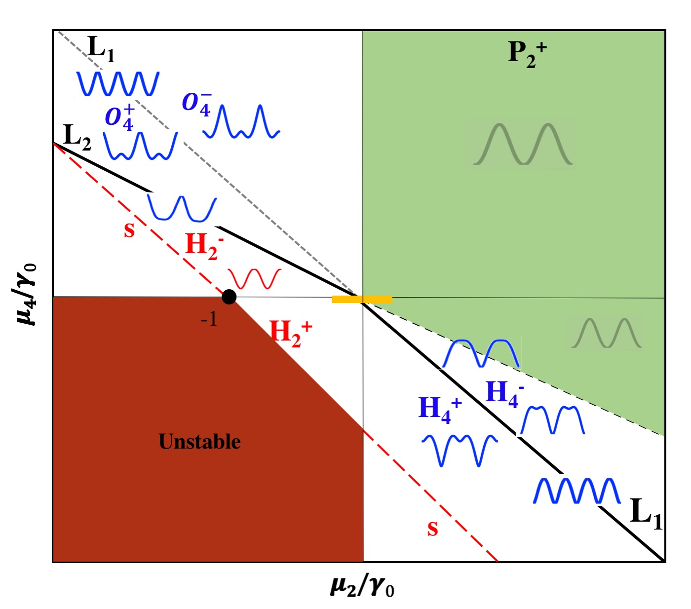
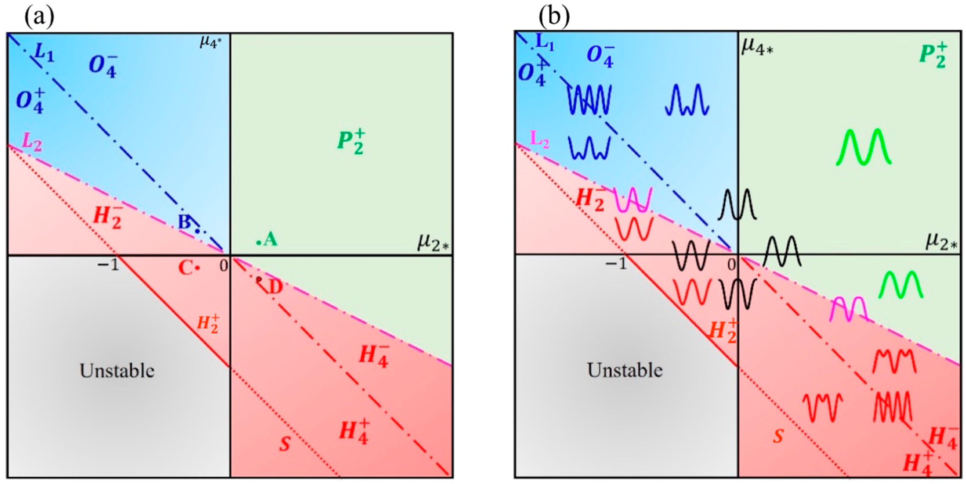
Here denotes as the driving force and the resistant term. The boundary condition at x = 0 is ; and are the scaled anchoring coefficients divided by isotropic surface tension , and ; and is the approximation of . The generic features of the normal angle and its periodicity are the important outputs of the shape equation. There are three significant system parameters that have influence on the : the scaled anchoring coefficients , and the sign and magnitude of the helix pitch P0. Thus, the surface profile is a function of two material properties and one structural order parameter (P0). In the following context, we always assume that helix pitch is constant at P0 = 1.2 μm. Figure 2a depicts the regions with different surface wrinkling in the parametric space of the scaled anchoring coefficients: . Here O, H, and P refer to oblique, homeotropic, and planar director anchoring modes, respectively. The reader is directed to reference [30] for a full discussion of these fundamental states. The subscript numbers in O, H, and P indicate the wave number of morphologies in one period, and the superscript sign differentiates the anchoring modes. The transition lines and are defined as and , and the thermodynamic stability line (γ = 0) is . Points A, B, C, and D are chosen as the representative points in , , , and regions with : A(0.002, 0.001), B(−0.002, 0.0015), C(−0.002, −0.001), and D(0.002, −0.0015). Points A and C, and B and D are related by rotation symmetry. It should be noted that for the cases in which the quartic anchoring is zero, only single-wavelength sinusoidal profile can be obtained in the linear regime ().
4. Results and Discussion
4.1. Surface Profile
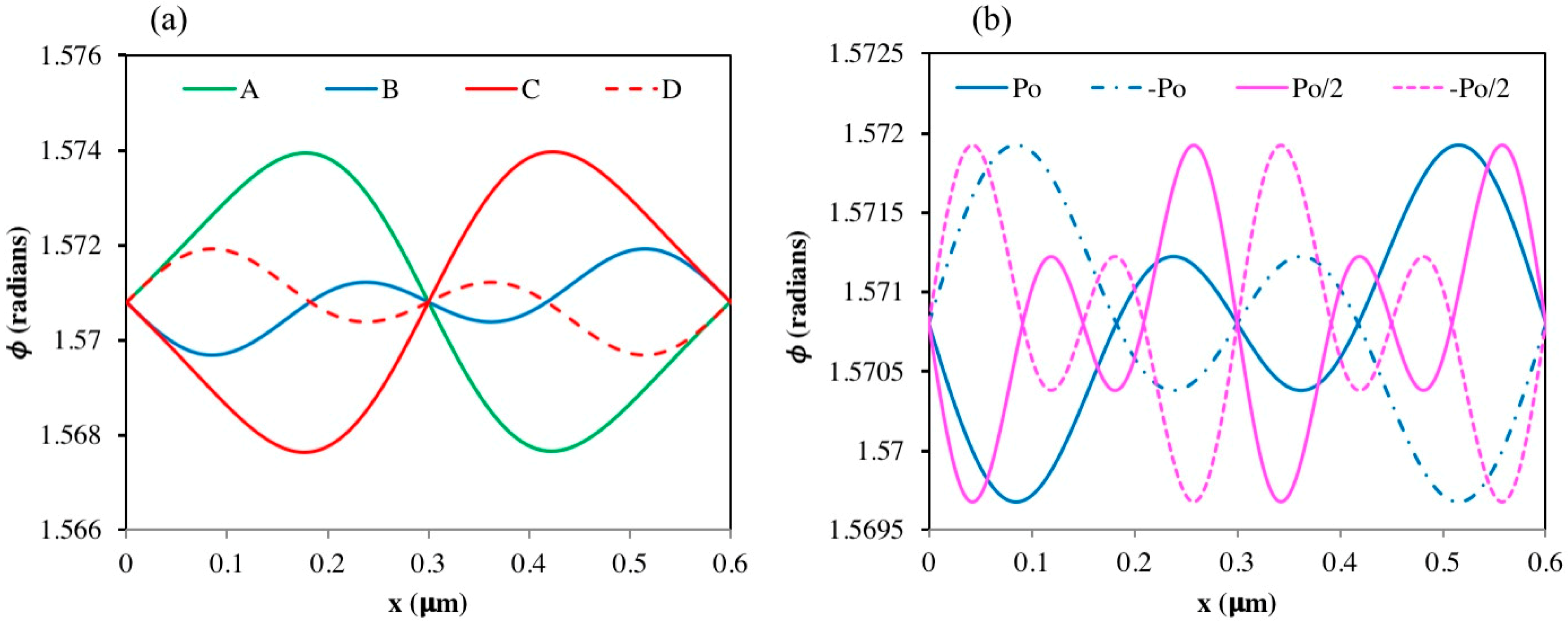
The surface normal angle, can be directly obtained through solving the governing shape equation, Equation (17). The generic features of the normal angle , its magnitude, and its periodicity are the three key outputs of the model. The two significant parameters influencing are the helix pitch P0, and the scaled anchoring coefficients and , which affect the periodicity and the magnitude of , correspondingly. Theoretically, and give two degrees of freedom to the governing equation. But, for small anchoring coefficients and constant helix pitch, the shape of is only a function of the anchoring ratio, . The plot of normal angle as a function of the distance “x”, corresponding to the points A, B, C, and D, is shown in Figure 3a. As expected, the periodicity equals the half pitch, P0/2, and the amplitude shows a slight deviation, . Figure 3b shows the effect of helix pitch on the normal angle for the particular point B at three different values of helix pitch P0, P0/2, and −P0/2. The helix pitch does not influence the amplitude’s span of normal angle, but it changes the periodicity of the normal angle. By reducing the helix pitch to half, a more squeezed normal angle profile can be observed. The sign of P0 reflects the normal angle profile with respect to . It should be noted that we can estimate the behavior of curvature by checking the slope of as .
The surface profile is then obtained from
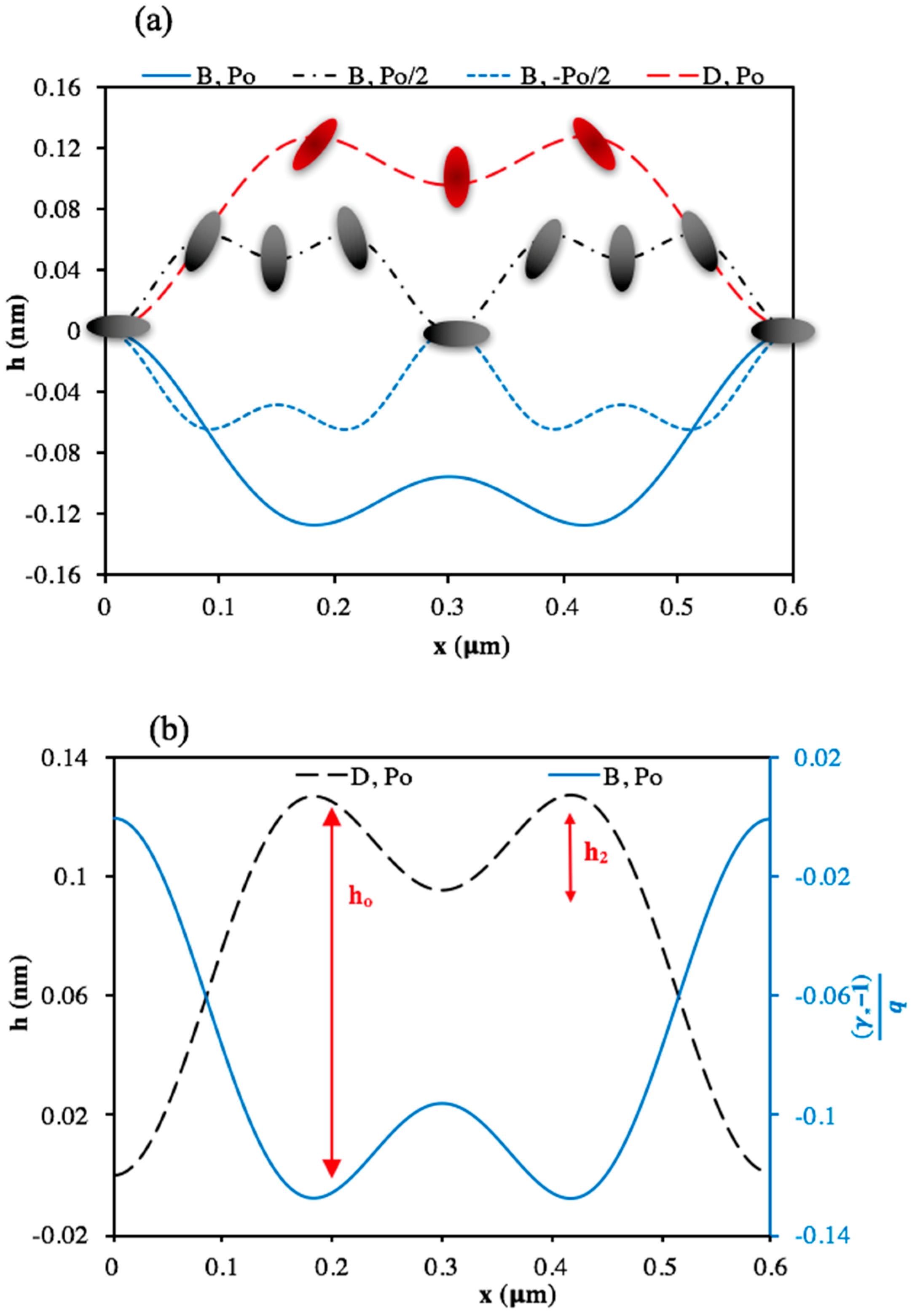
Figure 4a shows typical surface profiles h(x) and corresponding energy profile for the point B and point D. As shown in Figure 4a, increasing P0 results in both higher periodicity and magnitude. We can clearly see that the surface relief profiles of points B and D exhibit the mirror symmetry, while changing the sign of P0 result in the same mirror symmetry. These surface undulations can be validated with the two-length-scale surface modulations observed in a sheared CLC cellulosic films [25]. The two different scale periodical gratings include a primary set of bands perpendicular to the shear direction, and a smoother texture characterized by a secondary periodic structure containing “small” bands. It has been shown that the development and periodicities of the small bands are mainly ruled by the CLC characteristics. The chirality of CLC can therefore be mainly responsible for the formation of the secondary bands. The model can be also validated with the two-scale surface pattern of the Queen of the Night tulip [11], where for this specimen the ratio of amplitudes are h2/h0 = 0.01, and corresponding wavelength is λ = 1.2 μm.
Figure 4b shows the scaled energy profile, , in comparison with the surface profile for point B. The scaled energy profile gives the similar plot as the surface relief.
If we denote the parametric vector as , then becomes a function depending on two variables, the vector and the helix pitch P0. Within a linear regime , the following identities holds true:
This identity formulates the symmetric property of surface relief, and its relation to surface energy. Figure 4b is a clear demonstration of symmetry and scaling laws formulated in Equations (19a,b): if we compare B and D we have mirror symmetry and if we plot the anchoring energy of B we would see the same plot as the surface relief: .
Another important parameter that categorizes the shape of surface relief is the ratio between its two wavelengths. The origin of the two scales can be revealed through the linear theory, which gives the signed amplitudes of and (the nomenclature is defined in Figure 4b) as a function of anchoring ratio, :
and are defined as the two mode transition lines. Line , which gives a four-wave profile within one period corresponds to the condition (, ). Line , which gives a two-wave profile within one period corresponds to the condition (, ). In addition, if , then such that , also gives a two-wave profile.
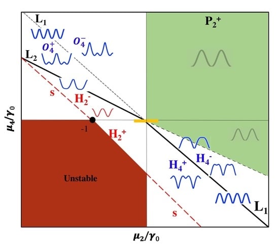
Figure 2b shows the general phase diagram of h-profiles in the parametric plane. As shown in the figure, the transition lines L1 and L2 are the critical lines across which surface relief changes its shape. We identify line L1 as a resonant line with the maximum interaction between quadratic and quartic anchoring effects.
The computations show that h-profile is centrally symmetrical with respect to original point, which can be observed in Figure 2b. As summarized as in Table 1, there are mainly three types of surface wrinkling patterns. It should be noted that there is no difference between O4+ and O4− as the patterns shown in one region are just a phase shift of the other; the same applies to H4+ and H4−. However, there is a difference between regions and due to the existence of a small plateau shown in the pattern computed along the two lines: and . This small plateau corresponds to the discontinuity of two capillary vectors diagram which will be discussed later.
Results above are considered within one period. Nomenclature: O (oblique), P (planar), and H (homeotropic) refer to the type of anchoring. The Li’s refer to transition lines; see text.
Table 1 summarizes the main four types of surface relief profiles. Region and both give four waves within one period. The difference is that four waves are identical on line . Region and both give two waves within one period, so is equal to 0. The difference between these two modes is that region gives very smooth surface geometry while region gives sharp peaks on the surface profile.
4.2. Surface Curvature
In this subsection we present, discuss, and characterize the surface curvature obtained from direct numerical simulations of the governing equations, and from a new and highly accurate linear model.
The surface behavior is not only affected by the magnitude of the surface relief, but also by the surface curvature. The curvature can be computed directly by two equivalent forms:
The first computing method in Equation (21) is exactly based on the governing Equation (17). Considering that for small values of anchoring coefficients, the resistant term is mainly controlled by isotropic energy , we obtain the resistant term denoted in Equation (17), . So, the linear approximation of curvature reads
where denotes the linear approximation of curvature assuming that . The analytical expression for the linear approximation of the surface relief is proposed in Appendix D. By assuming , we can also obtain another approximation for the surface curvature. It can be easily found that as we made similar assumptions to approximate the surface curvature based on Equation (21).
A more sophisticated approximation of curvature can be derived without linearizing the governing equation:
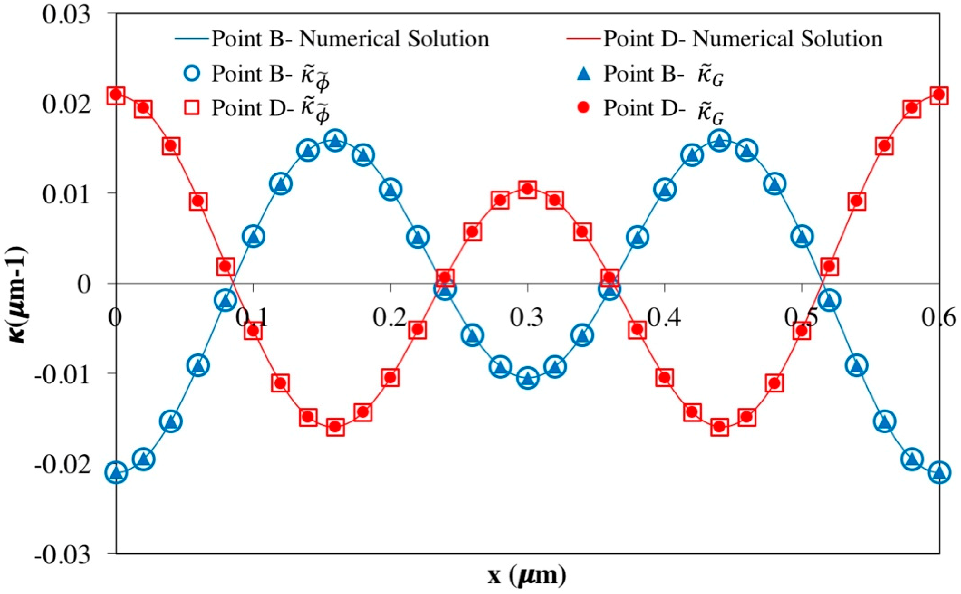
As illustrated in Figure 5, the linear approximation of curvature obtained by Equation (22) and from Equation (23) provides a very good approximation of curvature. As the curvature includes the explicit and simple expression, it allows us to mathematically derive more feasible relations to characterize the formation of the surface relief.
4.3. Surface Energy
Understanding surface energy behavior is another perspective in realizing the surface profile which helps us to establish an energy transfer mechanism from the anchoring energy of a flat surface into a wrinkled surface. For sufficient small values of the anchoring coefficients, as the normal angle profile is fluctuating around with a very small amplitude, an explicit relation between the linearized surface profile and the total surface energy can be estimated based on the linear approximation:
where () is the scaled anisotropic anchoring energy, and is the scaled surface relief. This correlation is detected in Figure 4b where h and are essentially identical for the small anchoring coefficients. This simple expression implies an essential physical phenomenon. The expression, Equation (24) verifies that zero anisotropic surface energy results in a flat surface (h = 0). As the result, based on the expression, the anchoring energy is the driving force contributing to the surface relief, which is in accordance with the previous findings [22]. Moreover, the expression confirms the expected insight that the uppermost surface area contain the highest surface energy.
4.4. Capillary Pressures
As mentioned above, the three main contributions in the capillary pressure are (1) : dilation pressure (Laplace pressure), : rotation pressure (Herrings pressure), : director curvature which is the anisotropic pressure due to the preferred orientation (see Equation (16)). is the driving forces to wrinkle the interface. The explicit expansion of Equation (16) in terms of yields:
As all the pressures are scaled by isotropic tension γ0, they have the same unit as curvature. It should be noted that based on theory .
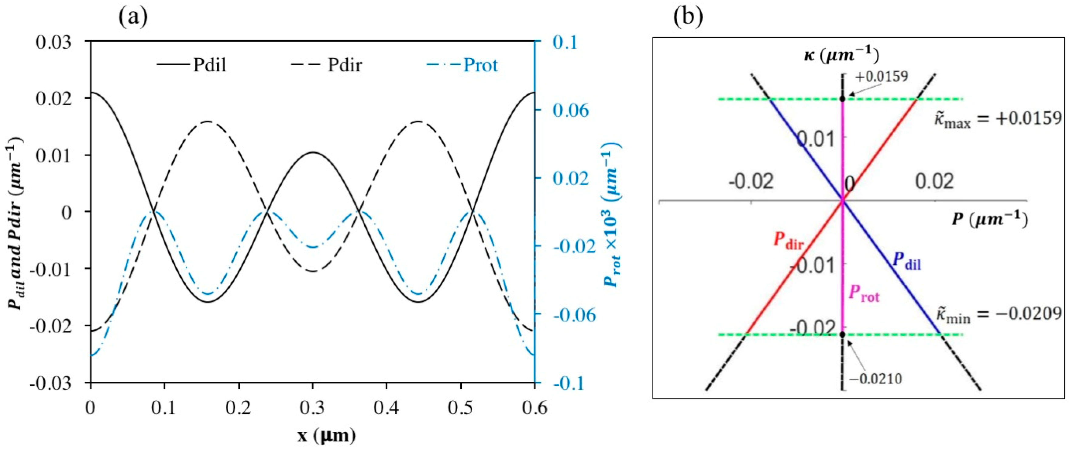
Figure 6a shows the wrinkling mechanism through the capillary pressures changes along x. The three scaled pressure contributions are plotted as function of “x” for the particular point B. As shown in the figure, the capillary pressures cancel each other out maintaining the summation at zero. The important observation from these pressure profiles is that and are always out-of-phase, while is always negative. These outcomes, and can be also interpreted from the linear model. Figure 6a also denotes that is two orders of magnitude smaller than and . This phenomenon confirms that is the formation source of wrinkling, annihilated by inducing area change and area rotation. Another observation from the linear model is that has the similar expression of curvature, . This similarity encourages us that capillary pressures can be also analyzed in the frame. Figure 6b shows the variation of curvature profile with respect to the capillary pressures. We can realize from the figure that in the linear region and for the constant P0, each capillary pressure only lay on intrinsic curves independent of the anchoring coefficients. The linear approximation gives the intrinsic curves (see Appendix E for the details):
The relations approve that helix pitch P0 is the only parameter affecting the intrinsic curves. Equation (26) implies that the intrinsic curves obtained for - P0 show the central symmetry. Variations in anchoring coefficients do not impose any influence on the intrinsic curves, they only change the arc-length of the intrinsic curves (denoted by ). The analytical expression of the arc-length for the intrinsic curves can be obtained by
where . If we denote , , and , then we denote and , considering the approximation curvature, (Equation (22)), the interval of can be found by
These findings denote that the span of curvature is associated with the anchoring coefficients, and ideally exhibits a linear correlation with 1/P0. So, we expect that if the helix pitch is increased to 2P0 under the same anchoring condition, the span of curvature would reduce to half. Figure 6b illustrates the numerical solutions for director, dilation, and rotation pressures obtained by Equation (25) in comparison with the intrinsic lines defined by Equation (26). We can observe that there are no considerable deviations between the director pressures and the intrinsic lines approximated by the linear model. As shown in Figure 6b, the span of actual curvature is in accordance with the minimum and maximum values of curvature computed by Equations (30) and (31), which confirms that the linear approximation is validated within the linear region (small anchoring coefficients).
In partial summary, in this subsection we have shown (i) the key balancing pressures are the Laplace and director pressures (Figure 6); (ii) quadratic curvature contributions are proportional to the pitch, the curvature–pressure relations follow intrinsic curves (Equation (26)) whose lengths are affected by anchoring, such that lower anchoring (higher anchoring) decreases (increases) their lengths (Equations (27)–(31)).
4.5. Capillary Vectors
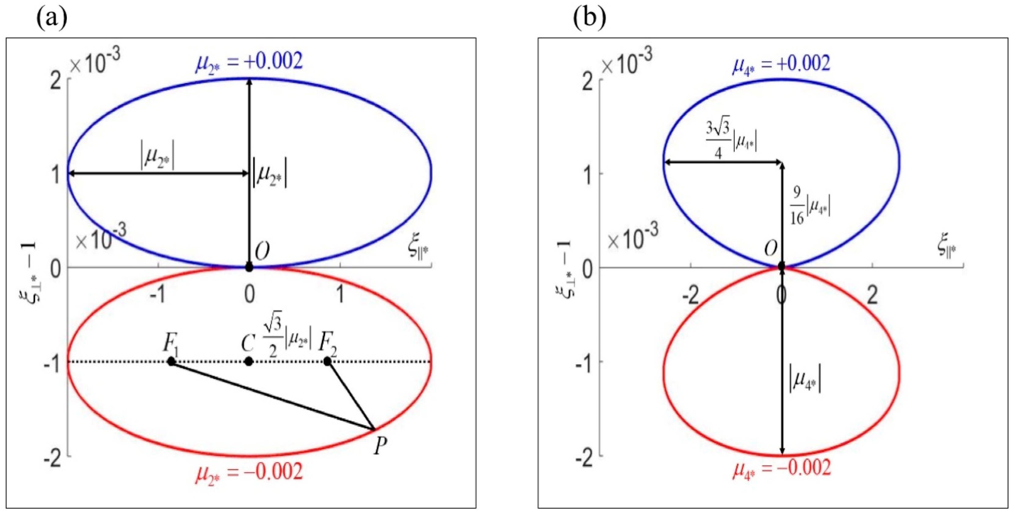
The behavior of the capillary vectors can give another perspective to analyze the surface wrinkling. If we assume that , then the magnitude of two capillary vectors and naturally satisfy
denotes the magnitude of the capillary vector, . From this equation, we can read an ellipse with eccentricity which is independent of anchoring coefficient . The two capillary vectors change proportionally; oscillates around with an amplitude of , while oscillates around zero with amplitude of . This ellipse with invariant shape can provide a clear physical explanation to understand how capillary vectors are formed. Figure 7a illustrates the plots of the ellipse equation for the anchoring coefficient . Considering that the CLC surface is differentiable, we can introduce two foci ( and , defined by in Figure 7b) such that every point in the vector diagram is restrained by . When , two foci are very close to each other, giving that . Ellipse becomes a circle with a radius of , which can be considered as a point. From Figure 7a we can also observe that only reaches its extrema when vanishes. This phenomenon corresponds to . However, when reaches its extrema, does not vanish as isotropic surface tension prevents to be reduced to zero.
The solution to ellipse equation yields
These are explicit algebraic relations between and . Recall that the capillary vectors and the normal angle are related by
Replacing with from Equation (33), the normal angle can be expressed only in term of (see Appendix F):
Equation (35) clarifies the source of fluctuation; the perturbation , is imposed onto the normal angle profile due to the presence of , which is fixed by the ellipse equation.
If we assume that , the magnitude of two capillary vectors and satisfy
This equation reads a teardrop curve. Figure 7b illustrates the plots of the teardrop equation for the anchoring coefficient . The main parameters defining this teardrop curve are given in Figure 7b. Similar to the ellipse curves shown in Figure 7a, the magnitude of does not change the shape of teardrops, while it controls the size of the teardrop curves. It should be noted that the teardrop curves are not continuous at the original point (Point O shown in Figure 7b). Both the ellipse and teardrop curves show a symmetry by changing the sign of the anchoring coefficients, and shrink to zero as the anchoring coefficients go to zero.
5. Conclusions
This paper presents a rigorous model based on nonlinear nemato-capillarity shape equation and its linear approximation to describe the main formation mechanism of two-length scale surface wrinkling formed at the CLC/air interface. The role of three capillary pressure contributions (dilation, rotation, and director curvature) on the formation of surface curvature have been elucidated and the effect of the helix pitch and the anchoring coefficients has been characterized. The linear approximation provides a simple model to describe wrinkling behavior with high accuracy and less computation when the two anchoring coefficients are very small. The linear approximation can also serve as the main criteria to classify the type of surface relief. The key mechanism driving surface wrinkling is identified and discussed through the two perspectives: capillary pressures and capillary vectors. Moreover, the surface normal is expressed by the capillary pressures, whose summation must maintain at zero, serving as the constraint to the system. The proposed new model and its linear approximation augment previous models dedicated to understand and mimic complex surface patterns observed at the free surface of synthetic and biological chiral nematic liquid crystals, chiral polymer solutions, surfactant-liquid crystal surfaces and membranes, and in frozen biological plywoods. The present results can inspire design and fabrication of complex surface patterns with the possible potentials in optical, high friction, and thermal applications.
Author Contributions
The manuscript was written through contributions from Z.W and P.R. Review & editing, A.D.R and P.R. All authors have approved the final version of manuscript.
Funding
A part of this work was supported by Le Fonds Quebecois de la Recherche sur la Nature et les Technologies (FRQNT) Postdoctoral Research Scholarship Grant Number 205888.
Acknowledgments
Authors thank the Natural Science and Engineering Research Council of Canada (NSERC) and Le Fonds Quebecois de la Recherche sur la Nature et les Technologies (FRQNT) for financial support of this research.
Conflicts of Interest
The authors declare no conflict of interest.
Appendix A. Cahn-Hoffman Capillary Vector
The purpose of Appendix A is to derive the Cahn-Hoffman capillary vectors that are being used in the main text.
Cahn-Hoffman capillary vector is defined as the gradient of the scalar field
where is the position vector, and . . Notice that :
t is the unit tangent, k is the outward unit normal, and n is director vector (see Figure A1). Equation (A3) yields the two components of capillary vectors (scaled by ):
Figure A1.
Nomenclature of normal angle and vectors in Cartesian coordinates.

Appendix B. Capillary Pressures
The purpose of Appendix B is to drive the explicit expressions of capillary pressures.
Denote linear operator for simplicity, and introduce an identity such that:
Equation (A6) holds due to . We can introduce another identity:
Three capillary pressures can be derived by:
Therefore, the surface curvature is written as:
Equation (A11) is the general curvature equation for .
Appendix C. Governing Equation
The purpose of Appendix C is to show how we obtained governing equation and the uniqueness of its solution within the linear region.
A trivial solution to is that is a constant. Here, we need to consider whether this solution can be true. Inserting boundary condition such that , we get , where is the unit vector along y axis:
Take the square of (A12) on both side, we obtain:
This equation does not hold true when both and are greater than 0. Therefore, is not a constant. Equation (A11) is an ODE where we can solve for and subsequently obtain :
Here, we introduce two terms, and as the driving and resistant terms in the formation of the surface wrinkles that can be defined by:
Therefore, Equation (A14) becomes the governing equation that is going to be solved to obtain . It is easy to find that:
where the last term only exists when . Thus, for very small and , we can conclude that and it is bounded. So, Equation (A14) has a unique solution.
Appendix D. Linear Theory
The purpose of Appendix D is to show how the linear theory is formed and the application to surface parameters by using linear theory presented in section (3.2).
We consider the first linear theory by simply assuming that . Then, governing equation provides a simple expression of surface curvature:
However, we could not obtain an explicit expression for the linearized surface relief using this approximated curvature. As we observed that is very small compared to , the trivial solution can be obtained using an approximation such that .
By using the Monge parametrization, the surface equation can be expressed by:
Then we multiply by on both side of :
By integrating on both side with respect to x, we obtain:
Replacing , we find the linearized surface relief:
Once we get , we can also obtain other surface parameters:
Omitting the denominator in Equation (A18), we can obtain an approximation curvature from the linearized governing equation. We can also approximate surface curvature by :
Notice that Equations (A25) and (A26) are equivalent.
Equation (A23) also gives a simple explicit form to approximate :
We can also detect the two length scales and by finding the extrema of Equation (A27). There are three conditions satisfying (A27): (i) , (ii) and (iii) . Condition (i) yields that , while the other two conditions yield that and , respectively. Therefore, we can introduce the following scaling law:
Equation (A28) indicates that the only parameter which is defined as the anchoring ratio determines the characteristic shape of surface relief.
Appendix E. Relations
The purpose of Appendix E is to demonstrate the relationship between capillary pressures and curvature by using linear theory presented in section (3.3).
Applying linear theory into three capillary pressures, we obtain approximated relations in explicit forms:
Using the linear model, we can find the approximated interval of curvature :
Since , we need to examine whether local extremum can be achieved or not. Considering function as:
This function describes how the x axis of local extrema changes with .
When local extremum of is not achieved, there should be . This gives:
In this case, two critical values of for would be:
The minimum and maximum of can be expressed as:
If , local extremum becomes:
Let and . Summarizing all the results above, we can find the span of curvature :
For example, if we choose point A, we have . Then, , , , and subsequently , where numerical solution gives that . As the linear theory only deviates 0.6% from exact solution, the error can be ignored.
The span in plot can be calculated by arc-length equation:
Using the fact that:
We can compute the arc-lengths corresponding to the three capillary pressures:
Using Equation (A42) to Equation (A44), we can compute the arc-length of each curve.
Appendix F. Capillary Vectors
The purpose of Appendix F is to derive the equations related to capillary vectors that are being used in section (3.4).
The following equation holds for capillary vectors:
The projection of capillary vector along direction reduces Equation (A45) to:
Replacing with from ellipse equation (assuming that ), we obtain:
Considering that , we can use symmetry role for evaluating the cases where . Within the linear region, we can integrate on both side of Equation (A47) and obtain:
There are two depending on the positive or the negative sign showed inside the integrand of Equation (A48). The explicit expression of reads:
Assume that , and satisfy:
We can find that the extrema of are 0 and . As shows symmetry, we only consider the positive branch and find the derivative:
The non-trivial extrema of occur at:
It should be noticed that Equation (A51) is singular at , implying that the plot is not continuous at the point where .
References
- Vignolini, S.; Moyroud, E.; Glover, B.J.; Steiner, U. Analysing photonic structures in plants. J. R. Soc. Interface 2013, 10. [Google Scholar] [CrossRef] [PubMed]
- Willcox, P.J.; Gido, S.P.; Muller, W.; Kaplan, D.L. Evidence of a cholesteric liquid crystalline phase in natural silk spinning processes. Macromolecules 1996, 29, 5106–5110. [Google Scholar] [CrossRef]
- Sharma, V.; Crne, M.; Park, J.O.; Srinivasarao, M. Structural Origin of Circularly Polarized Iridescence in Jeweled Beetles. Science 2009, 325, 449–451. [Google Scholar] [CrossRef] [PubMed]
- Tan, T.L.; Wong, D.; Lee, P. Iridescence of a shell of mollusk Haliotis Glabra. Opt. Express 2004, 12, 4847–4854. [Google Scholar] [CrossRef] [PubMed]
- Parker, A.R. Discovery of functional iridescence and its coevolution with eyes in the phylogeny of Ostracoda (Crustacea). Proc. R. Soc. B Biol. Sci. 1995, 262, 349–355. [Google Scholar]
- Parker, A.R.; Martini, N. Diffraction Gratings in Caligoid (Crustacea: Copepoda) Ecto-parasites of Large Fishes. Mater. Today: Proc. 2014, 1, 138–144. [Google Scholar] [CrossRef]
- Sharma, V.; Crne, M.; Park, J.O.; Srinivasarao, M. Bouligand Structures Underlie Circularly Polarized Iridescence of Scarab Beetles: A Closer View. Mater. Today: Proc. 2014, 1, 161–171. [Google Scholar] [CrossRef]
- Vukusic, P.; Sambles, J.R.; Lawrence, C.R. Structural colour—Colour mixing in wing scales of a butterfly. Nature 2000, 404, 457. [Google Scholar] [CrossRef]
- Gould, K.S.; Lee, D.W. Physical and ultrastructural basis of blue leaf iridescence in four Malaysian understory plants. Am. J. Bot. 1996, 83, 45–50. [Google Scholar] [CrossRef]
- Graham, R.M.; Lee, D.W.; Norstog, K. Physical and Ultrastructural Basis of Blue Leaf Iridescence in 2 Neotropical Ferns. Am. J. Bot. 1993, 80, 198–203. [Google Scholar] [CrossRef]
- Whitney, H.M.; Kolle, M.; Andrew, P.; Chittka, L.; Steiner, U.; Glover, B.J. Floral Iridescence, Produced by Diffractive Optics, Acts As a Cue for Animal Pollinators. Science 2009, 323, 130–133. [Google Scholar] [CrossRef] [PubMed]
- Urbanski, M.; Reyes, C.G.; Noh, J.; Sharma, A.; Geng, Y.; Jampani, V.S.R.; Lagerwall, J.P.F. Liquid crystals in micron-scale droplets, shells and fibers. J. Phys. Condens. Matter 2017, 29, 133003. [Google Scholar] [CrossRef] [PubMed] [Green Version]
- Mitov, M. Cholesteric liquid crystals in living matter. Soft Matter 2017, 13, 4176–4209. [Google Scholar] [CrossRef] [PubMed]
- Rey, A.D. Liquid crystal models of biological materials and processes. Soft Matter 2010, 6, 3402–3429. [Google Scholar] [CrossRef]
- Bouligan, Y. Twisted Fibrous Arrangements in Biological-Materials and Cholesteric Mesophases. Tissue Cell 1972, 4, 189–217. [Google Scholar] [CrossRef]
- Neville, A.C. Biology of Fibrous Composites: Development Beyond the Cell Membrane; Cambridge University Press: New York, NY, USA, 1993; p. vii. 214p. [Google Scholar]
- Rey, A.D.; Herrera-Valencia, E.E.; Murugesan, Y.K. Structure and dynamics of biological liquid crystals. Liq. Cryst. 2014, 41, 430–451. [Google Scholar] [CrossRef]
- Rey, A.D.; Herrera-Valencia, E.E. Liquid crystal models of biological materials and silk spinning. Biopolymers 2012, 97, 374–396. [Google Scholar] [CrossRef]
- Murugesan, Y.K.; Pasini, D.; Rey, A.D. Self-assembly Mechanisms in Plant Cell Wall Components. J. Renew. Mater. 2015, 3, 56–72. [Google Scholar] [CrossRef]
- Canejo, J.P.; Monge, N.; Echeverria, C.; Fernandes, S.N.; Godinho, M.H. Cellulosic liquid crystals for films and fibers. Liq. Cryst. Rev. 2017, 5, 86–110. [Google Scholar] [CrossRef]
- Rofouie, P.; Alizadehgiashi, M.; Mundoor, H.; Smalyukh, I.I.; Kumacheva, E. Self-Assembly of Cellulose Nanocrystals into Semi-Spherical Photonic Cholesteric Films. Adv. Funct. Mater. 2018, 28. [Google Scholar] [CrossRef]
- Rofouie, P.; Pasini, D.; Rey, A.D. Nano-scale surface wrinkling in chiral liquid crystals and plant-based plywoods. Soft Matter 2015, 11, 1127–1139. [Google Scholar] [CrossRef] [PubMed]
- Rofouie, P.; Pasini, D.; Rey, A.D. Nanostructured free surfaces in plant-based plywoods driven by chiral capillarity. Colloids Interface Sci. Commun. 2014, 1, 23–26. [Google Scholar] [CrossRef] [Green Version]
- Rofouie, P.; Pasini, D.; Rey, A.D. Tunable nano-wrinkling of chiral surfaces: Structure and diffraction optics. J. Chem. Phys. 2015, 143, 114701. [Google Scholar] [CrossRef] [Green Version]
- Fernandes, S.N.; Geng, Y.; Vignolini, S.; Glover, B.J.; Trindade, A.C.; Canejo, J.P.; Almeida, P.L.; Brogueira, P.; Godinho, M.H. Structural Color and Iridescence in Transparent Sheared Cellulosic Films. Macromol. Chem. Phys. 2013, 214, 25–32. [Google Scholar] [CrossRef]
- Sharon, E.; Roman, B.; Marder, M.; Shin, G.S.; Swinney, H.L. Mechanics: Buckling cascades in free sheets—Wavy leaves may not depend only on their genes to make their edges crinkle. Nature 2002, 419, 579. [Google Scholar] [CrossRef]
- Aharoni, H.; Abraham, Y.; Elbaum, R.; Sharon, E.; Kupferman, R. Emergence of Spontaneous Twist and Curvature in Non-Euclidean Rods: Application to Erodium Plant Cells. Phys. Rev. Lett. 2012, 108, 238106. [Google Scholar] [CrossRef]
- Rofouie, P.; Pasini, D.; Rey, A.D. Multiple-wavelength surface patterns in models of biological chiral liquid crystal membranes. Soft Matter 2017, 13, 541–545. [Google Scholar] [CrossRef]
- Rofouie, P.; Pasini, D.; Rey, A.D. Morphology of elastic nematic liquid crystal membranes. Soft Matter 2017, 13, 5366–5380. [Google Scholar] [CrossRef]
- Rofouie, P.; Wang, Z.; Rey, A.D. Two-wavelength wrinkling patterns in helicoidal plywood surfaces: Imprinting energy landscapes onto geometric landscapes. Soft Matter 2018, 14, 5180–5185. [Google Scholar] [CrossRef]
- Cheong, A.G.; Rey, A.D. Cahn-Hoffman capillarity vector thermodynamics for curved liquid crystal interfaces with applications to fiber instabilities. J. Chem. Phys. 2002, 117, 5062–5071. [Google Scholar] [CrossRef]
- Rapini, A.; Papoular, M. Distorsion d’une lamelle nématique sous champ magnétique conditions d’ancrage aux parois. J. Phys. Colloq. 1969, 30, C4-54–C4-56. [Google Scholar] [CrossRef]
- Rey, A.D. Capillary models for liquid crystal fibers, membranes, films, and drops. Soft Matter 2007, 3, 1349–1368. [Google Scholar] [CrossRef]
- Belyakov, V.A.; Shmeliova, D.V.; Semenov, S.V. Towards the restoration of the liquid crystal surface anchoring potential using Grandgean-Cano wedge. Mol. Cryst. Liq. Cryst. 2017, 657, 34–45. [Google Scholar] [CrossRef]
- Rey, A.D. Nemato-capillarity theory and the orientation-induced Marangoni flow. Liq. Cryst. 1999, 26, 913–917. [Google Scholar] [CrossRef]
- Rey, A.D. Marangoni flow in liquid crystal interfaces. J. Chem. Phys. 1999, 110, 9769–9770. [Google Scholar] [CrossRef]
- Eelkema, R.; Pollard, M.M.; Katsonis, N.; Vicario, J.; Broer, D.J.; Feringa, B.L. Rotational reorganization of doped cholesteric liquid crystalline films. J. Am. Chem. Soc. 2006, 128, 14397–14407. [Google Scholar] [CrossRef] [PubMed]
- Yang, X.G.; Li, J.; Forest, M.G.; Wang, Q. Hydrodynamic Theories for Flows of Active Liquid Crystals and the Generalized Onsager Principle. Entropy 2016, 18, 202. [Google Scholar] [CrossRef]
- Forest, M.G.; Wang, Q.; Zhou, R.H. Kinetic theory and simulations of active polar liquid crystalline polymers. Soft Matter 2013, 9, 5207–5222. [Google Scholar] [CrossRef]
- Brand, H.R.; Pleiner, H.; Svensek, D. Dissipative versus reversible contributions to macroscopic dynamics: The role of time-reversal symmetry and entropy production. Rheol. Acta 2018, 57, 773–791. [Google Scholar] [CrossRef]
- Rey, A.D. Theory of linear viscoelasticity of chiral liquid crystals. Rheol. Acta 1996, 35, 400–409. [Google Scholar] [CrossRef]
- Rey, A.D. Theory of linear viscoelasticity of cholesteric liquid crystals. J. Rheol. 2000, 44, 855–869. [Google Scholar] [CrossRef]
- Hoffman, D.W.; Cahn, J.W. Vector Thermodynamics for Anisotropic Surfaces 1. Fundamentals and Application to Plane Surface Junctions. Surf. Sci. 1972, 31, 368–388. [Google Scholar] [CrossRef]
- Rey, A.D. Mechanical model for anisotropic curved interfaces with applications to surfactant-laden liquid-liquid crystal interfaces. Langmuir 2006, 22, 219–228. [Google Scholar] [CrossRef] [PubMed]
- Fedorov, F.I. Covariant description of the properties of light beam. J. Appl. Spectrosc. 1965, 2, 344–351. [Google Scholar] [CrossRef]
- Sihvola, A.H. Institution of Electrical Engineers. In Electromagnetic Mixing Formulas and Applications; Institution of Electrical Engineers: London, UK, 1999; p. xii. 284p. [Google Scholar]
Figure 1.
Schematic of a cholesteric liquid crystals (CLC) and surface structures. H is the helix unit vector, and P0 is the pitch. The surface director has an ideal cholesteric twist in the bulk. The helix uncoiling near the surface creates a bend and splay planar (2D) orientation and surface undulations of nanoscale relief h(x) with micron range wavelength P0/2. Adapted from [22].

Figure 2.
(a) Parametric space in terms of the two anchoring coefficients obtained using Equation (17). Two characteristic lines (blue dash-dot) and (purple dash-dot) indicate wrinkling mode transitions, . The subscript numbers indicate how many waves there are within one period. P, O, H represent planar, oblique, homeotropic anchoring, respectively. The thermodynamic line, S, passing point illustrates the points where it ends on and axes. A (+0.002, +0.001), B (−0.002, +0.0015), C (−0.002, −0.001), and D (+0.002, −0.0015) are four representative points in region , , , and , respectively. The region below the dotted S line implies an unstable state because the surface tension is negative. (b) Surface relief profile in the parametric space obtained using Equation (17). The anchoring coefficients correspond to all computed curves are less than 0.01.

Figure 3.
Normal angle profile. (a) The normal angle profiles corresponding to the points A, B, C, and D as illustrated in Figure 2a: A (green; mode ), B (blue, mode ), C (red, full line, mode ), and D (red, dashed line, mode . (b) The normal angle profile for the point B at different helix pitch values of P0, −P0, P0/2 and −P0/2, where P0 = 1.2 μm.

Figure 4.
Mirror symmetries observed in surface relief profiles. (a) The surface relief profiles at point B with different helix pitches are given by the two blue curves and the black curve. The red curve gives the surface relief profile at point D. The red and black ellipsoids depict the director orientation for point B with P0/2 and point D with P0, respectively. These ellipsoids show where the surface extrema occur for planar, homeotropic, and oblique anchoring. (b) The surface profile at point D and scaled energy profile at point B. This figure indicates that there is similarity between surface relief profile and energy profile. The helix pitch is.

Figure 5.
Surface curvature profiles computed numerically and with the two approximation methods: and . Blue and red solid lines are the numerical solutions solved from governing equation for point B and D, respectively. Blue hollow circles and blue filled triangles represent the data points of computed and at point B, respectively. Red hollow squares and red filled circles represent the data points of computed and at point D, respectively. As the both approximations and are identical, the filled circles and triangles are superimposed on hollow squares and circles. The helix pitch is P0 = 1.2 μm.

Figure 6.
Capillary pressure profile. (a) Three components of capillary pressures with respect to x axis for the point B. Black real line, black dash line, and blue dot line represent dilation pressure, director pressure, and rotation pressure, respectively. (b) Curvature–Pressure plot at point B. Red, blue, and purple lines represent the numerical solutions to director pressure, dilation pressure, and rotation pressure, respectively. Black dash lines are the intrinsic lines defined by Equation (26). Green dash lines are the span of curvature computed by Equations (30) and (31). Two black points are where the span of numerical solution for curvature ends. The helix pitch is .

Figure 7.
Plots of capillary vector components under two limiting anchoring coefficient values. (a) results in an ellipse. (b) . This results in a teardrop curve. The sign of anchoring coefficient imposes a mirror symmetry. The axes of the loops are determined by the anchoring coefficients.
Figure 7.
Plots of capillary vector components under two limiting anchoring coefficient values. (a) results in an ellipse. (b) . This results in a teardrop curve. The sign of anchoring coefficient imposes a mirror symmetry. The axes of the loops are determined by the anchoring coefficients.


Table 1.
Surface wrinkling patterns in different regions of the parametric space .
| Region | Total Wave Number | h2/h0 |
|---|---|---|
| 4 | ≠1 | |
| 4 | =1 | |
| 2 | =0 | |
| 2 | =0 |
© 2019 by the authors. Licensee MDPI, Basel, Switzerland. This article is an open access article distributed under the terms and conditions of the Creative Commons Attribution (CC BY) license (http://creativecommons.org/licenses/by/4.0/).
Share and Cite
MDPI and ACS Style
Wang, Z.; Rofouie, P.; Rey, A.D. Surface Anchoring Effects on the Formation of Two-Wavelength Surface Patterns in Chiral Liquid Crystals. Crystals 2019, 9, 190. https://doi.org/10.3390/cryst9040190
AMA Style
Wang Z, Rofouie P, Rey AD. Surface Anchoring Effects on the Formation of Two-Wavelength Surface Patterns in Chiral Liquid Crystals. Crystals. 2019; 9(4):190. https://doi.org/10.3390/cryst9040190
Chicago/Turabian StyleWang, Ziheng, Pardis Rofouie, and Alejandro D. Rey. 2019. "Surface Anchoring Effects on the Formation of Two-Wavelength Surface Patterns in Chiral Liquid Crystals" Crystals 9, no. 4: 190. https://doi.org/10.3390/cryst9040190
Note that from the first issue of 2016, this journal uses article numbers instead of page numbers. See further details here.