Article

Convolutional Neural Networks for Crystal Material Property Prediction Using Hybrid Orbital-Field Matrix and Magpie Descriptors

1
School of Mechanical Engineering, Guizhou University, Guiyang 550025, China
2
Department of Computer Science and Engineering, University of South Carolina, Columbia, SC 29208, USA
3
Key Laboratory of Advanced Manufacturing Technology, Ministry of Education, Guiyang 550025, China
*
Author to whom correspondence should be addressed.
Crystals 2019, 9(4), 191; https://doi.org/10.3390/cryst9040191
Submission received: 9 March 2019 / Revised: 25 March 2019 / Accepted: 28 March 2019 / Published: 3 April 2019
(This article belongs to the Section Crystalline Materials)

Abstract

:
Computational prediction of crystal materials properties can help to do large-scale in-silicon screening. Recent studies of material informatics have focused on expert design of multi-dimensional interpretable material descriptors/features. However, successes of deep learning such as Convolutional Neural Networks (CNN) in image recognition and speech recognition have demonstrated their automated feature extraction capability to effectively capture the characteristics of the data and achieve superior prediction performance. Here, we propose CNN-OFM-Magpie, a CNN model with OFM (Orbital-field Matrix) and Magpie descriptors to predict the formation energy of 4030 crystal material by exploiting the complementarity of two-dimensional OFM features and Magpie features. Experiments showed that our method achieves better performance than conventional regression algorithms such as support vector machines and Random Forest. It is also better than CNN models using only the OFM features, the Magpie features, or the basic one-hot encodings. This demonstrates the advantages of CNN and feature fusion for materials property prediction. Finally, we visualized the two-dimensional OFM descriptors and analyzed the features extracted by the CNN to obtain greater understanding of the CNN-OFM model.

1. Introduction

In recent years, research on high-throughput experiments and high-throughput computational methods has made significant progress with the development of the Materials Genome Initiative (MGI). Keisuke Takahashi [1] et al. proposed a workflow of materials synthesis and design from first principle calculations and machine learning which pointed out the research pattern of material informatics. In particular, an increasing number of studies have applied machine learning (ML) algorithms for material property prediction [2]. Most of these studies first try to represent the materials in a certain way (also known as descriptor design or feature engineering), and then employ some popular machine learning algorithms to build predictive models for materials properties prediction such as band gaps, formation energy, melting temperature, critical temperature of superconductivity materials, etc. [3,4,5,6]. In short, current material informatics studies focus on the materials feature engineering combined with the application of standard machine learning algorithms. When designing materials descriptors, the first consideration is that the form of the descriptors should match machine learning algorithms, most of which can only accept one-dimensional numerical features. Secondly, the descriptor of materials should contain as much information as possible in some aspect related to materials property. Commonly used information includes elemental composition or structural information of the materials or molecule [7,8]. Third, the descriptor should have a certain interpretability from the physical or chemical perspective [9]. At present, the design of descriptors focuses more on the third aspect. Descriptors with physical/chemical interpretability tend to provide better guidance to quantifiable materials experiments [10]. From the machine learning point of view, the material properties prediction problem is mostly a regression problem since the target characteristic to be predicted is usually numeric values, e.g., formation energy of crystalline materials and atomization energy of molecular systems.
According to the dimensions, current descriptors can be classified into three categories: one-dimensional vector, two-dimensional matrix, and three-dimensional matrix. The simplest way to characterize a material is to encode it with a one-dimensional vector such as the one-hot encoding [11,12], which can be used to encode atomic composition or the spatial structure of a molecule. The well-known Magpie descriptor set [12] calculates a few statistics for each property of the elements in a given compounds, which allows it to integrate physical, chemical, electronic, ionic and basic properties of the material into one-dimensional vector features. Magpie features is a descriptor set designed to create quantitative representation that both uniquely defines each material in a data set and relates to the essential physics and chemistry that influences the property of interest [9,13], including material attributes of stoichiometric, elemental property statistics, electronic structure and ionization characteristic. For electronic structure attributes in Magpie features, it also includes electronic configuration information, such as the average fraction of electrons from the s, p, d, and f valence among all elements present. Magpie features are the most popular descriptors that can be calculated without the crystal structure information.
For two-dimensional descriptors, T. L. Pham et al. [14] proposed OFM (Orbital-field matrix) descriptors by first characterizing the atoms as one-dimensional vectors according to the electron configurations, and then adding the information of the number of nearest-neighbor atoms surrounding the central atom, the distance between atoms, the coordination number and so on. Each atom in the molecule is constructed as a two-dimensional matrix of fixed size and then finally the descriptor for the entire structure is obtained by averaging the descriptors of the atoms. Q. Zhou et al. [15] developed the Atom2Vec descriptor which uses a method similar to word embedding in natural language processing. Atom embedding of a single atom with fixed length are generated from a large data set (about 60,000 inorganic compounds) and then the atomic vectors are stacked into two-dimensional matrices according to the atomic composition of molecules when characterizing a molecule. CM descriptor [16] is also a commonly used two-dimensional descriptor, which mainly characterizes the 3D structure of molecules. The development of 3D descriptors for materials is rare. S. Kajita et al. [17] proposed R3DVS, a three-dimensional descriptor which contains field quantity information and rotation invariance in the molecular structure, which achieved comparable results with CM and SOAP descriptor [18] when they used 680 oxide datasets randomly selected from ICSD (Inorganic Crystal Structure Database) databases. Moreover, the ways of improving R3DVS descriptor are also proposed. A comprehensive survey of materials descriptors can be found in reference [7].
It is worth noting that currently there is a lot of research on materials descriptor design or feature engineering. However, recent successes of deep learning in computer vision, speech recognition, and machine translations have demonstrated that instead of relying on human-engineered features, the deep learning algorithms such as convolutional neural networks can achieve much better performance by learning hierarchical features from the raw data. Following this paradigm’s development, Cecen et al. [19] represented the microstructures of 5900 materials into three-dimensional matrices of 51 × 51 × 51 and then used simple convolution neural networks to extract and analyze the hidden features, which allowed them to explore the relationship between microstructures and material properties. Afterwards, they squeezed the features extracted by the CNN model into one-dimensional vectors and a machine learning algorithm was employed to predict the elastic properties of materials. In another work, Xie et al. [20] proposed a graph convolutional neural network model for property predictions of materials. However, their method can only be applicable to materials with known crystal structure information. On the other hand, conventional machine learning models usually need one dimensional feature vector representation to work properly. However, converting two-dimensional or three-dimensional descriptors into one-dimensional vectors inevitably leads to loss of information, which may lead to performance degradation of the model.
Therefore, this paper proposed and applied a convolution neural network model to predict the formation energy of materials by using combining the two-dimensional OFM descriptors and Magpie features. The main contributions of this paper are as follows:
(1)
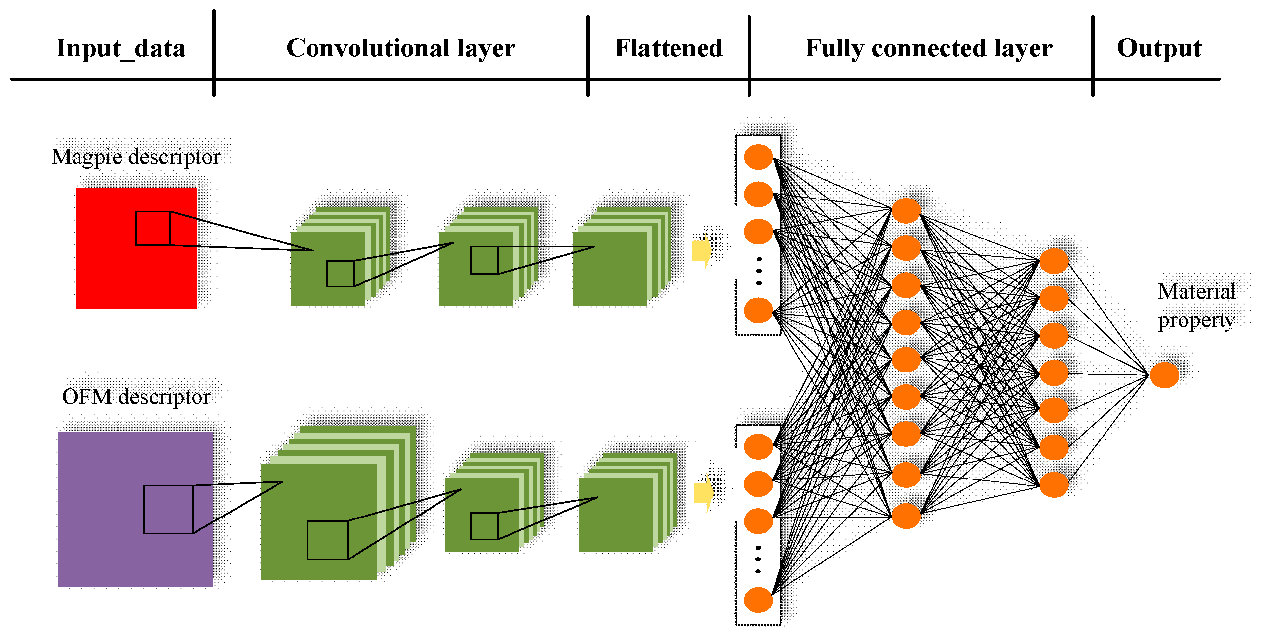
We proposed CNN-OFM-Magpie, a convolution neural network model for materials formation energy prediction by exploiting its hierarchical feature extraction capabilities and fusion of two different types of features.
(2)
We evaluated the performance of CNN-OFM and compared it with those of the regression prediction models based on conventional machine learning algorithms such as SVM, Random Forest, and KRR using OFM features and Magpie features, and showed the advantages of the CNN model.
(3)
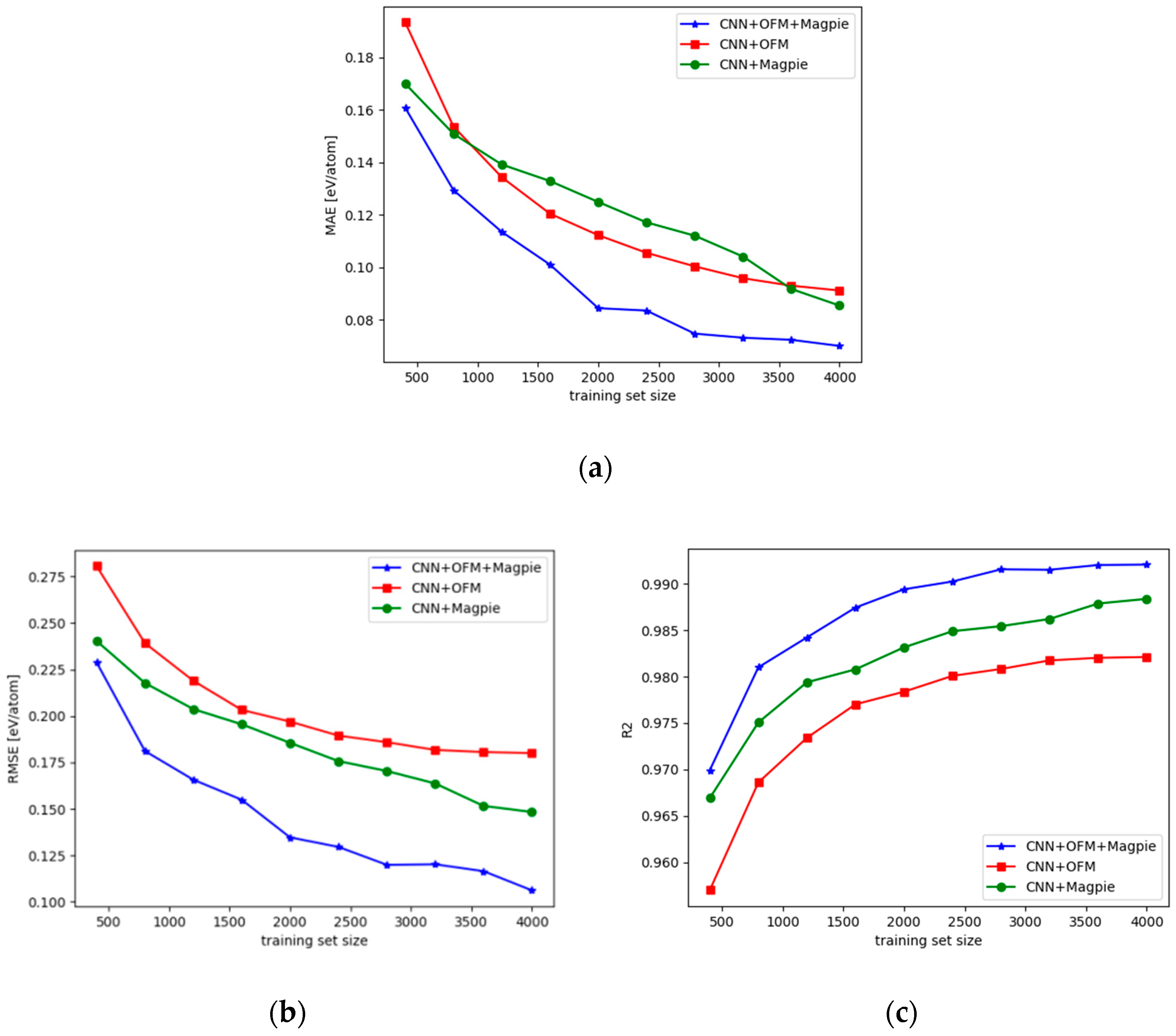
We also compared the performance of the CNN models with hybrid descriptors with those with only one type of features. We found that feature fusion is important to achieve the highest formation energy prediction performance over the tested dataset.
(4)
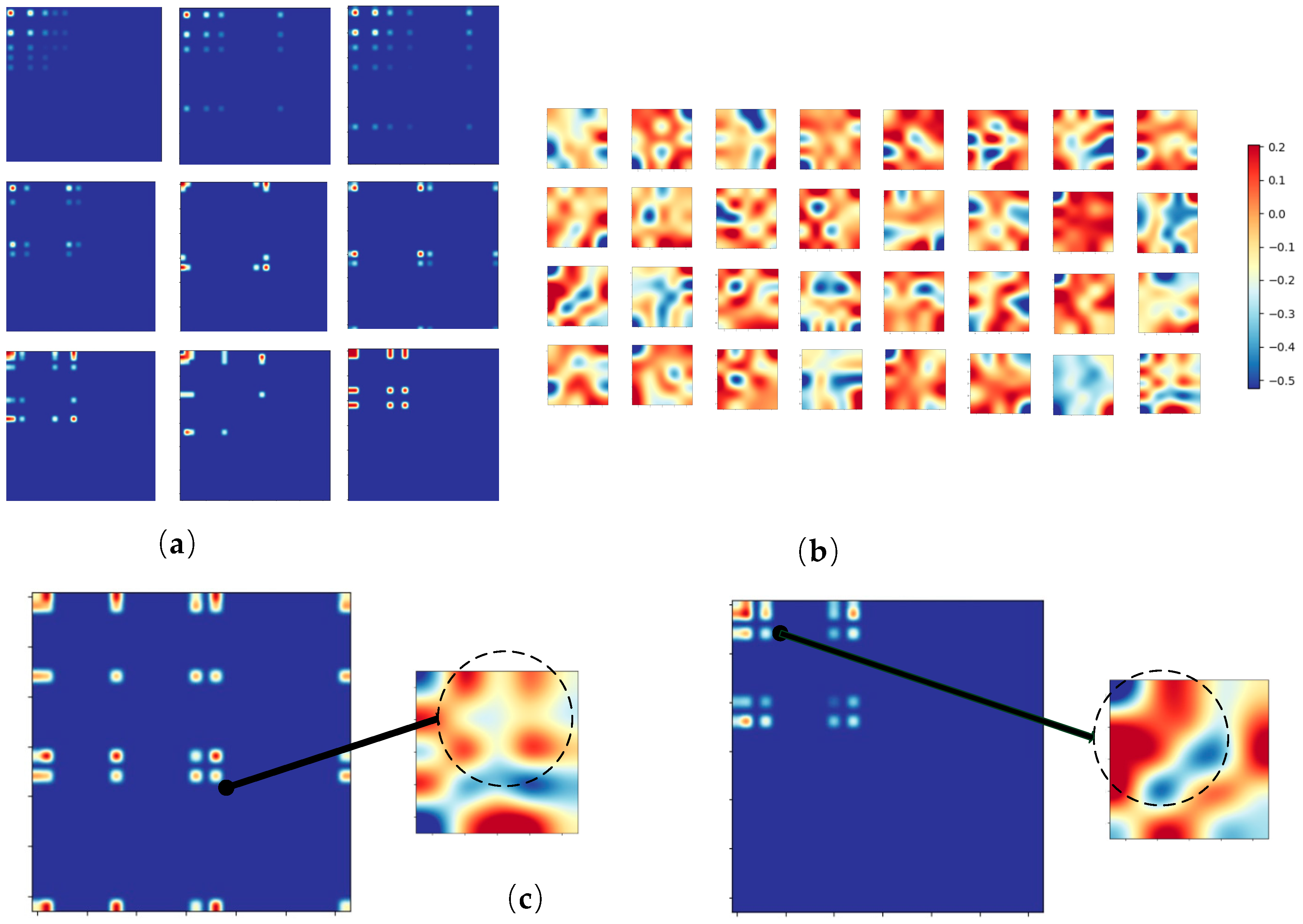
Through visualization of the features extracted by the filters of the learned convolution neural network, interpretable analysis of CNN-OFM is provided.

2. Materials and Methods

Two-dimensional descriptors such as OFM have the benefit of preserving spatial or other structural relations of atoms in materials and thus can better materials properties. While conventional machine learning algorithms usually use one-dimensional vectors as input, we propose to exploit the convolutional neural network models to utilize and mine the spatial relationship of the elements in two-dimensional descriptors such as OFM. We also explore the complementary relationship of the OFM features and the well-known Magpie features.
To evaluate the performances of CNN models with 2D OFM features, we compared it with conventional machine learning algorithms with the one-dimensional OFM vector including feed-forward neural network (FNN), kernel ridge regression (KRR) and support vector regression (SVR). Then, two CNN models with one-dimensional Magpie features and two-dimensional OFM features are fused to create the hybrid CNN models that show the best prediction performance for formation energy prediction.

2.1. Materials Dataset Preparation

When using machine learning algorithms, the selected datasets also have a great impact on the prediction results. In order to make the prediction results comparable, we select the dataset used by the authors in studying the OFM descriptor and also use it to predict the formation energy of the materials. This dataset has 4030 crystal materials including transition metal binary alloys (TT), lanthanide metal and transition metal binary alloys (LAT), lanthanide metal and transition metal binary alloys with a light element (X) compound (LATX).The transition metals from the set of {Sc, Ti, V, Cr, Mn, Fe, Co, Ni, Cu, Zn, Y, Zr, Nb, Mo, Tc, Ru, Rh, Pd, Ag, Cd, Hf, Ta, W, Re, Os, Ir, Pt, Au}, the lanthanides from {La, Ce, Pr, Nd, Pm, Sm, Eu, Gd, Tb, Dy, Ho, Er, Tm, Yb, Lu}, and the X elements from {B, C, N, O} are used. These data including structures and formation energies of each material are all acquired from the Material Projects material database [21] and were collected by using the open-source library of matminer [22].

2.2. Orbital Field Matrix Representation of Materials

The materials representation method used in this paper is slightly different from the original OFM descriptor. OFM descriptor define the set of electron configurations as D = {s1, s2, p1, p2, …, p6, d1, d2, …, d10, f1, f2, …, f14}. Then according to the electron orbital distribution of the atom, the unfilled orbitals are set to 1, and others are set 0 (e.g., the electron configurations of Na is [Ne]3s1, so the one-hot vector of Na can be represented as (1,0,0,…,0), electron configuration of atoms can be found in Table S1, in the Supplementary Materials). So all 47 kinds of atoms are represented as one-dimensional vectors of length 32. Next the local structure of the crystal is characterized by the OFM descriptor, which constructs two-dimensional matrices by using one-dimensional vectors of the central atom, and its neighbor atoms which are directly connected with the central atom by chemical bonds, coordination numbers and distance factors. In this paper, considering the fact that inside the real crystal there is no chemical bond but instead atoms are stacked in space, the atoms within the fixed radius of the central atom at the center of the sphere are regarded as neighbor atoms. In addition, due to the different definitions of the coordination number of crystal structures, coordination numbers were no longer considered in our method and only embedded distances between the central atom and the neighbor atom are used. So the local structure of the central atom in the crystal can be calculated in the following form:
M s = i = 1 n s A s T A i   ×   ζ ( r s i )
MS is the representation of the two-dimensional matrix of 32 × 32 for the atom in position s, ns is the number of neighbor atoms surrounding site s, i is the index of the neighbor atom, A s and A i are the one dimensional vectors of the atom with site s and the neighbor atom with index of i, rsi is the distance between the center atom located in position s and the neighbor atom with an index i, ζ ( r s i ) = 1 / r s i . Finally, the local structure of the crystal is used to characterize the entire structure. Furthermore, since formation energy of the crystal is not proportional to the system size, the descriptor for the entire structure is obtained by averaging the descriptors of the local structures to eliminating the effect of size. The entire structure of the crystal can then be expressed in the following form:
F   =   1 N s s N s M s
F is the entire representation of crystals, Ns is the number of all atoms in a cell of a crystal. After the above three steps, a crystal material can be characterized as a 32 × 32 two-dimensional matrix, and 4030 two-dimensional matrices obtained from the dataset will be used as input data for our convolution neural network model, CNN-OFM. For other baseline machine learning methods, the matrices are just flatted into a 1024 one-dimension vectors. In practice, pymatgen library [23] is used to calculate the material representation, and the data needed to make two-dimensional descriptors are obtained by calculating the material structure information obtained from the Materials Project database.

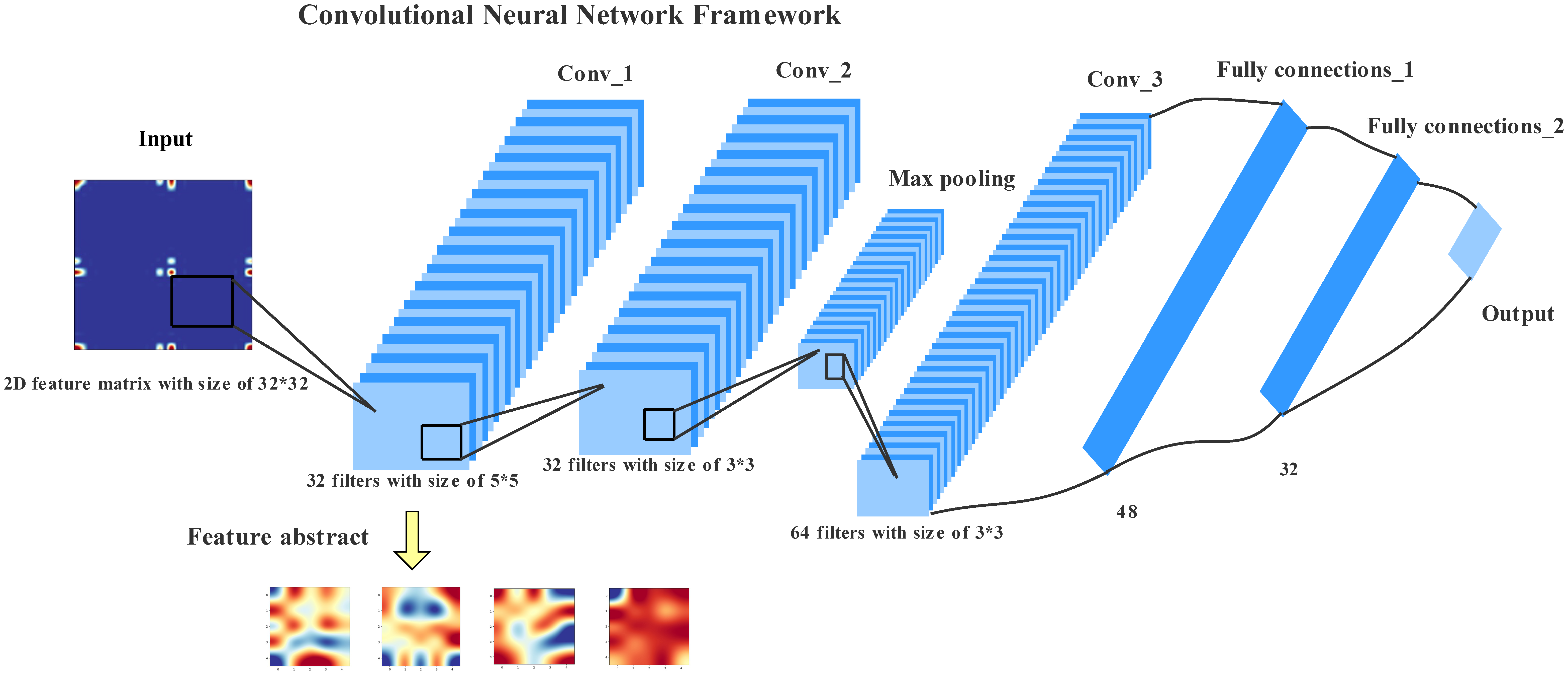
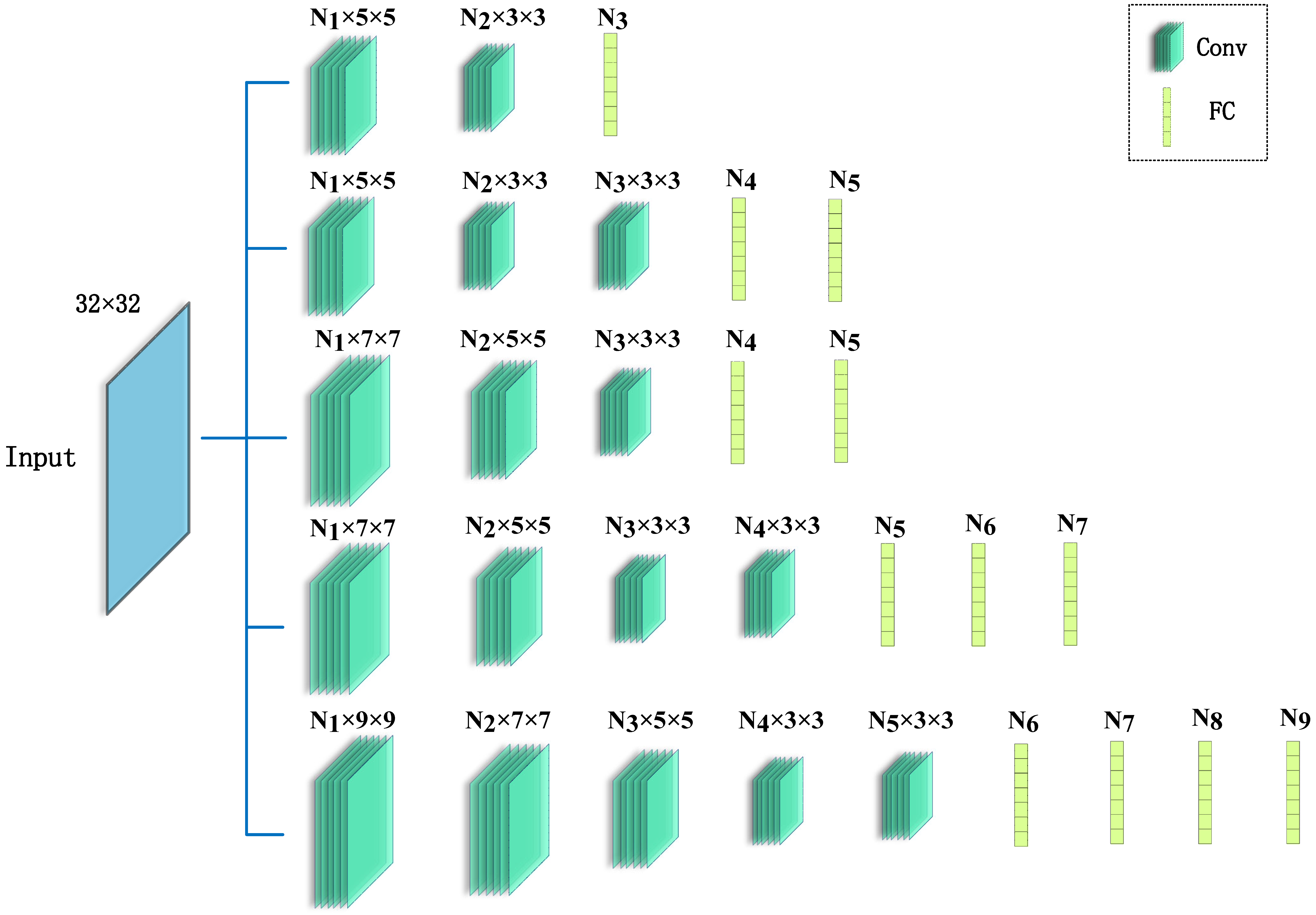
2.3. Convolutional Neural Networks Model

Convolutional neural network (CNN) is one kind of deep learning method characterized for its ability to learn complex features from raw input data. It has achieved superior results across a wide range of application domains with its inherent combination of feature extraction and attribute prediction [24]. Unlike FNN models that have a huge number of trainable parameters for high dimensional input data, the CNN model is faster, more efficient and can identify natural structures by convolution operation. Typical convolutional neural networks consist of multiple, repeating components that are stacked in basic layers: convolution, pooling, fully connected and dropout layer, etc.
Convolution layer employs a convolution operation between the input data and the convolution filters, which improves the algorithm system through the characteristics of sparse interactions, parameter sharing, and equivalent representation. The two-dimensional convolution operation is shown in Equation (3):
( s k ) i , j = ( W k   ×   x ) i , j +   b k
where k = 1, …, K is the index of the feature map and (i, j) is the index of neuron s in the k-th feature map and x represents the input data. Wk and bk are trainable parameters (weights) of linear filters (kernel) and bias for neurons in the k-th feature map respectively. (sk)i,j is the value of the output for the neuron in the k-th feature map with position of (i, j).
Pooling layer can achieve invariance in a small shift of feature maps by maximizing or averaging values in each sub-region of the feature maps. Local invariance is a very useful property, especially when we care about whether a pattern appears and do not care about where it appears.
Fully connected layer is a typical neural network layer where one neuron in the next layer is connected to each neuron in the previous layer by a weight respectively, as shown in Equation (4). The fully connected layer is generally constructed behind the convolutional layer in a convolutional neural network.
y k   =   l W k l x l   +   b k
where yk is the k-th output neuron and Wkl is the weight between xl and yk.
Activation function as part of the convolutional layer and the fully connected layer is used to introduce nonlinear activation operations for the CNN model. It has commonly used activation functions such as ReLU, Sigmoid, etc.
Dropout layer [25] is a method that can increase the generalization of the network architecture by randomly ignoring (dropping) a certain number or proportion of neurons only during the training phase, while also saving training costs.
CNN training also needs to choose the loss function and optimizer. The loss function L is used to calculate the error on the validation dataset during the training process, the optimizer utilize gradient descent [26] and back propagation [26] to propagate the loss function gradient to previous layers. When training a CNN model, the loss will be calculated after each batch size, then according to the loss function gradient δL/δωij, the weight is adapted toward the direction in which the gradient falls with a step size (learning rate) to decrease the loss. Learning rate is a custom parameter and determines the step size for updating the weights in each back-propagation step. The weight update calculation method is as shown in Equation (5):
w i j n e w   =   w i j o l d     η δ L δ w i j
Our convolutional neural network model with two-dimensional OFM matrix for predicting formation energy of materials is shown in Figure 1. The input of the CNN is a 32 × 32 fixed-size two-dimensional matrix. The structure of the CNN model consists of three convolutional layers and two fully connected layers (the pooling layer following the convolutional layer is considered part of the convolutional layer), the output of the last convolutional layer is flattened into a one-dimensional vector for subsequent fully connection layers. Both the convolutional layers and the fully connected layers use ReLU [27] as the activation function, which is simple, fast and can add some sparsity to the network. The output of the network is a continuous numeric value representing the predicted formation energy. Adam [28] optimizer and MAE (Mean Absolute Error) loss function are selected for training the convolutional neural network. Adam optimizer combines the advantages of multiple optimizers and its performance is proved excellent in many applications. Furthermore, we applied 10 times of 10-fold cross-validation in evaluation and employed RMSE, MAE, and R2 to evaluate the performance of CNN-OFM and other baseline machine learning algorithms. The CNN model and the implementation of feature extraction are developed based on the Keras [29] and Tensorflow [30] deep learning libraries.
In addition, to analyze what patterns are extracted by our CNN model to achieve its high performance, we utilized the analysis method commonly used in image pattern recognition for feature extraction. More specifically, the weights of the 32 filters of the first convolutional layer in the CNN model are extracted, visualized, and compared with the input data.

2.4. Regression Algorithms with One-Dimensional Input

To evaluate the performance of CNN-OFM, we also applied several mainstream machine learning algorithms including feedforward neural network (FNN), Support Vector Regression (SVR), and Kernel Ridge Regression (KRR) to the same dataset using one-dimensional OFM features.
Feedforward neural network (FNN) is a classical artificial neural network model for prediction modeling. All neurons in the FNN are hierarchically arranged and each neuron is connected to all neurons in the previous layer with separate weights. It has strong nonlinear mapping ability, but the cost of computing is too large when the number of layers is deep and the number of neurons per layer is high. In this paper, the Adam optimizer and ReLU activation function are used to train the FNN and the Dropout layer is added to avoid overfitting.
Support Vector Regression (SVR) is a powerful regression algorithm that uses the kernel function to map the data from low dimension space to high-dimensional space and then use the support vectors to fit a hyperplane. SVR introduces a soft margin when calculating the loss, which ensures a certain degree of fault tolerance. SVR has excellent performance in prediction problems with high-dimensional features. However, the advantage decreases when the feature size is much larger than the number of samples. The main hyperparameters in SVR include C, gamma, and epsilon. C is penalty parameter of the error term. Gamma is a parameter that comes with the RBF function. It implicitly determines the distribution of data when mapping to a new feature space, the value of the gamma is inversely proportional to the number of support vectors, which will affect the efficiency of training and prediction. Epsilon specifies the epsilon-tube within which no penalty is associated in the training loss function with points predicted within a distance epsilon from the actual value.
Kernel Ridge Regression (KRR) is another machine learning regression method that is widely used in materials property prediction. It combines the kernel method with ridge regression. Both KRR and SVR utilize L2 normalization. But KRR is usually faster than SVR for dataset of medium size. The hyper-parameters in KRR include alpha and gamma, small positive values of alpha improve the conditioning of the problem and reduce the variance of the estimates and gamma is mentioned above. The Random Forest Regression (RF) algorithm is a popular algorithm in real-world application due to its high interpretability ease of construction, and fast running time. It is widely used in statistics, data mining, and machine learning. The hyperparameters in RF are max_features and n_estimators, while max_features is the number of features to consider when looking for the best split, and n_estimators is the number of trees in the forest. All of the above machine learning algorithm models and the 10-fold cross-validation method are implemented using the open-source library Scikit-learn [31].

2.5. Hyperparameters Tuning Strategies

Hyperparameters have a great impact on the predictive performance when applying machine learning algorithms. For example, in SVR, the kernel function determines the feature space of the samples for high-dimensional mapping, and the inappropriate kernel function will result in poor prediction performance. In addition, since there are often multiple hyperparameters for a machine learning algorithm, only adjusting one of them will affect the performance of the model. If one randomly adjusts multiple hyperparameters at the same time, the performance will become uncertain. Therefore, the tuning of hyperparameters can also be regarded as an optimization problem. In recent years, the Bayesian Optimization algorithm [32] has demonstrated outstanding performance in tuning hyperparameters. The Bayesian Optimization algorithm uses prior knowledge to efficiently adjust the hyperparameters and effectively avoids the high computational cost of the exhaustive grid search method hyperparameter tuning. Therefore, the optimization strategy based on Bayesian Optimization algorithm is used here to optimize the hyperparameters.
For CNNs, the number of convolutional layers, the size and number of filters can all be considered hyperparameters, so we have adopted a special strategy for the adjustment of CNN hyperparameters. As shown in Figure 2, we set the number of convolution layers from 2 to 5 layers, while the size of filters and the number of fully connected layers are also gradually increasing, and the number of filters in each convolutional layer and the number of neurons in the fully connected layer (Ni, i = 1, 2, …, 9) are regarded as hyperparameters. For each model structure, the Bayesian Optimization algorithm is used to adjust these hyperparameters. Then, the model with the best prediction performance is selected from multiple structures and the value of each parameter is obtained. Finally, Pooling and The Dropout layer is fine-tuned to determine the final model structure, as shown in Figure 1, while the parameters of the CNN are also shown in the figure. The CNN for magpie has three convolution layers and two fully connected layers, while the specific structure is mentioned in Tables S2 and S3. Similarly, we set the number of layers of the FNN from 2 to 6, taking the number of neurons in each layer as the hyperparameters, and adjust them with the Bayesian Optimization algorithm. For the OFM descriptor, the optimal model has 5 layers, and the number of neurons in each layer is 344, 177, 344, 177, 177. For the Magpie descriptor, the optimal model layer is 6 layers, and each layer of neurons is 177, 344, 177, 344, 177, 177. For conventional machine learning algorithms such as SVR, KRR, RF, we directly adjust the relevant hyperparameters. For the OFM descriptor, SVR: C = 100, epsilon = 10−6, gamma = 1. KRR: alpha = 45.98, gamma = 84.14. RF: n_estimators = 879, max_features = 105. For Magpie descriptor, SVR: C = 1000, epsilon = 10−6, gamma = 10−7, KRR: alpha = 0.2428, gamma = 855.5, RF: n_estimators = 500, max_ features = 28. The Bayesian Optimization algorithm is implemented using the Sherpa library [33].

3. Results and Discussions

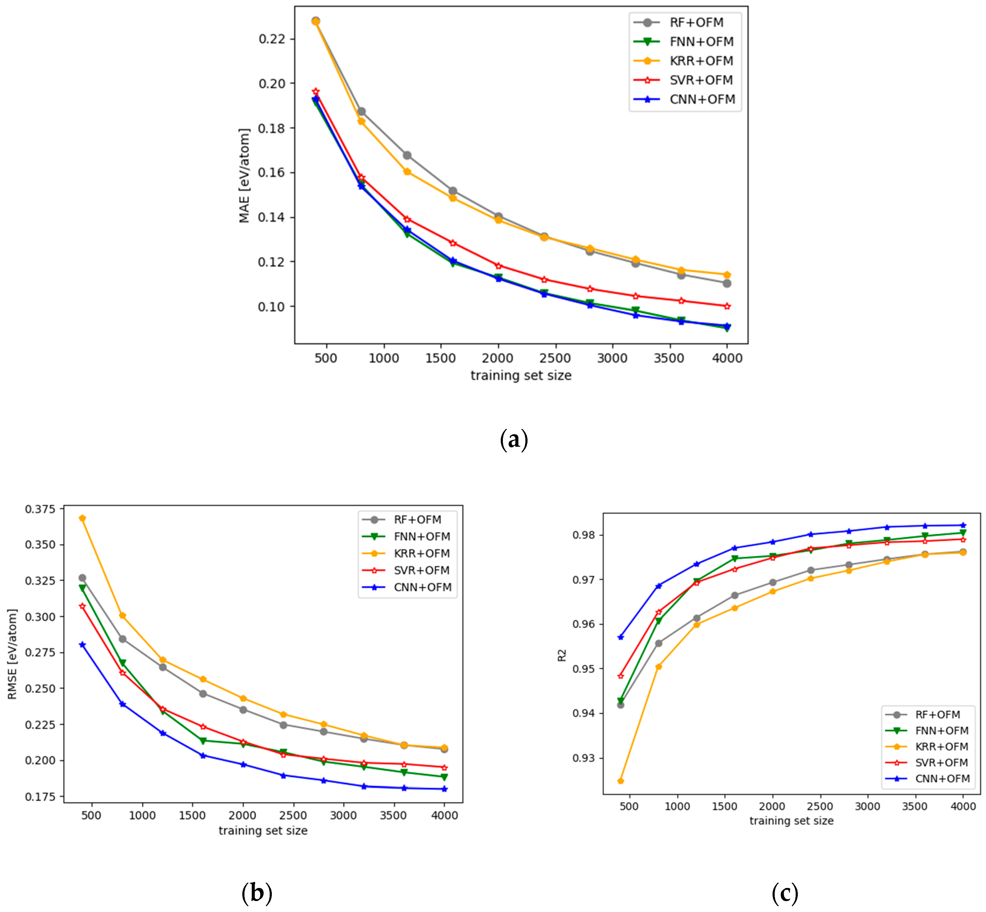
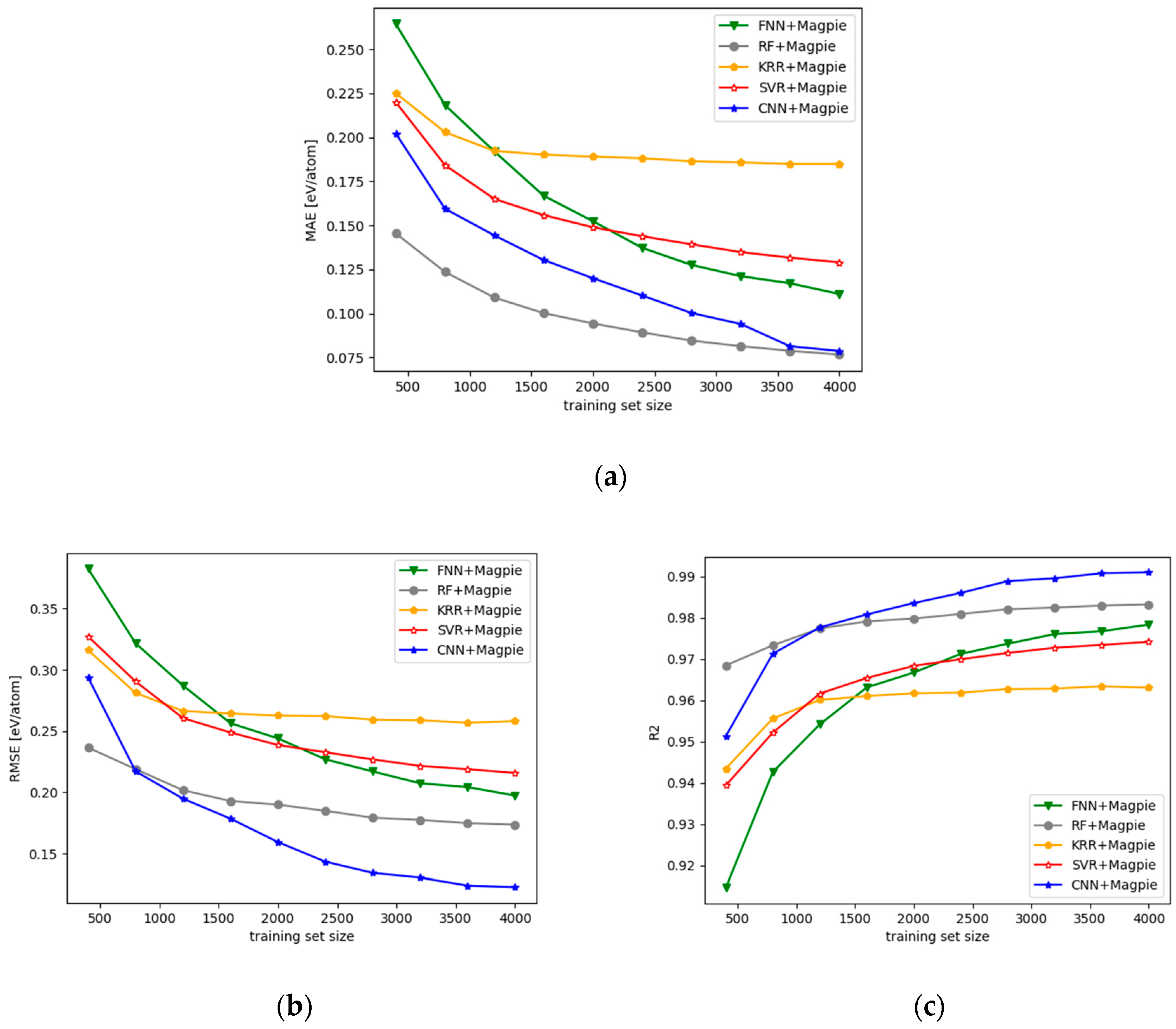
3.1. Performance of the CNN Models with 2D OFM Features

First, we compared the performances of the convolutional neural networks using 2D OFM descriptors as raw features and various machine learning methods using the one-dimensional flatten OFM features. In order to obtain stable results, each algorithm was evaluated using 10-fold cross-validations ten times. Figure 3 shows the RMSE, MAE and R2 values of all models using different numbers of samples. It shows that the performance of the CNN model is significantly better than those of other ML models, and the performances of the five compared models are ranked as CNN > FNN > SVR > KRR > RF. Comparison of all prediction models is further shown in Table 1 when the number of samples is set as 4000. The CNN model obtained a cross-validated RMSE of 0.18 eV/atom, a cross-validated MAE of 0.0911 eV/atom, and an R2 value of 0.9821. All three values are better than those of other prediction models (the designers of the OFM descriptor use the KRR model for prediction, and our CNN’s result is better than their results). This result shows that our CNN model has excellent prediction performance by using two-dimensional OFM features as input due to its capability to exploit the structural information of the orbits for all the atoms of the crystal structures and extract higher level features for effective formation energy prediction compared to one-dimensional vectors.
Next, we compared how the CNN model compares with various ML models with Magpie descriptor. Here, Random Forest (RF), FNN, and KRR all use one-dimensional Magpie features, and the CNN model uses a two-dimensional matrix which was restructured with a magpie feature (We extend the length of one-dimensional magpie descriptor to 144 with zero, then restructured it to a two-dimensional matrix with size of 12 × 12). As shown in Figure 4, Only RF is similar to CNN in terms of MAE errors. For other cases, the performance of our CNN model is still the best. A more detailed performance comparison is shown in Table 2. Among the baseline models, the MAE of RF is as small as that of the CNN, which achieves the best RMSE and R2. The KRR model is the worst for all criteria. The performances of the five compared models are ranked as CNN > RF > FNN > SVR > KRR. The performances of the CNN and several regression methods are depicted in Figure S1 (In the Supplementary Materials). It is worth noting that the simple and fast DT model achieved a performance comparable with the more advanced machine learning models of FNN and KRR. Actually, Ahneman et al. [34] utilized an algorithm based on Random Forest to achieve good performance in material property prediction.
The above two experiments compared the performances of various ML prediction models using flatten one-dimensional descriptors and CNN using two-dimensional descriptor. Among all the models, the CNN model achieved the best results using two-dimensional OFM descriptor or two-dimensional magpie descriptor. This demonstrates the potential of CNNs in formation energy prediction using two-dimensional descriptors. This is possibly because the CNN model with its hierarchical feature extraction capability can better utilize the characteristics of the two-dimensional descriptor than other machine learning models.
It is interesting that OFM descriptors and Magpie features use totally different information from the materials while both can be used to achieve good prediction performance in formation energy prediction (Table 1 and Table 2). Since each type of descriptors has certain limitations in representing materials, it is thus desirable to exploit the complementary information of multiple descriptors to get improved prediction performance. So we propose a deep learning model that combines two descriptor types for material property prediction. As shown in Figure 5, this deep learning model performs convolution operations on each of the two types of descriptors for feature extraction. The extracted high-level features are then flattened and concatenated/fused as an input of the subsequent fully connected network for material property prediction. In the previous two experiments, we obtained two CNNs with the best performances when using the OFM descriptors and the Magpie descriptors. We can utilize the parameters of these two CNNs as a reference for setting the parameters of the multiple-descriptor CNN, which can be found in Table S4.
We applied the CNN with hybrid descriptors to predict the formation energy of the afore-mentioned dataset with the results shown in Figure 6. It is observed that the performance of the multiple-descriptor CNN is consistently better than the performance of CNNs using either one kind of descriptors, which indicates that multiple-descriptor CNNs can use complementary characteristics of both descriptors to improve the prediction accuracy of material properties. RMSE, MAE and R2 in the three cases with a sample size of 4000 are listed in Table 3. We found that the results of the multiple-descriptor CNN have been significantly improved: RMSE, MAE and R2 are all the best. This experiment confirms that the combination of descriptors can have great potential in materials property prediction. We also found that there are algorithms such as SchNet [35] that can achieve better formation energy prediction performance than ours when the number of samples of their dataset is 60,000. However, on a smaller subset with 3000 training examples, SchNet just achieves an MAE of 0.127 eV/atom, and our multiple-descriptor CNN model can achieves an MAE of 0.07 eV/atom on 4000 training examples, which is comparable or better than theirs when using a small data set.

3.2. Analysis over the Features Extracted by the CNN Model

In order to acquire understanding how the CNN model works in terms of feature extraction from the raw OFM input, we visualized and analyzed the patterns learned by the CNN. Firstly, we visualized two-dimensional OFM descriptors which describe the distribution of atomic electron orbital interactions in different materials (Figure 7a). It is observed that the transformed two-dimensional descriptor has several characteristics: (1) the matrices are relatively sparse and data in the upper left corner of the matrix is in general denser than other locations; (2) the matrices have a certain symmetry along the leading diagonal; (3) data in the matrices spread from the upper left to the lower right. The sparsity of the data in the 2D matrices and thus the flatten 1024 one-dimensional vectors may have caused the relatively lower performance of the convention machine learning algorithms as we have evaluated.
To further analyze how the CNN model learns, we visualized the features as shown in Figure 7. The 32 filters of the first convolutional layer in the trained CNN model are extracted and visualized as shown in Figure 7b. The filters have a size of 5 × 5. To contrast with the input matrices (OFM descriptor), as shown in Figure 7c, the distribution patterns of the data in the input matrices can be identified, such as the form of square point, wavy distribution, and etc., all of which can be observed visually. These patterns potentially reflect the distribution of electrons in the material, and the recognition of the pattern can effectively grasp the influence of the electronic distribution on the target property, and these patterns can be used in a reverse design of materials.

4. Conclusions

Instead of relying on feature engineering, this paper proposes convolutional neural network models for materials formation energy prediction using the electron configurations and Magpie features. The performances of the CNN model using two-dimensional OFM descriptors are compared to those of various machine learning algorithms using a flattened one-dimensional OFM descriptor for prediction of materials formation energy with extensive experiments on the dataset of 4030 crystal materials. The results showed that the performance of CNN models is better than all other baseline algorithms, including SVM, KRR, RF and FNN.
To further demonstrate the power of the proposed CNN algorithm, we compared the CNN with 2D reshaped Magpie features with machine learning algorithms based on the 136-feature one-dimensional Magpie descriptors over the same dataset. Experimental results showed that our CNN model with two-dimensional feature restructured with Magpie descriptors still outperforms all other baseline machine algorithms with one-dimensional Magpie features. This shows the advantage of CNN models in feature extraction for materials property prediction.
Finally, we propose a multiple-descriptor hybrid CNN model, CNN-OFM-Magpie which fuses a CNN with OFM descriptors and a CNN with Magpie descriptors with greatly improved prediction performance. This indicates that the combination of descriptors can exploit the complementary information of different descriptors. Finally, we visualized and analyzed the generated two-dimensional matrices, extracted the filters of the first convolutional layer in the trained CNN model and contrasted it with the original two-dimensional matrix, which showed that some patterns in original matrices can be identified. Overall, our study shows that CNN models with two-dimensional descriptors can effectively utilize the information of features and improve the performance of predictive models, which provides a new perspective for using multi-dimensional material descriptors.

Supplementary Materials

The following are available online at https://www.mdpi.com/2073-4352/9/4/191/s1, Table S1: Electron configuration of atoms used in data set, Table S2: Architectures of CNN for OFM descriptor, Table S3: Architectures of CNN for Magpie descriptor, Figure S1: Scatter plots and error metrics for CNN and several regression methods.

Author Contributions

Conceptualization, Z.C., J.H.; methodology, Z.C. and J.H.; software, Z.C. and Y.D.; validation, Z.C., X.L. and J.H.; investigation, Z.C., Y.D., Z.X. and J.H.; resources J.H.; writing—original draft preparation, Z.C., C.N. and J.H.; writing—review and editing, Z.C., J.H., Z.X.; supervision, J.H. and S.Q.; project administration J.H.; funding acquisition J.H.

Funding

This research was funded by The National Natural Science Foundation of China under Grant No. 51741101; Z.X. is partially supported by the National Science Foundation EPSCoR Program under NSF Award # OIA-1655740. Any Opinions, findings and conclusions or recommendations expressed in this material are those of the author(s) and do not necessarily reflect those of the National Science Foundation.

Acknowledgments

We gratefully acknowledge the support of NVIDIA Corporation with the donation of the Titan X Pascal GPU used for this research and the support of National Institute of Measurement and Testing Technology with providing the semi-anechoic laboratory.

Conflicts of Interest

The authors declare no conflict of interest.

References

  1. Takahashi, K.; Tanaka, Y. Materials informatics: A journey towards material design and synthesis. Dalton Trans. 2016, 45, 1497–1499. [Google Scholar] [CrossRef]
  2. Butler, K.T.; Davies, D.W.; Cartwright, H.; Isayev, O.; Walsh, A. Machine learning for molecular and materials science. Nature 2018, 559, 547–555. [Google Scholar] [CrossRef] [PubMed]
  3. Li, Y.; Liu, L.; Chen, W.; An, L. Materials genome: Research progress, challenges and outlook. Sci. Sin. Chim. 2018, 48, 243–255. [Google Scholar] [CrossRef]
  4. Ramprasad, R.; Batra, R.; Pilania, G.; Mannodi-Kanakkithodi, A.; Kim, C. Machine learning in materials informatics: Recent applications and prospects. NPJ Comput. Mater. 2017, 3, 54. [Google Scholar] [CrossRef]
  5. Ward, L.; Wolverton, C. Atomistic calculations and materials informatics: A review. Curr. Opin. Solid State Mat. Sci. 2017, 21, 167–176. [Google Scholar] [CrossRef]
  6. Meredig, B.; Agrawal, A.; Kirklin, S.; Saal, J.E.; Doak, J.W.; Thompson, A.; Zhang, K.; Choudhary, A.; Wolverton, C. Combinatorial screening for new materials in unconstrained composition space with machine learning. Phys. Rev. B 2014, 89, 0941049. [Google Scholar] [CrossRef]
  7. Seko, A.; Togo, A.; Tanaka, I. Descriptors for Machine Learning of Materials Data. In Nanoinformatics; Tanaka, I., Ed.; Springer: Singapore, 2018. [Google Scholar]
  8. Swann, E.; Sun, B.; Cleland, D.M.; Barnard, A.S. Representing molecular and materials data for unsupervised machine learning. Mol. Simul. 2018, 44, 905–920. [Google Scholar] [CrossRef]
  9. Ghiringhelli, L.M.; Vybiral, J.; Levchenko, S.V.; Draxl, C.; Scheffler, M. Big Data of Materials Science: Critical Role of the Descriptor. Phys. Rev. Lett. 2015, 114, 105503. [Google Scholar] [CrossRef]
  10. Ziletti, A.; Kumar, D.; Scheffler, M.; Ghiringhelli, L.M. Insightful classification of crystal structures using deep learning. Nat. Commun. 2018, 9, 2775. [Google Scholar] [CrossRef]
  11. Calfa, B.A.; Kitchin, J.R. Property Prediction of Crystalline Solids from Composition and Crystal Structure. Aiche J. 2016, 62, 2605–2613. [Google Scholar] [CrossRef]
  12. Ward, L.; Agrawal, A.; Choudhary, A.; Wolverton, C. A general-purpose machine learning framework for predicting properties of inorganic materials. NPJ Comput. Mater. 2016, 2, 16028. [Google Scholar] [CrossRef]
  13. Faber, F.; Lindmaa, A.; Von Lilienfeld, O.A.; Armiento, R. Crystal structure representations for machine learning models of formation energies. Int. J. Quantum Chem. 2015, 115, 1094–1101. [Google Scholar] [CrossRef]
  14. Tien, L.P.; Kino, H.; Terakura, K.; Miyake, T.; Tsuda, K.; Takigawa, I.; Hieu, C.D. Machine learning reveals orbital interaction in materials. Sci. Technol. Adv. Mater. 2017, 18, 756–765. [Google Scholar]
  15. Zhou, Q.; Tang, P.; Liu, S.; Pan, J.; Yan, Q.; Zhang, S. Learning atoms for materials discovery. PNAS 2018, 115, E6411–E6417. [Google Scholar] [CrossRef] [PubMed]
  16. Hansen, K.; Montavon, G.; Biegler, F.; Fazli, S.; Rupp, M.; Scheffler, M.; von Lilienfeld, O.A.; Tkatchenko, A.; Müller, K. Assessment and Validation of Machine Learning Methods for Predicting Molecular Atomization Energies. J. Chem. Theory Comput. 2013, 9, 3404–3419. [Google Scholar] [CrossRef]
  17. Kajita, S.; Ohba, N.; Jinnouchi, R.; Asahi, R. A Universal 3D Voxel Descriptor for Solid-State Material Informatics with Deep Convolutional Neural Networks. Sci. Rep. 2017, 7, 16991. [Google Scholar] [CrossRef]
  18. De, S.; Bartok, A.P.; Csanyi, G.; Ceriotti, M. Comparing molecules and solids across structural and alchemical space. Phys. Chem. Chem. Phys. 2016, 18, 13754–13769. [Google Scholar] [CrossRef]
  19. Cecen, A.; Dai, H.; Yabansu, Y.C.; Kalidindi, S.R.; Song, L. Material structure-property linkages using three-dimensional convolutional neural networks. Acta Mater. 2018, 146, 76–84. [Google Scholar] [CrossRef]
  20. Xie, T.; Grossman, J.C. Crystal Graph Convolutional Neural Networks for an Accurate and Interpretable Prediction of Material Properties. Phys. Rev. Lett. 2018, 120, 145301. [Google Scholar] [CrossRef] [PubMed]
  21. Jain, A.; Shyue, P.O.; Hautier, G.; Chen, W.; Richards, W.D.; Dacek, S.; Cholia, S.; Gunter, D.; Skinner, D.; Ceder, G.; et al. Commentary: The Materials Project: A materials genome approach to accelerating materials innovation. APL Mater. 2013, 1, 0110021. [Google Scholar] [CrossRef]
  22. Ward, L.; Dunn, A.; Faghaninia, A.; Zimmermann, N.E.R.; Bajaj, S.; Wang, Q.; Montoya, J.; Chen, J.; Bystrom, K.; Dylla, M.; et al. Matminer: An open source toolkit for materials data mining. Comput. Mater. Sci. 2018, 152, 60–69. [Google Scholar] [CrossRef]
  23. Ong, S.P.; Richards, W.D.; Jain, A.; Hautier, G.; Kocher, M.; Cholia, S.; Gunter, D.; Chevrier, V.L.; Persson, K.A.; Ceder, G. Python Materials Genomics (pymatgen): A robust, open-source python library for materials analysis. Comput. Mater. Sci. 2013, 68, 314–319. [Google Scholar] [CrossRef]
  24. Azimi, S.M.; Britz, D.; Engstler, M.; Fritz, M.; Mücklich, F. Advanced Steel Microstructural Classification by Deep Learning Methods. Sci. Rep. 2018, 8, 2128. [Google Scholar] [CrossRef]
  25. Srivastava, R.K.; Greff, K.; Schmidhuber, J. Training Very Deep Networks. 2015. Eprint arXiv:1507.06228. Available online: https://arxiv.org/pdf/1507.06228.pdf (accessed on 9 March 2019).
  26. Lecun, Y.; Bottou, L.; Bengio, Y.; Haffner, P. Gradient-based learning applied to document recognition. Proc. IEEE 1998, 86, 2278–2324. [Google Scholar] [CrossRef]
  27. Glorot, X.; Bordes, A.; Bengio, Y. Deep sparse rectifier neural networks. In Proceedings of the 14th International Conference on Artificial Intelligence and Statistics, Ft. Lauderdale, FL, USA, 11–13 April 2011; pp. 315–323. [Google Scholar]
  28. Kingma, D.; Ba, J. Adam: A Method for Stochastic Optimization. In Proceedings of the 3rd International Conference for Learning Representations, San Diego, CA, USA, 7–9 May 2015. [Google Scholar]
  29. Chollet, F. Keras. 2015. Available online: https://keras.io (accessed on 9 March 2019).
  30. Abadi, M.; Agarwal, A.; Barham, P.; Brevdo, E.; Chen, Z.; Citro, C.; Corrado, G.S.; Davis, A.; Dean, J.; Devin, M.; et al. TensorFlow: Large-Scale Machine Learning on Heterogeneous Distributed Systems. 2016. Available online: https://www.tensorflow.org (accessed on 9 March 2019).
  31. Pedregosa, F.; Varoquaux, G.E.; Gramfort, A.; Michel, V.; Thirion, B.; Grisel, O.; Blondel, M.; Prettenhofer, P.; Weiss, R.; Dubourg, V.; et al. Scikit-learn: Machine Learning in Python. J. Mach. Learn. Res. 2011, 12, 2825–2830. [Google Scholar]
  32. Shahriari, B.; Swersky, K.; Wang, Z.; Adams, R.P.; de Freitas, N. Taking the Human Out of the Loop: A Review of Bayesian Optimization. Proc. IEEE 2016, 104, 148–175. [Google Scholar] [CrossRef]
  33. Hertel, L.; Collado, J.; Sadowski, P.; Baldi, P. Sherpa: Hyperparameter Optimization for Machine Learning Models. In Proceedings of the 32nd Conference on Neural Information Processing Systems, Montreal, QC, Canada, 3–8 December 2018. [Google Scholar]
  34. Ahneman, D.T.; Estrada, J.G.; Lin, S.; Dreher, S.D.; Doyle, A.G. Predicting reaction performance in C–N cross-coupling using machine learning. Science 2018, 360, 186–190. [Google Scholar] [CrossRef]
  35. Schütt, K.T.; Sauceda, H.E.; Kindermans, P.J.; Tkatchenko, A.; Müller, K.R. SchNet—A deep learning architecture for molecules and materials. J. Chem. Phys. 2017, 148, 241722. [Google Scholar] [CrossRef] [PubMed]
Figure 1. Convolutional neural network for material property prediction using Orbital-field matrix descriptors and feature extraction.
Crystals 09 00191 g001
Figure 2. The hyper-parameters of the CNN involving convolutional layers, fully connected layers, number and size of filters.
Crystals 09 00191 g002
Figure 3. Prediction performances of different models using OFM features. (a) MAE of different training set size. (b) RMSE of different training set size. (c) R2 of different training set size.
Crystals 09 00191 g003
Figure 4. Prediction performance of different models using Magpie descriptors. (a) MAE of different training set size. (b) RMSE of different training set size. (c) R2 of different training set size.
Crystals 09 00191 g004
Figure 5. Architecture of the hybrid convolutional neural network with multiple descriptors.
Crystals 09 00191 g005
Figure 6. Prediction performance of multiple descriptor CNN when using OFM and Magpie descriptor. (a) MAE of different training set size. (b) RMSE of different training set size. (c) R2 of different training set size.
Crystals 09 00191 g006
Figure 7. Feature extraction and analysis. The color in the figures indicates the value of points, as shown in the color bar. (a) visualization of two-dimensional OFM descriptors; (b) visualization of filters of the first convolutional layer; (c) the relation of the CNN filters and original two-dimensional OFM matrices.
Crystals 09 00191 g007
Table 1. RMSE (eV/atom), MAE (eV/atom) and R2 values of cross-validation results of all prediction models using the OFM descriptor.
Regression ModelRMSEMAER2
SVR0.19500.10000.9790
KRR0.20540.11740.9767
RF0.20750.11030.9762
FNN0.19410.10370.9791
CNN0.18000.09110.9821
Table 2. RMSE (eV/atom), MAE (eV/atom) and R2 values of cross-validation results for each prediction model using Magpie descriptors.
Regression ModelRMSEMAER2
SVR0.21580.12900.9741
KRR0.25800.18490.9630
RF0.17360.07780.9832
FNN0.19730.11100.9783
CNN0.12270.07860.9910
Table 3. RMSE (eV/atom), MAE (eV/atom) and R2 values of cross-validation results in three cases of CNN.
DescriptorRMSEMAER2
OFM0.18000.09110.9821
Magpie0.12270.07860.9910
OFM + Magpie0.10620.07000.9920

