Abstract
We numerically study surface models defined on hexagonal disks with a free boundary. 2D surface models for planar surfaces have recently attracted interest due to the engineering applications of functional materials such as graphene and its composite with polymers. These 2D composite meta-materials are strongly influenced by external stimuli such as thermal fluctuations if they are sufficiently thin. For this reason, it is very interesting to study the shape stability/instability of thin 2D materials against thermal fluctuations. In this paper, we study three types of surface models including Landau-Ginzburg (LG) and Helfirch-Polyakov models defined on triangulated hexagonal disks using the parallel tempering Monte Carlo simulation technique. We find that the planar surfaces undergo a first-order transition between the smooth and crumpled phases in the LG model and continuous transitions in the other two models. The first-order transition is relatively weak compared to the transition on spherical surfaces already reported. The continuous nature of the transition is consistent with the reported results, although the transitions are stronger than that of the reported ones.
1. Introduction
The two-dimensional surface model proposed by Helfrich is a model for biological membranes composed of lipid molecules, and it shares almost the same mathematical structure with the Polyakov’s rigid string model for elementary particles in subatomic scales [1,2]. In those models, the extrinsic curvature or bending energy plays an essential role in maintaining the smooth shape of surfaces, and because of its mathematical transparency, many studies have been conducted on the phase structure of the model between the smooth and crumpled phases [3,4,5,6,7,8,9]. The discrete surface models defined on triangulated lattices have also been extensively studied by Monte Carlo (MC) simulations [10,11,12,13,14,15,16,17,18,19].
However, the order of the crumpling transition is still controversial. Since the discrete model depends on the discretization of continuous Hamiltonian, we have a variety of discrete models [20,21]. Indeed, the curvature energy itself has a lot of variation such as extrinsic and intrinsic curvatures. For almost all of these discrete models, MC studies predict that the models undergo a first-order crumpling transition if the lattice is of spherical topology and allowed to self-intersect (⇔ self-intersecting) [20]. Here, we should note that only self-intersecting and fixed-connectivity lattice models are studied in this paper, and self-avoiding models and fluid surface models are not considered [15,16]. Intrinsic curvature models also have a first-order crumpling transition even on a disk surface [21], and the intrinsic curvature models are also out of consideration in this paper. The first-order crumpling transition is supported by theoretical studies on the basis of non-perturbative renormalization group techniques [8,9]. In contrast, it is reported that the order of transition is of second-order on the free boundary lattices [22,23]. Therefore, this continuous transition combining the above-mentioned first-order one indicates that the order of transition depends on the surface topology; either spheres or free boundary planar disks.
In this paper, we study three different surface models by the parallel tempering MC (PTMC) technique to check whether or not the transition is of second-order on triangulated disks with a free boundary. The PTMC technique was developed to simulate the spin glass models at very low temperature, where the standard Metropolis MC technique is not effective [24,25]. It is also reported that this PTMC technique can be applied to phenomena which undergo first-order transitions [26,27]. Therefore, we expect that the PTMC technique can also be used to study the phase structure of the surface models in this paper even if these models have first-order transitions [28].
We should here comment on the reason why the crumpling transition is of interest. Indeed, graphite oxide sheets in solvents have a crumpled state [29,30]. Crumpled states can also be observed in graphenes [31,32]. The surface condition of graphenes is altered by corrugations, and therefore ripples, wrinkles and crumples emerge [33,34]. These surface states modify or enhance the material properties such as mechanical, electrical and optical ones [35]. The crumpled graphene, for example, is expected to have enhanced chemical activities and energy storage capacities [36]. In addition to pure graphenes, polymer-graphene nano-composite or graphene-based polymers (or polymer-based graphenes) also has the crumpled states [37,38,39,40]. For the application of crumpled states of these graphene-based materials, it is interesting to study their stability against thermal fluctuation or some other stimuli in environmental conditions [41]. Therefore, the crumpled state is worthwhile studying in terms of phase transition.
This paper is organized as follows: In Section 2, the three different models and the PTMC technique are described in detail. Readers who are familiar with or not interested in these topics can skip Section 2 and go to Section 3, where the simulation results including snapshots of surfaces are presented. In Section 4, we summarize the results and comment on the future study.
2. Models and Monte Carlo Technique
2.1. Triangulated Disk
Discrete surface models are defined on such a triangulated disk shown in Figure 1. The lattice is characterized by the numbers , which are the total number of vertices, the total number of edges, and the total number of triangles. Using the number L of division of the hexagon edge, we have the expressions for these numbers such that . The lattice shown in Figure 1 is obtained by , and hence . We chose a sufficiently small L to visualize the lattice structure. The lattices used in the simulations are larger than the lattice in Figure 1. The lattice spacing a for the edge length can be used as the length scale [42]. However, the simulation data are not directly compared to the experimental ones in this paper, and for this reason we fix a to for simplicity.
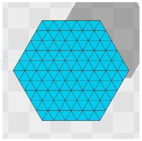
Figure 1.
A hexagonal lattice discretized by regular triangles. The total number of vertices N including those on the boundary is given by . This number is calculated by the formula , where is the number of division of the edge of the original hexagon. This type of hexagonal lattice is used to define discrete Hamiltonians of the surface models studied in this paper.
2.2. Landau-Ginzburg surface Model
The so-called Landau-Ginzburg surface model is first introduced and studied by Paczuski, Kardar and Nelson in [43], and this model is also numerically studied in [44]. Let be the surface position. The continuous Hamiltonian is given by
where is a tangential vector along the local coordinate axis on the surface and plays a role of the order parameter. The real numbers are the coefficients of the energy terms, which are square and quadratic with respect to . The second term is defined by the square of second-order differentials .
The continuous energy in Equation (1) can be written more explicitly such that
The detailed information on the role of each term is written in Ref. [44], and we briefly describe the outline of each term. The first term is given by the integration of length squares of the tangential vectors, and it simply plays a role of the tensile energy. The second term plays a role of the bending energy and the in-plane shear energy, and the third term contains both the tensile and the shear energy components. The final term is a quadratic tensile energy term.
The discrete Hamiltonian is as follows [44]:
We briefly summarize how to obtain the discrete Hamiltonian in Equation (3) from the continuous one in Equation (2). First of all, we note that the local coordinate origin of the triangle 123 in Figure 2a is at the vertex 1, and hence the differentials and in of Equation (2) are replaced by
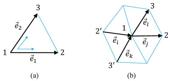
Figure 2.
(a) A local coordinate on a triangle 123 and the edge vectors and along the coordinates axes and . A local coordinate for the discretization of the second-order differential in of LG model on (b) a vertex of coordination number (hexagonal).
Recalling that there are two other local coordinate origins on the triangle 123, and including all possible terms for the differentials and and with the factor , we have
where is not written in Figure 2a. The integration is replaced by the sum over triangles such that . By replacing the summation convention from the sum over triangles to the sum over bonds , we have in Equation (3). We should note that this energy is also defined on the triangles of the boundary.
The second order derivative such as in is replaced by using the vectors and on the hexagon in Figure 2b, because and are considered as the discretization of along the coordinate axis corresponding to the local coordinate axis at the vertex 1. Another diagonal line on this hexagon is considered as the axis, and thereby the square of Laplacian is replaced by using the vectors , , and in Figure 2b. Thus, we have in Equation (3) as a discrete bending energy corresponding to the continuous one in Equation (3). The reason for the factor in the discrete expression is that every vertex inside the boundary is assumed to be the center of hexagon, and therefore the summation is triply duplicated. Strictly speaking, the duplication at the vertices close to the boundary is not triple, however, the coefficient is not so important and is simply fixed to , which is the same as in the spherical model [44]. In the discrete , denotes the sum over the three different diagonal lines, and denotes the sum over the corresponding local coordinates on the hexagon.
Please note that on the hexagonal lattice, such as shown in Figure 1, the coordination number at the vertices inside the boundary is given by , where the coordination number is the total number of bonds emanating from the vertex i. This is in sharp contrast to spherical lattices, which must include the vertices with . Therefore, the vertex with in Figure 2b is sufficient for the discretization of for all internal vertices. On the boundary vertices, the definition of energy is slightly different from that on the internal vertices. On the vertices with , the square of Laplacian is simply replaced by instead of . Moreover, the bending energy is not defined on the vertices with on the boundary (see Figure 1).
In the continuous and of Equation (2), the derivatives and are replaced by and in Equation (4) on the triangle in Figure 2a. The discretization technique is exactly the same as the one assumed in , and hence we have the discrete energies and in Equation (3).
The partition function Z is given by the multiple integrations of the vertex positions such that
where the prime in denotes that the center of the mass of surface is fixed at the origin of .
From the scale invariance of Z, we have
where is defined by [7,44]. This relation in Equation (7) can be used to check whether the simulation is correctly performed or not.
2.3. Canonical Model
We start with the continuous form of Hamiltonian of the canonical model, which is defined by a mapping from a two-dimensional surface M to the three-dimensional Euclidean space , such that
The variable , which is originally used to denote the surface position in , is now used for the symbol of the mapping. Another variable denoted by g in is the metric function on M, where is a matrix. The metric originally is not a variable but is determined by a local coordinate, which is fixed arbitrarily by hand from the reparametrization invariance. This invariance is a symmetry of the model under 2D coordinate transformations on the surface in . Thus, the model is slightly extended from the original one in the sense that is a variable that should be physically determined. As a consequence, we have the possibility to obtain surfaces which cannot be in in the extended model, whether this is meaningful or not. For example, let us consider the metric
on a surface discretized by piece-wise linear triangles such as in Figure 3a, where is not always identical to between the edge vectors and [45]. If for all triangles, then this metric is identical with the discrete induced metric . However, if the angles do not satisfy the triangle equality, i.e., the sum of three internal angles is not always equal to , then the surface with such metric in Equation (9) generally cannot be realized in .
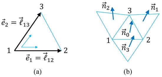
Figure 3.
Lattice structure for discretization of the canonical surface model. (a) A local coordinate on the triangle 123 with the edge vectors and , and (b) the triangle 123 and its three nearest-neighbor triangles, where the normal vector interacts with . The local coordinate in (a) is exactly the same as that in Figure 2a.
The continuous Hamiltonian is given by
where the surface tension coefficient is always fixed to . The symbol denotes the inverse of , and g is its determinant. We should note that assumed in the expression of in Equation (10) is a variable that should be determined just like the mapping as mentioned above [46]. Note also that this Hamiltonian is a two-dimensional extension of the polymer model of Doi-Edwards [47].
Here, we should note that the real surface in corresponding to the material under consideration is described by the induced metric . This allows us to consider that the surface with a given metric is different from the real surface, pointing to the possibility for the surface to correspond to this . Therefore, from this set of surfaces, a physically meaningful surface should be uniquely determined by the modeling. For this reason, we introduce a two-dimensional surface M in addition to the real surface with , both of which should be physically determined. This is another extension of the surface model, and this is the meaning of the mapping described in Equation (8). Please note that the surface M is not necessarily a manifold [45,48,49].
The problem is then how to determine for M. One possible and simple technique is to fix to the Euclidean metric such that . In this case, M is a simple two-dimensional Euclidean space and plays no role in describing the model, however, we use M to express the domain in the two-dimensional integrations in . Thus, the only variable to be determined is , and is now given by
One simple reason for why we assume the Euclidean metric for is as follows: The Hamiltonian in Equation (10) is invariant under an arbitrary conformal transformation with a positive function on M. This invariance is described by and implies that the metric can be chosen relatively freely, and therefore it is fixed to the simplest one such that .
The discrete Hamiltonians are obtained from the continuous one in Equation (11) by the replacement of the differentials in Equation (4). Here, we use the symbols and for the edge vectors (Figure 3a), and for the edge (or bond) length. Thus, we obtain
where the factor is eliminated from both and for simplicity. This is exactly the same as of the LG model in Equation (3) up to the numerical factor. The symbol in denotes the sum over all bonds connecting the vertices i and j. In contrast, in the sum of denotes the triangles sharing a common bond (Figure 3b), and the unit normal vector is defined on the triangle i. The partition function of the canonical model is exactly the same as Z in Equation (6) for the LG model except the Hamiltonian in the Boltzmann factor.
2.4. Modified Canonical Model
The third model, which we call “modified canonical model”, is obtained from the same continuous Hamiltonian in Equation (11) assumed for the canonical model. The only difference is a discretization of the bending energy , where the unit normal vector at the vertex i (Figure 4a) is used as well as the normal vector on the triangle i (Figure 3b). The discrete Hamiltonian is given by [20]
where in is the unit normal vector of the triangle connected to the vertex i. The normal vector at the vertex i is defined by (Figure 4a)
where is the area of the triangle . Please note that the interaction range of the normal vectors is slightly larger than that of the canonical model (Figure 4b). In fact, only two nearest neighbor vectors and are directly coupled in in Equation (12) of the canonical model, and as a consequence only three nearest neighbor vectors are coupled to (see Figure 3b). In contrast, as shown in Figure 4b, the non-nearest neighbor and , of which the triangles i and j do not directly contact each other, are coupled to in in Equation (13) of the modified model.
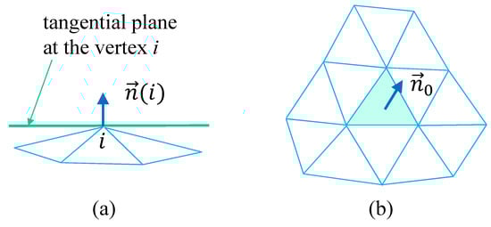
Figure 4.
Lattice structure for discretization of the modified canonical surface model. (a) The tangential plane at the vertex i and its normal vector , and (b) a triangle and its neighboring triangles, where the normal vector interacts with those of the neighboring triangles. The range of interaction is slightly larger than that shown in Figure 3b.
2.5. Parallel Tempering Monte Carlo Technique
The so-called parallel tempering Monte Carlo (PTMC) technique developed for the spin glass model at low temperatures is successfully applied to the first-order crumpling transition of the canonical model on spherical lattices [28]. In this subsection, the outline of the PTMC technique applied to the tethered surface model is briefly presented.
Let represent a system of configuration with a given , which is assumed to be changed. In the case of the LG model, the parameter is also changed while the other three parameters are fixed in the simulations in this paper. In this PTMC, replicas are simulated in parallel by the standard Metropolis MC (MMC) simulation technique [50,51], and the systems are exchanged after sufficiently long MMC runs. Because of this exchange, the total number of different combinations is .
The replicas are updated as follows:
- (P1)
- Perform long MMC simulations for replicas
- (P2)
- Exchange all nearest neighbor systems and with the probability
- (P3)
- Repeat and
We should note that the process can be performed in parallel as mentioned above. In the exchange process , only bending energy is used, and no information on the other energy is used in the canonical and modified canonical models. This is also true for the LG model, and no information on the energies , and is left out in the exchange process.
Figure 5a,b intuitively show the difference of MMC and PTMC simulations for four replica systems. The numbers denote the bending rigidities such as , and the color blocks denote the configurations . The combination of is exchanged as the iterations evolve in the PTMC simulation.
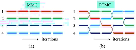
Figure 5.
Illustration of how the replica systems evolve in (a) MMC and (b) PTMC simulations. In (a) MMC simulations, each system evolves independent of the other systems, while in (b) PTMC simulations, the systems are exchanged.
Here, we briefly show that all micro states satisfy the canonical Boltzmann distribution as a result of PTMC simulations. Let be a probability distribution for all the states such that
where is independent of and given by for the LG model and for the other two models. The in Equation (16) is the Boltzmann distribution function of the state . If the PTMC exchange satisfies the detailed balance condition described by
then we understand from the well-known uniqueness theorem that this P is the uniquely determined probability [28]. Please note that the right-hand side of Equation (17) is obtained from the left-hand side by exchanging and . Thus, we should prove that in Equation (16) satisfies the condition in Equation (17). This can be accomplished in two steps. The first step is to see that Equation (17) for in Equation (16) is equivalent with the relation
under the condition given by Equation (15). The second step is to see that the relation in Equation (18) is correct. This second step is almost trivial from the definitions of and in Equation (15). The first step is also straightforward to prove.
The assumed parameters for the simulations including the total number of MC sweeps (MCS) are listed in Table 1, where 1 MCS consists of the processes and of PTMC. In Table 1, the symbol N is the total number of vertices, #total (MCS) and #therm (MCS) are the total number of MCS and the total number of thermalization MCS, and denotes the number of iterations performed in per 1 MC sweep. This is fixed to (or ), and this implies that the total number of MMC (including thermalization) iterations for each replica is 10 (or 20) times larger than the #total (MCS). The is the total number of replicas, and and () are the bending rigidity of the replica 1 and , is the difference of between two neighboring replicas, which will be exchanged in the process . The total number of iterations #total for the large lattices in the latter two models is not so large compared to those for smaller lattice in the LG model.

Table 1.
The parameters assumed for the simulations; denotes the total number of MMC iterations performed in the process per 1 MCS for each replica, and () are the bending rigidity of the replica 1 and , and is the difference of between two neighboring replicas.
3. Simulation Results
3.1. Snapshots
Firstly, in the presentation section, we show snapshots, which are obtained as one of the configurations from the replicas and in each model. In the upper (lower) low in Figure 6, the snapshots are obtained from the replica () of the (a) LG, (b) canonical, and (c) modified canonical models. The size of lattices are the largest for these snapshots, and hence from Table 1 all are given by . From Table 1, we find that the values of corresponding to these replicas are given as follows: (a) (upper), (lower), (b) (upper), (lower), and (c) (upper), (lower). In the LG model simulations, the parameters are fixed to
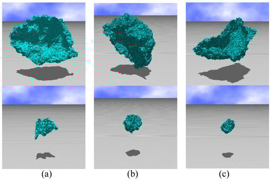
Figure 6.
Snapshots of surfaces obtained in the replica such that in the upper low and in the lower low, which correspond to the flat phase and the crumpled phase, respectively, in each model. The models and lattice size N are (a) the LG model, , (b) the canonical model, N = 44,287, and (c) the modified canonical model, N = 20,917.
We find that the surfaces in the upper low are globally bending but almost flat while those in the lower low shrink to a small ball. From this observation, we understand that the surfaces in the upper and lower lows are in the flat and crumpled phases, respectively, in all of the models.
3.2. Bending Energy and Mean Square Gyration
The bending energy of the LG model is calculated only on the internal vertices, because the definition of on the boundary vertices is slightly different from that on the internal vertices as described in Section 2.2. In Figure 7a–i, we plot the bending energy of the LG model and the other models, the specific heat
and the peak of the specific heat. We should note that is the total number of internal bonds for the LG model, where is the total number of internal vertices and hence is the total number of the diagonal lines such as in Figure 2b. The reason why this is used for in the LG model is because the first term of in Equation (3) is defined on such diagonal lines, and the second term is also defined on a pair of diagonal lines and in Figure 2b, and there are three different such diagonal lines on each internal vertex. For the other two models, is the total number of internal bonds, on which the bending energy is defined, where is the total number of edges given in Section 2.1. Please note that in Equation (24) for the LG model is defined also by using N. The curves of in Figure 7h for the modified model are fluctuating, and this fluctuation may be due to the fact that the total number of iterations is not sufficient for this model as mentioned above, though reasonable peak values are obtained.
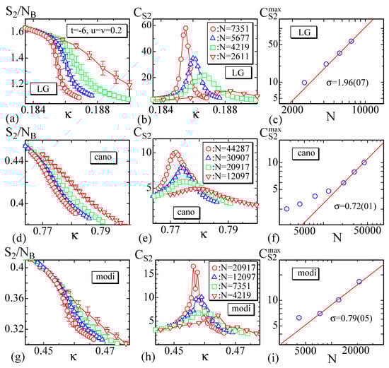
Figure 7.
The bending energy per bond , the specific heat , and the log-log plot of the peak value vs. N for (a–c) the LG model, (d–f) the canonical model, and (g–i) the modified canonical model.
From the LG model data plotted in Figure 7a–c, we see that the abruptly changes against , and correspondingly the has the anomalous peak showing the existence of the crumpling transition. As mentioned above, the parameters are fixed to the values in Equation (19) and remain unchanged. The peak heights vs. N are plotted in log-log scale in Figure 7c, where N is used. The data obtained by the other models are also plotted in Figure 7d–i. Fitting the largest three data of to the scaling relation
we have
We find from these results that the transition of the LG model is of the first order while in the other two models the transition is of second-order, because in the LG model and in the other models. We note that should be for the first order transitions, because is expected to scale as , where L is the linear size of the lattice [52]. However, the present result is almost twice of this expectation and indicates that the dimension D of lattice is effectively . One possible reason is that the surface is self-intersecting, and hence, the total number or density of possible configurations is larger than that in the case of . The first result in Equation (22) of the LG model is qualitatively comparable to of the canonical model on spherical lattice in Ref. [28], because both results indicate that the transition is of first-order. In contrast, the latter two results in Equation (22) of the other models indicate a second-order transition, and hence these two are completely different from the result in Ref. [28]. We consider that this difference simply stems from the difference in the lattice topology or structure; sphere and disk, which are surfaces without a boundary and with a free boundary, or are compact and non-compact.
We calculate the coefficient in Equation (21) for the LG model using the specific heat of the bending energy in Equation (12), and we have , which is almost identical to the first result in Equation (22). This indicates that the results in Equation (22) for the LG model is reliable, although this result is obtained from the bending energy on the internal vertices only.
The problem here is ascertaining why the result of LG model in Equation (22) is different from the others. Firstly, we should be reminded that it is predicted that the LG model has a continuous crumpling or wrinkling transition from the mean filed analysis [11]. However, as mentioned in Ref. [28], the basic assumption for the mean field analysis that the surface fluctuation is relatively small is not always true even for the models. This is considered to be why the result of the LG model deviates from the mean field prediction and has the first-order transition even on the lattice with a free boundary. Next, we have to consider where the difference comes from in the order of transitions between the LG model and the other two models. One possible origin is the shear stress or resistance to shear deformation expected in the LG model; it is not expected in the other models. The bending energy assumed in the LG models is identical to in the other models up to a numerical factor, and this has no shear resistance to in-plane deformation of triangles; it has only a resistance to the bending or out-of-plane deformation. Thus, the only source for the shear resistance is the Gaussian bond potential in the two models, while in the LG model, and as well as have resistance to shear stresses. Here, we should note that all models are fixed-connectivity or tethered models, and the shear resistance is not negligible compared to the fluid surface models on dynamically triangulated lattices. In the tethered models, any deformations of triangles except simple expansion/shrinkage accompany a shear resistance, because all triangles tend to become regular in the equilibrium configurations. Please note that the simple expansion and shrinkage of triangles are suppressed because the mean bond length remains constant due to the scale invariant-property of the partition function.
The mean square radius of gyration defined by
its variance
and the peak values are plotted in Figure 8a–i. The fluctuations of the data in Figure 8h are relatively large due to the same reason for mentioned above. We also find that rapidly changes, where has a peak . The peak position on the axis for of the LG model is almost identical with the position for , while those for and in the other models are considerably different from each other. This difference is not observed in the canonical model on spherical lattice in Ref. [28], where a first-order transition is expected and where the transition point is very clear and detected uniquely even by numerical simulations. In contrast, continuous transitions are relatively unclear in general, and hence the transition points of the latter two models are relatively hard to observe. Moreover, the total number of iterations for these are not always sufficiently large as mentioned above. These are possible reasons for the deviation of the transition points observed in and .
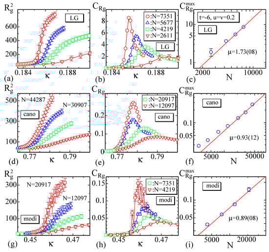
Figure 8.
The mean square gyration , its variance , and the log-log plot of the peak value vs. N for (a–c) the LG model, (d–f) the canonical model, and (g–i) the modified canonical model.
The peak values are expected to scale according to
By fitting the largest three data of in Figure 8c,f,i to this relation, we have
These results also support the proposition that the LG model has a first-order transition and the other models a second-order transition, though the coefficient of the canonical model is close to and the transition is close to a first-order one. The reason why in Equation (26) of the LG model is may be the fact that the surface is not self-avoiding [28]. We should note that the order of transition depends on its definition. If we call a transition first-order only if the coefficient for the variance of Hamiltonian is , then the canonical and modified models clearly have a second-order transition from the results in Equation (22). In general, the coefficient for the bending energy is more important than as a coefficient for the determination of the order of transition. Thus, it is reasonable to consider that the crumpling transitions of the canonical and modified canonical models are continuous transitions.
3.3. Binder Quantity and Fractal Dimension
Firstly. in this subsection, we calculate the Binder quantity defined by [53,54]
for the LG model (Figure 9a). It is expected that has a peak and at the first-order transition point. To see whether this expectation is satisfied or not, vs. are plotted in Figure 9b, where the Binder quantity for is also plotted. The solid lines are also drawn by Mathematica command “Interpolation” for the data of and . The value on the vertical axis expected from the extrapolations is almost identical with , while is slightly smaller than . This deviation of seems due to the size effect, because the lattice size is not so large compared to those used in Ref. [28], where and are observed.
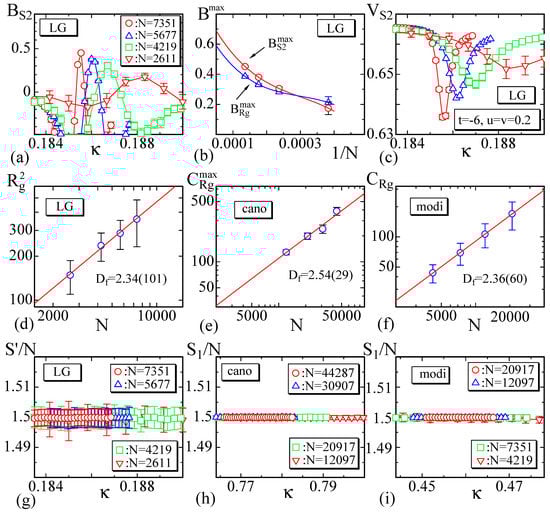
Figure 9.
(a) The Binder quantity , (b) the peak values and vs with solid lines drawn by Mathematica command “Interpolation”, and (c) the Binder cumulant for the LG model. The log-log plot of vs. N of (d) the LG model, (e) the canonical model, and (f) the modified canonical model. of (g) the LG model, and of (h) the canonical model and (i) the modified canonical model.
A first-order transition is also reflected in the Binder cumulant , which is defined by [53,54]
The Binder cumulant for is also defined analogously to Equation (28). These quantities are expected to have the minimum and at the first-order transition point, and this expectation is confirmed in Figure 9c, where only is plotted. It is also found that the position of on the axis is almost the same as that of in Figure 7b. This also implies that reflects the first-order transition.
In the other two models, the quantities and (and those for ) are unclear compared to the case of LG model. One of the reasons for this is the continuous nature of the transition; the convergent speed of the simulation is very slow close to the transition point.
Next, we calculate the fractal dimension , which is defined by
To calculate this quantity at the transition point, we plot vs. N in Figure 9d–f in the log-log scale, where are obtained at the peak position of in Figure 8b,e,h. By fitting the plotted data to Equation (29), we obtain
Since the errors of are large in the first and third models (see Figure 9d,f), the errors in are also relatively large. The values of within these errors are comparable to at the first-order transition point of the canonical model on the spherical lattice in Ref. [28].
To check the simulations are performed correctly, we can use the relations
where of the first one is given in Equation (7), and . The second equality is also obtained by using almost the same technique for the first one. The symbol is omitted for these and for simplicity. The results plotted in Figure 9g–i are consistent with these predictions in Equation (31).
4. Summary and Conclusions
In this paper, we study the crumpling transition of a planar surface with a free boundary by parallel tempering Monte Carlo (PTMC) simulations using three different tethered lattice models; the Landau-Ginzburg (LG) model, the canonical (cano) model, and the modified canonical (modi) model, defined on triangulated fixed-connectivity lattices of disk topology. The order of the transition is first order in the LG model, while it is of second order in the other models. This second-order nature of the transition is consistent with the result reported in [22,23].
The models studied in this paper are not self-avoiding, however, the transition between the crumpled and smooth phases indicates that these states are stable against thermal fluctuations. This can give insights into studies on real materials such as graphene, where the crumpled states are expected to have many technological applications.
In the presence of impurity, a new phase is expected to appear, and the surface critical exponents are also expected to change from those of the model without impurity [55]. Thus, it is of great interest to study the planar surface model with impurities.
Author Contributions
A.S. performed planning and modeling and evaluated the simulation results; H.K. performed planning, modeling and simulations and wrote the paper.
Acknowledgments
The author H.K. acknowledges D. Mouhanna and J.P. Kownacki for discussions. This work is supported in part by JSPS KAKENHI Grant Number JP17K05149.
Conflicts of Interest
The authors declare no conflict of interest.
Abbreviations
The following abbreviations are used in this manuscript:
| MC | Monte Carlo |
| PTMC | parallel tempering Monte Carlo |
| MMC | Metropolis Monte Carlo |
| MCS | Three letter acronym |
| LG | Landau Ginzburg |
| cano | canonical |
| modi | modified canonical |
References
- Helfrich, W. Elastic Properties of Lipid Bilayers: Theory and Possible Experiments. Z. Naturforsch C 1973, 28, 693–703. [Google Scholar] [CrossRef] [PubMed]
- Polyakov, A.M. Fine structure of strings. Nucl. Phys. B 1986, 268, 406–412. [Google Scholar] [CrossRef]
- Peliti, L.; Leibler, S. Effects of Thermal Fluctuations on Systems with Small Surface Tension. Phys. Rev. Lett. 1985, 54, 1690–1693. [Google Scholar] [CrossRef] [PubMed]
- Guitter, E.; David, F.; Leibler, S.; Peliti, L. Crumpling and Buckling Transitions in Polymerized Membranes. Phys. Rev. Lett. 1988, 61, 2949–2952. [Google Scholar] [CrossRef]
- David, F.; Guitter, E. Crumpling Transition in Elastic Membranes: Renormalization Group Treatment. Europhys. Lett. 1988, 5, 709–714. [Google Scholar] [CrossRef]
- Nelson, D. The Statistical Mechanics of Membranes and Interfaces. In Statistical Mechanics of Membranes and Surfaces, 2nd ed.; Nelson, D., Piran, T., Weinberg, S., Eds.; World Scientific: Singapore, 2004; pp. 1–17. [Google Scholar]
- Wheater, J.F. Random surfaces: From polymer membranes to strings. J. Phys. A Math. Gen. 1994, 27, 3323–3354. [Google Scholar] [CrossRef]
- Kownacki, J.-P.; Mouhanna, D. Crumpling transition and flat phase of polymerized phantom membranes. Phys. Rev. E 2009, 79, 040101. [Google Scholar] [CrossRef]
- Essafi, K.; Kownacki, J.P.; Mouhanna, D. First-order phase transitions in polymerized phantom membranes. Phys. Rev. E 2014, 89, 042101. [Google Scholar] [CrossRef]
- Bowick, M.; Travesset, A. The statistical mechanics of membranes. Phys. Rep. 2001, 344, 255–308. [Google Scholar] [CrossRef]
- Bowick, M.J. Fixed-connectivity Membranes. In Statistical Mechanics of Membranes and Surfaces, 2nd ed.; Nelson, D., Piran, T., Weinberg, S., Eds.; World Scientific: Singapore, 2004; pp. 323–357. [Google Scholar]
- Gompper, G.; Kroll, D.M. Triangulated-surface Models of Fluctuating Membranes. In Statistical Mechanics of Membranes and Surfaces, 2nd ed.; Nelson, D., Piran, T., Weinberg, S., Eds.; World Scientific: Singapore, 2004; pp. 59–426. [Google Scholar]
- Kantor, Y.; Karder, M.; Nelson, D.R. Tethered surfaces: Statics and dynamics. Phys. Rev. A 1987, 35, 3056–3071. [Google Scholar] [CrossRef]
- Kantor, Y.; Nelson, D.R. Phase Transitions in Flexible Polymeric Surfaces. Phys. Rev. A 1987, 36, 4020–4032. [Google Scholar] [CrossRef]
- Ho, J.-S.; Baumga¨rtner, A. Simulations of Fluid Self-Avoiding Membranes. Europhys. Lett. 1990, 12, 295–300. [Google Scholar] [CrossRef]
- Ambjo¨rn, J.; Irba¨ck, A.; Jurkiewicz, J.; Petersson, B. The theory of dynamical random surfaces with extrinsic curvature. Nucl. Phys. B 1993, 393, 571–600. [Google Scholar] [CrossRef]
- Kownacki, J.-P.; Diep, H.T. First-order transition of tethered membranes in three-dimensional space. Phys. Rev. E 2002, 66, 066105. [Google Scholar] [CrossRef] [PubMed]
- Nishiyama, Y. Crumpling transition of the triangular lattice without open edges: Effect of a modified folding rule. Phys. Rev. E 2010, 81, 041116. [Google Scholar] [CrossRef] [PubMed]
- Nishiyama, Y. Crumpling transition of the discrete planar folding in the negative-bending-rigidity regime. Phys. Rev. E 2010, 82, 012102. [Google Scholar] [CrossRef]
- Endo, I.; Koibuchi, H. First-order phase transition of the tethered membrane model on spherical surfaces. Nucl. Phys. B 2006, 732, 426–443. [Google Scholar] [CrossRef]
- Igawa, M.; Koibuchi, H.; Yamada, M. Monte Carlo simulations of a tethered membrane model on a disk with intrinsic curvature. Phys. Lett. A 2005, 338, 433–438. [Google Scholar] [CrossRef]
- Bowick, M.J.; Catterall, S.M.; Falcioni, M.; Thorleifsson, G.; Anagnostopoulos, K.N. The Flat Phase of Crystalline Membranes. J. Phys. I 1996, 6, 1321–1345. [Google Scholar] [CrossRef]
- Cuerno, R.; Caballero, R.G.; Gordillo-Guerrero, A.; Monroy, P.; Ruiz-Lorenzo, J.J. Universal behavior of crystalline membranes: Crumpling transition and Poisson ratio of the flat phase. Phys. Rev. E 2016, 93, 022111. [Google Scholar] [CrossRef]
- Hukushima, K.; Nemoto, K. Exchange Monte Carlo method and application to spin glass simulations. J. Phys. Soc. Jpn. 1996, 65, 1604–1608. [Google Scholar] [CrossRef]
- Takayama, H.; Hukushima, K. Computational experiment on glassy dynamic nature of field-cooled magnetization in ising spin-glass model. J. Phys. Soc. Jpn. 2007, 76, 013702. [Google Scholar] [CrossRef]
- Neuhaus, T.; Magiera, M.P.; Hansmann, U.H.E. Efficient parallel tempering for first-order phase transitions. Phys. Rev. E 2007, 76, 045701R. [Google Scholar] [CrossRef] [PubMed]
- Fiore, C.E. First-order phase transitions: A study through the parallel tempering method. Phys. Rev. E 2008, 78, 041109. [Google Scholar] [CrossRef] [PubMed]
- Usui, S.; Koibuchi, H. Parallel TemperingMonte Carlo Simulations of Spherical Fixed-Connectivity Model for Polymerized Membranes. J. Stat. Phys. 2016, 162, 701–711. [Google Scholar] [CrossRef]
- Koltonow, A.R.; Luo, C.; Luo, J.; Huang, J. Graphene Oxide Sheets in Solvents: To Crumple or Not to Crumple? ACS Omega 2017, 2, 8005–8009. [Google Scholar] [CrossRef]
- Shang, J.; Chen, Y.; Zhou, Y.; Liu, L.; Wang, G.; Li, X.; Kuang, J.; Liu, Q.; Dai, Z.; Miao, H.; et al. Effect of folded and crumpled morphologies of graphene oxide platelets on the mechanical performances of polymer nanocomposites. Polymer 2014, 68, 131–139. [Google Scholar] [CrossRef]
- Novoselov, K.S.; Geim, A.K.; Morozov, S.V.; Jiang, D.; Zhang, Y.; Dubonos, S.V.; Grigorieva, I.V.; Firsov, A.A. Electric Field Effect in Atomically Thin Carbon Films. Science 2004, 306, 666–669. [Google Scholar] [CrossRef] [PubMed]
- Novoselov, K.S.; Jiang, D.; Schedin, F.; Booth, T.J.; Khotkevich, V.V.; Morozov, S.V.; Geim, A.K. Two-dimensional atomic crystals. Proc. Natl. Acad. Sci. USA 2005, 102, 10451–10453. [Google Scholar] [CrossRef] [PubMed]
- Deng, S.; Berry, V. Wrinkled, rippled and crumpled graphene: An overview of formation mechanism, electronic properties, and applications. Mater. Today 2016, 19, 197–212. [Google Scholar] [CrossRef]
- Papageorgiou, D.G.; Kinloch, I.A.; Young, R.J. Mechanical properties of graphene and graphene-based nanocomposites. Prog. Mat. Sci. 2017, 90, 75–127. [Google Scholar] [CrossRef]
- Zang, J.; Ryu, S.; Pugno, N.; Wang, Q.; Tu, Q.; Buehler, M.J.; Zhao, X. Multifunctionality and control of the crumpling and unfolding of large-area graphene. Nat. Mat. 2013. [Google Scholar] [CrossRef] [PubMed]
- Luo, J.; Jang, H.D.; Sun, T.; Xiao, L.; He, Z.; Katsoulidis, A.P.; Kanatzidis, M.G.; Gibson, J.M.; Huang, J. Compression and Aggregation-Resistant Particles of Crumpled Soft Sheets. ACS Nano 2011, 5, 8943–8949. [Google Scholar] [CrossRef] [PubMed]
- Chee, W.K.; Lim, H.N.; Huang, N.M.; Harrison, I. Nanocomposites of Graphene/ Polymers: A Review. RSC Adv. 2015, 5, 68014–68051. [Google Scholar] [CrossRef]
- Di´ez-Pascual, A.M.; Sa´nchez, J.A.L.; Capilla, R.P.; Di´az, P.G. Recent Developments in Graphene/Polymer Nanocomposites for pplication in Polymer Solar Cells. Polymers 2018, 10, 217. [Google Scholar] [CrossRef]
- Kim, H.; Abdala, A.A.; Macosko, C.W. Graphene/Polymer Nanocomposites. Macromolecules 2010, 43, 6515–6530. [Google Scholar] [CrossRef]
- Dai, Z.; Weng, C.; Liu, L.; Hou, Y.; Zhao, X.; Kuang, J.; Shi, J.; Wei, Y.; Lou, J.; Zhang, Z. Multifunctional Polymer-Based Graphene Foams with Buckled Structure and Negative Poisson’s Ratio. Sci. Rep. 2016, 6, 32989. [Google Scholar] [CrossRef] [PubMed]
- Marsden, A.J.; Papageorgiou, D.G.; Valle´s, C.; Liscio, A.; V Palermo, V.; Bisse, M.A.; Young, R.J.; Kinloch, I.A. Electrical percolation in graphene-polymer composites. 2D Mater. 2018, 5, 032003. [Google Scholar] [CrossRef]
- Creutz, M. Quarks, Gluons and Lattices; Cambridge University Press: Cambridge, UK, 1983. [Google Scholar]
- Paczuski, M.; Kardar, M.; Nelson, D.R. Landau Theory of the Crumpling Transition. Phys. Rev. Lett. 1988, 60, 2638–2640. [Google Scholar] [CrossRef] [PubMed]
- Koibuchi, H.; Shobukhov, A. Monte Carlo simulations of Landau-Ginzburg model for membranes. Int. J. Mod. Phys. C 2014, 25, 1450033. [Google Scholar] [CrossRef]
- Koibuchi, H. Monte Carlo studies of triangulated spherical surfaces in the two-dimensional space. Nucl. Phys. B 2010, 836, 186–203. [Google Scholar] [CrossRef]
- Ueno, K. Algebraic geometry and string theory. In Developments in Mathematical Physics. Developments in Mathematical Physics 1988, 111–149. (In Japanese) [Google Scholar]
- Doi, M.; Edwards, S.F. The Theory of Polymer Dynamics; Oxford University Press: Oxford, UK, 1986. [Google Scholar]
- Koibuchi, H.; Sekino, H. Monte Carlo studies of a Finsler geometric surface model. Physica A 2014, 393, 37–50. [Google Scholar] [CrossRef]
- Proutorov, E.; Matsuyama, N.; Koibuchi, H. Finsler geometry modeling and Monte Carlo study of liquid crystal elastomer under electric fields. J. Phys. Condens. Matter. 2018, 30, 405101. [Google Scholar] [CrossRef] [PubMed]
- Metropolis, N.; Rosenbluth, A.W.; Rosenbluth, M.N.; Teller, A.H. Equation of State Calculations by Fast Computing Machines. J. Chem. Phys. 1953, 21, 1087–1092. [Google Scholar] [CrossRef]
- Landau, D.P. Finite-size behavior of the Ising square lattice. Phys. Rev. B 1976, 13, 2997–3011. [Google Scholar] [CrossRef]
- Landau, D.P. Monte Carlo studies of finite size effects at first and second order phase transitions. In Finite Size Scaling and Numerical Simulation of Statistical Systems; Privman, V., Ed.; World Scientific: Singapore, 1990; pp. 225–260. [Google Scholar]
- Binder, K. Finite size scaling analysis of ising model block distribution functions. Z. Phys. B 1981, 43, 119–140. [Google Scholar] [CrossRef]
- Challa, M.S.S.; Landau, D.P.; Binder, K. Finite-size effects at temperatur–driven first-order transitions. Phys. Rev. B 1986, 34, 1841–1852. [Google Scholar] [CrossRef]
- Coquand, O.; Essafi, K.; Kownacki, J.-P.; Mouhanna, D. Glassy phase in quenched disordered crystalline membranes. Phys. Rev. E 2017, 97, 030102. [Google Scholar] [CrossRef]
© 2018 by the authors. Licensee MDPI, Basel, Switzerland. This article is an open access article distributed under the terms and conditions of the Creative Commons Attribution (CC BY) license (http://creativecommons.org/licenses/by/4.0/).