Incorporation of Carbon Nanofillers Tunes Mechanical and Electrical Percolation in PHBV:PLA Blends

Abstract

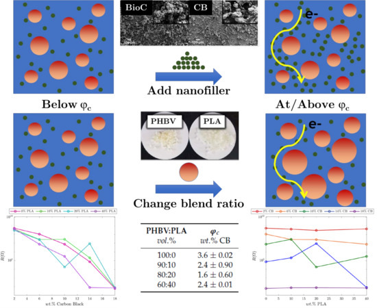
Biobased fillers, such as bio-derived cellulose, lignin byproducts, and biochar, can be used to modify the thermal, mechanical, and electrical properties of polymer composites. Biochar (BioC), in particular, is of interest for enhancing thermal and electrical conductivities in composites, and can potentially serve as a bio-derived graphitic carbon alternative for certain composite applications. In this work, we investigate a blended biopolymer system: poly(lactic acid) (PLA)/poly(hydroxybutyrate-co-hydroxyvalerate) (PHBV), and addition of carbon black (CB), a commonly used functional filler as a comparison for Kraft lignin-derived BioC. We present calculations and experimental results for phase-separation and nanofiller phase affinity in this system, indicating that the CB localizes in the PHBV phase of the immiscible PHBV:PLA blends. The addition of BioC led to a deleterious reaction with the biopolymers, as indicated by blend morphology, differential scanning calorimetry showing significant melting peak reduction for the PLA phase, and a reduction in melt viscosity. For the CB nanofilled composites, electrical conductivity and dynamic mechanical analysis supported the ability to use phase separation in these blends to tune the percolation of mechanical and electrical properties, with a minimum percolation threshold found for the 80:20 blends of 1.6 wt.% CB. At 2% BioC (approximately the percolation threshold for CB), the 80:20 BioC nanocomposites had a resistance of 3.43 × 10${}^8$ $\mathsf{\Omega }$ as compared to 2.99 × 10${}^8$ $\mathsf{\Omega }$ for the CB, indicating that BioC could potentially perform comparably to CB as a conductive nanofiller if the processing challenges can be overcome for higher BioC loadings.

1. Introduction

Increasing concern for the environment and volatile petroleum prices has led to growth of bio-based and biodegradable materials as alternatives to petroleum derived plastics [1]. Plastics from bio-derived sources, or bioplastics, can be processed from a variety of feedstock including raw and refined plant sources and methane gas from biological degradation processes [2]. One class of bioplastics, poly(hydroxyalkanoates) (PHAs), such as poly(hydroxybutyrate) (PHB) and its industrially-produced copolymer poly(hydroxybutyrate-co-hydroxyvalerate) (PHBV), is synthesized by microorganisms as a storage polymer and can be harvested to produce a usable plastic [3]. PHBV has mechanical properties most similar to polypropylene, however thermal processing of PHBV is challenging due the proximity of the thermal decomposition temperature to the melting temperature [4,5]. Poly(lactic acid) (PLA) is another important bioplastic, that can be produced through renewable resources, and has mechanical properties most similar to that of polystyrene [5]. Alone, both bioplastics are brittle, with relatively poor impact strength and low thermal degradation temperatures. The toughness and processability of these bioplastics can be improved through multiphase blends of PHBV and PLA, resulting in attractive material properties not obtainable in the neat biopolymers [2,6].

One growing application space for bioplastics is additive manufacturing, and an emergent area of this space is conductive filament. Conductive filament is used in the rapid prototyping and production of electrically conductive components on a variety of 3D printers [7,8]. This production method enables various applications from low cost sensors to conductive traces, branching into electromagnetic and radio frequency shielding [9,10]. Typically, conductivity in thermoplastics is achieved through the addition of a conductive filler, such as silver nanoparticles, carbon black nanofillers, or graphene [10,11]. In addition to electrical conductivity, these value-added composites can reduce cost and weight, add color, provide anti-static potential at low volume percent, and enhance the mechanical and thermal properties over that of the neat polymer [12]. Of these fillers, the majority of conductive filaments are produced with carbon black (CB), a commercially available petroleum-derived filler.

Though CB offers many positive benefits to polymer blends, when designing biobased composites having a renewable source for and considering the fate of filler materials is also important. Biochar (BioC) carries many of the same benefits as CB, but comes from renewable plant-derived sources and, as a widely applied agricultural amendment, is compatible with the bioplastic’s ability to biodegrade. This bio-sourced form of carbon is produced in a similar way to charcoal. Thermal decomposition of biomass in the absence of oxygen results in roughly 35% syngas, 30% bio-oil, and 35% BioC [13]. The electrical conductivity of lignin sourced BioC has been shown to improve with pyrolysis at high treatment temperatures (over 800 $°$C) [14,15,16].

The bulk of the work exploring conductive nanocomposites, including with polymer blends, consists of polymers mixed with CB, graphene, carbon nanotubes (CNTs), or other graphite fillers [7,8,17,18,19]. The conductivity of PLA-based composites has been successfully modified with CNTs [20,21], graphene [22,23,24,25], and CB [26,27]. Conductive filament made from PLA and conductive fillers (CB, graphene) is commercially available [28,29]. Fewer conductivity studies have been done with PHB and PHBV-based carbon nanocomposites; this work has been primarily with CNTs and graphene or graphene oxide, with conductivities in the range of ∼0.1 S/m to 30 S/m with loadings above the percolation threshold [30,31,32].

Studies of conductive polymer blends have shown that nanofillers lower the percolation threshold of the blend over that of nanofiller incorporated into a single polymer, due to the ability to reside in either the minor or major phase, or the interfacial region [19]. This partitioning of the nanofiller produces higher conductivity at lower weight percent filler than in their non-blended counterparts. Phase-separation has been used to control nanofiller localization in blended PLA composites [20,21,22,33]. Differences in nanofiller aspect ratio contribute to the phase-localization behavior in addition to phase separation in these composite blends [27,34,35]. The studies of BioC involve particulate in a single polymer, conductivity of non-incorporated monolithic BioC, or large (microns to millimeters) fillers in a polymer blend [12,14,36,37].

This study provides a novel investigation into the localization of CB and BioC nanofiller in biopolymer blends, and the resultant impact on mechanical and electrical properties of nanocomposites of interest for 3D printing. The focus is to investigate: (i) Nanofiller localization and resultant morphology in a blended biopolymer system, PHBV:PLA, (ii) electrical and mechanical percolation of the nanofilled composites, and (iii) the impact of the two nanofillers on processing and melt rheology. To elucidate how nanofiller localization would be expected to occur in the blends, we predict the interfacial energies of the blends using contact angle measurements and calculations of surface tension and verify these predictions using field emission scanning electron microscopy (FE-SEM). We then use impedance spectroscopy, Raman spectroscopy, and dynamic mechanical analysis (DMA) to evaluate the electrical and mechanical properties of the nanocomposites and calculate the percolation threshold in blended and non-blended systems. We use melt rheology during compounding and differential scanning calorimetry (DSC) to evaluate the impact of nanofiller addition during processing and how these interactions impact blend microstructure, thermal stability, and processability.

2. Theory

Polymer blend phase separation and incorporation of nanofillers can be described through the use of the Owens-Wendt theory [38]. The thermodynamics of phase behavior of polymers in a blend is governed by the surface tension of the polymers. The surface tension is comprised of polar and dispersive components, and is typically measured using the contact angle between the polymer surface and liquids with known polar and dispersive values. The Owens-Wendt theory combines the Goods Equation (1) with the Young’s Equation (2) to create the linear form (3) [38]:

$${\gamma }_{sl}={\gamma }_s+{\gamma }_l-2\sqrt{{\gamma }_l^d{\gamma }_s^d}-2\sqrt{{\gamma }_l^p{\gamma }_s^p}$$

(1)

$${\gamma }_s={\gamma }_{sl}+{\gamma }_{l}cos\left(\theta \right)$$

(2)

$${\displaystyle \frac{{\gamma }_{l}cos(\theta +1)}{2\sqrt{{\gamma }_l^d}}}={\gamma }_s^p{\displaystyle \frac{\sqrt{{\gamma }_l^p}}{\sqrt{{\gamma }_l^d}}}+\sqrt{{\gamma }_s^d}$$

(3)

Substituting into the linear form ($y=mx+b$) gives:

$$y={\displaystyle \frac{{\gamma }_{l}cos(\theta +1)}{2\sqrt{{\gamma }_l^d}}}$$

(4)

$$m={\gamma }_s^p$$

(5)

$$x={\displaystyle \frac{\sqrt{{\gamma }_l^p}}{\sqrt{{\gamma }_l^d}}}$$

(6)

$$b=\sqrt{{\gamma }_s^d}$$

(7)

where ${\gamma }_l$ is the overall surface tension of the wetting liquid, ${\gamma }_s$ is the overall surface energy of the solid, the polar and dispersive components are represented by ${\gamma }_s^p$,${\gamma }_l^p$ and ${\gamma }_s^d$, ${\gamma }_l^d$ respectively, ${\gamma }_{sl}$ represents the interfacial tension between the solid and the liquid, and $\theta$ is the contact angle between the liquid and the solid. A solid’s unknown polar and dispersive components (${\gamma }_s^p$,${\gamma }_s^d$) are calculated using contact angles with liquids of a known polar and dispersive component (${\gamma }_l^p$,${\gamma }_l^d$). This calculation is done by plotting contact angle data ($x,y$: Equations (4) and (6)) and using a line of best fit to determine a slope and y-intercept [39]. This form of the Harmonic Mean Method requires a minimum of two liquids for which surface tension data is well known to develop a best fit line.

In general, binary polymer blends exhibit either a blended morphology representative of miscibility, or they may exhibit a sea-island structure representative of an immiscible blend. For binary polymer composites, there are typically three potential locations of the nanofiller: It may exist in the major phase, the minor phase, or in the interfacial region between the two. The interfacial tension between the blended polymers and the nanoparticulates was calculated using the Harmonic Mean Equation (8), and used to predict the morphology of the system [39].

$${\gamma }_{ij}={\gamma }_i+{\gamma }_j-{\displaystyle \frac{4{\gamma }_i^d{\gamma }_j^d}{{\gamma }_i^d+{\gamma }_j^d}}-{\displaystyle \frac{4{\gamma }_i^p{\gamma }_j^p}{{\gamma }_i^p+{\gamma }_j^p}}$$

(8)

To determine miscibility of the polymer blend, the spreading coefficient ${\lambda }_{ij}$ was calculated for phase i on phase j (9). A positive ${\lambda }_{ij}$ indicates that polymer i will spread and is miscible on j, while a negative number indicates immiscibility between i on j [39].

$${\lambda }_{ij}={\gamma }_j-{\gamma }_i-{\gamma }_{ij}$$

(9)

The localization of the nanofiller in the blend can be predicted by determining the wetting coefficient of the polymer on the particulate, ${\omega }_{ij}$. This coefficient is given in Equation (10), where ${\gamma }_{i,NF}$ represents the interfacial tension of the nanofiller on polymer i [39].

$${\omega }_{ij}=\frac{{\gamma }_{i,NF}-{\gamma }_{j,NF}}{{\gamma }_{ij}}$$

(10)

By this definition, if ${\omega }_{ij}$ is greater than 1 the particulate will localize in the j phase of the polymer blend. In turn, if ${\omega }_{ij}$ is less than −1 it will localize in the i phase and finally if ${\omega }_{ij}$ is between 1 and −1 the particulate will localize in the interfacial region between the blends.

The contact angle between the polymers during molten flow can be characterized by Equation (11) and used to predict the shape of the minor phase in the major [39].

$${\theta }_{ij}=co{s}^{-1}\left(\frac{{\gamma }_j-{\gamma }_{ij}}{{\gamma }_i}\right)$$

(11)

3. Materials and Methods

3.1. Materials

Commercially available PHBV (ENMAT Y 1000p, >98% purity) in pellet form was provided by Tianan (Nigbo City, China). PLA (2003D), also in pellet form, was supplied by Nature Works (Minnetonka, MN, USA). Powdered CB (Vulcan XCMAX22) with a density of 0.19 g/cm${}^3$ was provided by Cabot Chemical Corporation (Boston, MA, USA). Kraft lignin, with a density of 1.3 g/cm${}^3$ at 25 $°$C, was purchased from Sigma-Aldrich, St. Louis, MO, USA and used to produce the BioC. All materials were stored in a desiccator prior to composite fabrication.

3.2. BioC Production

BioC was produced through slow pyrolysis of ball milled kraft lignin. Powdered kraft lignin (20 g) was milled with zirconia media for 24 h at 60 rpm. The media were removed and the milled lignin was stored at 105 $°$C to remove moisture. Prior to pyrolysis in a tube furnace, nitrogen gas was purged through the tube at 0.95 CCM for 15 min to establish an oxygen free environment. After the initial purging, nitrogen flow was reduced to 0.55 CCM and heating began at 10 $°$C/min to 750 $°$C. After one hour at 750 $°$C the temperature was ramped to 950 $°$C at a rate of at 10 $°$C/min and held for an hour. The sample was then allowed to cool to room temperature while still under nitrogen flow. Post pyrolysis, samples were stored at 105 $°$C.

3.3. Composite Fabrication

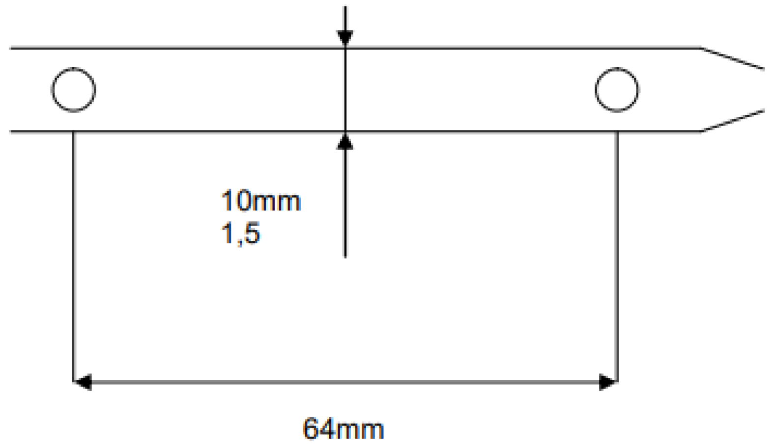
Composites were prepared by melt compounding in a Thermo Fisher Scientific HAAKE Minilab II dual screw extruder at 50 rpm and 190 $°$C for 5 min. During this time, rheology data were collected and viscosity was calculated from Minilab outputs as shown in Appendix B. After mixing, blends were extruded into a Thermo Fisher Scientific Minijet Pro injection molder. Initial injection pressure was 600 bar for 10 s followed by 450 bar for 60 s. Injection temperatures were 190 $°$C in the gun and 60 $°$C in the mold, as established through prior optimization. All composites were injected into a DMA sample mold (Thermo Fisher Scientific, Waltham, MA USA, Part # 557-2295) with dimensions of 60 × 10 × 1 mm${}^3$.

Table 1. PHBV:PLA composite blend ratios with CB and BioC nanofiller.

	Vol.% of Blend					wt.% of Total
PHBV	100	90	80	60	Nanofiller (CB, BioC)	2	6	10	14	18
PLA	0	10	20	40	PHBV:PLA blend	98	94	90	86	82

gives the blend ratios used for the PHBV:PLA blends and blends with nanofillers. CB nanofilled blends were made with all PHBV:PLA blend ratios, while samples of BioC were produced as feasible due to viscosity challenges during processing. Nanofiller was measured as a weight fraction of the total polymer blend.

3.4. Characterization

Interfacial parameters, polymer blend morphology, moduli, thermo-mechanical, and electrical properties were evaluated by video contact analysis, FE-SEM, DMA, DSC, Raman spectroscopy, and 4-point probe impedance spectroscopy measurements.

3.4.1. Contact Angle Analysis

To better understand the interactions of the polymer blends during mixing, polar and dispersive components of polymer surface tensions were calculated by measuring contact angles with deionized water and diiodomethane (MI). Contact angles were measured using a video contact angle system with drop sizes of 2.45 ± 0.5 $\mathsf{\mu }$L and a minimum of 5 measurements. Angles were divided into their dispersive and polar components using the Owens-Wendt relationship as described in Section 2 (Equations (1)–(3)).

Table 2. Surface tensions for water and diiomethane.

Liquid	$\mathbf{\gamma }$	${\mathbf{\gamma }}^{\mathit{p}}$	${\mathbf{\gamma }}^{\mathit{d}}$
Water	72.8	51.0	21.8
MI	50.8	0.4	50.4

shows the known dispersive and polar components of water and MI used as the contact liquid. Matlab code was developed to analyze the surface tensions and predict interfacial interactions, phase separation, and nanofiller localization in the polymer blends and nanofilled composites [40].

It is particularly difficult to consistently measure contact angles for nanofillers in order to determine surface energies. Instead, alternate methods such as absorption and heat of immersion are standard techniques and have been explored in previous studies which provided the literature values for CB used in this study [41,42].

3.4.2. Dynamic Mechanical Analysis

Dynamic mechanical measurements were conducted on a TA instruments Q800 DMA. A multi frequency-strain experiment in the 3-pt bending configuration was run at a frequency of 1 Hz, amplitude of 20 $\mathsf{\mu }$m, and a force track of 125%. The temperature was equilibrated at −40 $°$C for five minutes and increased to 150 $°$C at a constant rate of 5 $°$C/min. During the temperature ramp, storage modulus, loss modulus, and tan$\delta$ data were collected.

3.4.3. Differential Scanning Calorimetry

A TA Instruments Discovery DSC (Serial Number DSCI-0220) was used to assess the impact of the nanofillers on the polymers and blends. The nitrogen flow rate was 50 mL/min, as optimized in previous work [43]. Samples were encapsulated in aluminum pans with a target sample weight of 5 mg ± 2 mg, and heated from −20 $°$C to 180 $°$C in the first heating cycle at a rate of 10 $°$C/min. After equilibrating to 190 $°$C, they were held at 190 $°$C for 2 min prior to cooling at 10 $°$C/min to −20 $°$C. The samples were then heated at 10 $°$C/min to 195 $°$C in the second and final heating cycle. The glass transition temperature ($T_g$) was taken to be the midpoint of the heat capacity change, the melting temperature ($T_m$) was measured as the minimum of the endothermic peak upon heating, the cold crystallization temperature ($T_{cc}$) was measured as the maximum of the exothermic peak (when present) upon heating, and the crystallization temperature ($T_c$) was taken as the maximum temperature of the exothermic peak upon cooling (in between the first and second heating cycles).

The percent crystallinity of the PHBV and PLA in the matrix, ${\chi }_P$, was determined using a modification to the standard equation for single phase composites [44]:

$${\chi }_P[\%]=\frac{\Delta H_m-\Delta H_{cc}}{\Delta H_m^{\circ }}\left(\frac{1}{W_P}\right)·100\%$$

(12)

where $\Delta H_m$ and $\Delta H_{cc}$ are the enthalpies of melting and cold crystallization measured upon heating, $W_P$ is the weight fraction for the PHBV or PLA, and $\Delta H_m^{\circ }$) is the reference value for 100% crystalline polymer: 146 J/g or 12.5 kJ/mole [45,46] for PHB and 93.7 J/g for PLA [47]. As a reference, a typical value for the crystallinity of annealed PHB samples measured by Barham was 86% et al. [45]. To convert between volume and weight percent, densities of 1.24 g/cm${}^3$ for PHBV and 1.25 g/cm${}^3$ for PLA were used. Sample density was measured using a Mettler Toledo XS205DU Excellence series analytical balance with the Mettler Toledo Density determination kit for Excellence XP/XS analytical balances. The measurement is a buoyancy technique based on the Archimedes’ principle.

To evaluate the effect of BioC on each of the individual biopolymers, DSC was used to evaluate neat PHBV and PLA compared with each of the polymers with BioC. BioC was added on top of each of the biopolymers prior to the first heating cycle. The melting endotherms of the neat polymers were compared to the endotherms of the first and second heating cycles in the BioC nanofilled biopolymers.

3.4.4. Scanning Electron Microscopy

To obtain a cross section of the nanofilled blends, samples were cryo-fractured using liquid nitrogen. Examination of fracture surfaces though FE-SEM was conducted on a Supra 55VP System 2512 at 1 kV with an SE2 detector. Samples were uncoated. Nanofiller and matrix microstructure were characterized and the particle-matrix interfaces were imaged along with assessing potential localization of the nanofillers.

3.4.5. Impedance Spectroscopy

The polymers’ resistivity, impedance, capacitance, and phase angle were measured using a Hioki 3522-50 LCR HiTester in the 4 point configuration at room temperature. Each data point is the average of 3 measurements taken from 0.1 Hz to 10${}^5$ Hz. The percolation threshold for the composites was calculated using a Sigmoidal–Boltzmann function [48]:

$$\rho ={\rho }_l-\left(\frac{{\rho }_l-{\rho }_u}{1+e^{\frac{\phi -{\phi }_c}{\Delta \phi }}}\right)$$

(13)

where $\rho$ is the measured resistivity, ${\rho }_l$ is the lower limit for resistivity, ${\rho }_u$ is the upper limit for resistivity, $\phi$ is the percentage of CB in the blend, ${\phi }_c$ is the percolation threshold, and $\Delta \phi$ is the slope in proximity to the percolation threshold. The data for resistivity from impedance spectroscopy at 10${}^3$ Hz were fitted using the curve fitting toolbox in Matlab R2018b.

3.4.6. Raman Spectroscopy

A fully integrated high resolution Raman microscope for confocal Raman analysis, Horiba LabRam HR Evolution NIR, was used to evaluate CB, BioC, and nanofilled composites for graphitic content. The confocal microscope was used for optical images of the composite samples at 20× LWD and 50× LWD. During Raman spectral acquisition, Raman spectra were acquired at 50× LWD and 100×, the stigmatic spectrometer was used with a grating of 1800 gr/mm, and the 532 nm 100 mW laser at 1%. To reduce the impact of heating in the samples, the acquisition time was 3 s, and the spectra were accumulated for 3 acquisitions. Raman spectra were recorded between 1000 and 1800 cm${}^{-1}$, which corresponds to the spectral region that provides data on the microstructure of carbons giving a measure of the graphite band at 1530–1610 cm${}^{-1}$ (G) and the disorder-induced band at 1320–1370 cm${}^{-1}$ (D) [23,49,50]. The cftool in Matlab was used to fit gaussian exponentials to the CB and BioC peaks observed in this region to determine the peak locations for D and G peaks and the intensity ratio, $\raisebox{1ex}{$I_D$}\!\left/ \!\raisebox{-1ex}{$I_G$}\right.$ [51].

4. Results and Discussion

4.1. Evaluation of Blend Morphology and Nanofiller Localization

4.1.1. Predictions from Interfacial Tension

Contact angle analysis with water revealed that the two polymers exhibit hydrophilic characteristics as contact angles were below 90$°$. In addition, evaluation with MI showed that both PHBV and PLA exhibit dispersive dominate components (

Table 3. Contact angles and surface tensions using the Owens-Wendt model.

	Contact Angles		Surface Tensions
	$\mathbf{\theta }$H${}_{\mathbf{2}}$O	$\mathit{\theta }$MI	$\mathbf{\gamma }$(20$°$C)	$\mathbf{\gamma }$ (190 $°$C)	${\mathbf{\gamma }}^{\mathit{d}}$	${\mathbf{\gamma }}^{\mathit{p}}$
	deg$°$	deg$°$	(mJ/m${}^{\mathbf{2}}$)	(mJ/m${}^{\mathbf{2}}$)	(mJ/m${}^{\mathbf{2}}$)	(mJ/m${}^{\mathbf{2}}$)
PHBV	64.55 ± (1.06)	47.24 ± (0.98)	45.095	35.195	32.365	12.729
PLA	64.00 ± (0.66)	62.02 ± (3.05)	40.996	31.096	23.892	17.104
CB [41,42]	-	-	98.1	87.9	84.1	3.2

).

Table 4. Interfacial tension and spreading coefficients between polymers and nanofiller.

Component	Interfacial Tension	Blend (i:j)	Spreading	${\mathbf{\theta }}_{\mathit{ij}}^{\mathit{o}}$	Wetting	Particulate
	$\frac{\mathit{mN}}{\mathit{m}}$		Coef		Coef	Localization
PHBV/PLA	1.924	PHBV:PLA	−6.0072	29.918	−7.4971	PHBV
PHBV/CB	5.187	PLA:PHBV	2.1592	150.08	7.4971	PHBV
PLA/CB	8.682

shows predictions of miscibility of the polymer blends and the localization of the nanofiller within the blends made from Equations (9) and (10). A negative spreading coefficient between PHBV on PLA suggests that the PHBV phase is immiscible with the PLA phase. The tension between the CB and PHBV is significantly lower than that between the CB and PLA, suggesting that the CB will preferentially localize in the PHBV phase. This predicted separation is further supported by the negative wetting coefficient between CB on the PHBV major phase, and a positive wetting coefficient with the PLA major phase. These equations predict that for the blends studied here, PLA will form an immiscible structure within PHBV while CB will reside in the PHBV phase.

4.1.2. Verification of Nanofiller Partitioning and Blend Morphology

Figure 1 shows FE-SEM micrographs of an 80:20 PHBV:PLA blend with and without CB and BioC nanofiller. Immiscibility of PLA in PHBV is seen in its sea-island structure (Figure 1a), as predicted by the surface tension results. As CB is added to the blend (Figure 1b), it appears to localize in the major PHBV phase while the PLA phase is left absent of nanofiller. This morphology observed via FE-SEM shows a granularity characteristic of the CB nanofiller, and is comparable to other studies where SEM observation of carbon black localization was verified with transmission electron microscopy (TEM) [52,53]. Furthermore, the addition of CB does not alter the immiscibility of the two polymers. The effects of adding BioC to the blend can be seen in Figure 1c. In the blend with BioC, there is no visual distinction between the two polymer phases. Based on this observation and additional supporting evidence through mixing experiments, rheology, and DSC, we hypothesize that BioC reacts with the biopolymers, potentially preferentially depolymerizing the PLA phase. Previous studies have observed that reduced molecular weight PLA is miscible in PHBV and vice versa [54,55,56,57,58]. Therefore, the lack of observable phase separation in FE-SEM is potentially indicative of this molecular weight reduction. In summary, the partitioning of the CB nanofiller behaves as predicted. The interactions of the BioC with the polymer blend are more complex and are discussed in additional detail in Section 4.3.1 and Section 4.3.2.

For the surface energy and partitioning predictions made in Section 4.1 to be accurate, the filler particle size should be smaller than the minor phase regions of the blend. The as-received lignin yielded BioC with an average particle size of approximately 100 $\mathsf{\mu }$m, larger than the 1–3 $\mathsf{\mu }$m domains of the PLA in the PHBV (Figure 1a,b and Figure 2a). The milled lignin yields BioC with a comparable particle size to that of the CB (Figure 2). This nano size enables the filler material to reside in either the minor or the major phase of the blend.

4.2. Electrical and Mechanical Percolation of Nanofillers

4.2.1. Impedance Spectroscopy of Polymer Blends

Impedance ($\mathit{Z}$) is defined as the effective resistance of a component to an alternating current made up of real (Z’) and imaginary ($Z”$) components ($Z=Z’+jZ”$). The real and imaginary components of impedance are classified as resistance and reactance respectively. As frequency is increased, Z’ will rapidly decrease in insulators and remain constant in conductive materials. Figure 3 shows the resistance ($R$), and impedance, $Z$, by weight percent CB (Figure 3a,b) and by volume percent PLA (Figure 3c,d). Figure A3 in Appendix C.1 shows the full spectrum data collected from impedance spectroscopy.

For blends with CB filler content below 18%, there is a significant decrease in $Z$ around frequencies of ${10}^4$ Hz (shown in Figure A3). This frequency is considered the characteristic frequency ($f_c$) at which a dependency on frequency forms. Insulators below $f_c$ behave independently of frequency until frequency is increased above $f_c$ where they become frequency dependent. Samples above 18% CB did not experience this drop off and were considered to behave independent of frequency.

As expected, increasing the percentage of CB added to the matrix increased the conductivity of the nanofilled blend. Using the Sigmoidal-Boltzmann function to fit the resistivity showed that with increasing volume percent of PLA, the percolation threshold (${\phi }_c$) shifted from 3.6% in neat PHBV to a minimum of 1.6% for 80:20 PHBV:PLA.

Table 5. Percolation threshold, ${\phi }_c$, with volume percent PLA.

PHBV:PLA	${\mathbf{\phi }}_{\mathit{c}}$
vol.%	wt.% CB
100:0	3.6 ± 0.02
90:10	2.4 ± 0.90
80:20	1.6 ± 0.60
60:40	2.4 ± 0.01

gives the values for ${\phi }_c$ with the PLA percentage of the blend. Depending on the conditions for the selective localization of CB at the interface or in one of the polymer phases, in this case PHBV, ${\phi }_c$ changes with the relative amounts of the polymer phases in the system [59,60]. Other researchers have seen a similar optimization in the mechanical properties for a related 80:20 system [61].

The 80:20 PHBV:PLA 2% BioC sample that was fabricated and measured, had a resistance of 3.43 × 10${}^8$ $\mathsf{\Omega }$ as compared to 2.99 × 10${}^8$ $\mathsf{\Omega }$ for the 2% CB samples, indicating that BioC has the potential to perform similarly to CB when the BioC is produced via the method described herein, provided that challenges during composite fabrication (Section 4.3.1) can be overcome. Converting the measured resistance to resistivity, at 18 wt.% CB the resistivity of the PHBV:PLA nanocomposites ranges from 128 $\mathsf{\Omega }·$cm to 167 $\mathsf{\Omega }·$cm, which is comparable to commercially available filament (∼0.5–115 $\mathsf{\Omega }·$cm) [28,29].

4.2.2. Polymer-Nanofiller Interactions

Raman spectroscopy provided insight both into the graphitic content of the BioC as well as the polymer-nanofiller interface in the blends.

Table 6. Graphitic (G) and disordered (D) bands and peak intensity ratio ($\raisebox{1ex}{$I_D$}\!\left/ \!\raisebox{-1ex}{$I_G$}\right.$) in CB and BioC nanofilled blends.

	D	G	$\raisebox{1ex}{${\mathit{I}}_{\mathit{D}}$}\!\left/ \!\raisebox{-1ex}{${\mathit{I}}_{\mathit{G}}$}\right.$
	(1320–1370 cm${}^{-1}$)	(1530–1610 cm${}^{-1}$)
CB [49]	1359	1604	1.12
BioC	1366	1534	1.13
80:20, 6% CB	1342	1599	1.08
80:20, 6% BioC	1368	1573	1.03

gives the D and G bands for BioC as compared to previously characterized CB [49]. As expected, for both CB and BioC, only partial graphitization is present, as evidenced by the contribution of the D band which corresponds $s{p}^3$ carbon and is attributed to a higher proportion of defects [50,62]. The intensity ratio between the D and G bands ($\raisebox{1ex}{$I_D$}\!\left/ \!\raisebox{-1ex}{$I_G$}\right.$) is similar between CB and BioC, potentially indicating similarities in the graphitic and disordered carbon content, although this relationship is complex and is also linked to pyrolysis conditions [63,64,65]. Raman spectroscopy does support the formation of $s{p}^2$ states in the lignin-derived BioC which contribute to electrical conductivity.

Raman spectra provide insight into the polymer-nanofiller interaction via excitation energy shifts upon being incorporated into composites [66]. The Raman spectra corresponding to the D and G bands of both nanofillers were clearly observable in the composites. The CB nanofilled composites had a minimal downshift in the G and D peak intensities upon incorporation of the CB. The BioC showed a more significant upshift in the G band of 39 cm${}^{-1}$. This G-band shift is often observed in chemical modification of the carbon, the presence of electron-donor or acceptor impurities, and surface interactions at the polymer-filler interface [66,67]. Given that there is a complex relationship between the biopolymers and the lignin-derived BioC (Section 4.3), this shift can likely be attributed to that interaction.

4.2.3. Dynamic Mechanical Analysis

Figure 4 shows the mechanical analysis of a subset of the PHBV:PLA:CB nanocomposites for blends below or near the percolation threshold (2% CB) and above the percolation threshold (10% CB). At low temperatures, below the $T_g$ for PLA, there is an increase in elastic modulus of ∼5500 MPa ± 1695 MPa for the high versus low nanofilled composites. This increase is likely due to the combined increase in PHBV and PLA crystallinity between the 2% and 10% CB composites (Section 4.3.2). At high temperatures, the storage modulus of the composites is primarily affected by the blend ratio (PHBV:PLA).

The loss modulus is related to the material’s ability to dissipate mechanical energy and the loss tangent (tan$\delta$), or the ratio between the loss and storage moduli, is related to damping. In composites, these values can be linked to interfacial interactions and toughness [68,69]. Both were influenced by the CB content and blend ratio, with the loss modulus at high temperature increasing slightly in the high nanofilled composites while decreasing with increasing PLA content. There is not a clear dependence of tan$\delta$ on CB or blend ratio except for around $T_g$. All blends show a prominent peak in tan$\delta$ around 65.5 ${}^{\circ }$C ± 2.3 $°$C for 2% CB and shifted upwards to 70.4 ${}^{\circ }$C ± 1.3 $°$C for 10% CB. The observed peak is near the $T_g$ for PLA, however as even the 100% PHBV composite shows this peak, there is also a contribution due to the presence of the nanofiller. For blends with PLA, the magnitude of the tan$\delta$ peak decreased between the low and high CB composites, indicating that the presence of additional nanofiller reduced material damping around $T_g$. For all of the blends there was a shift in tan$\delta$ towards higher temperatures with increasing CB content, which can be attributed to the increased nanofiller content inhibiting chain movement [70,71]. This shift can also indicate increased thermal stability in the nanofilled composites. The nanofilled composites also improved temperature stability in the loss and storage moduli over that of neat PHBV (data not shown), which started to decrease around 105 $°$C as compared to ∼120 $°$C for the nanofilled composites. Like the electrical percolation of the nanofiller through the polymer blends, the increases in storage modulus and tan$\delta$ can be linked to the intercalation of the nanofiller through the matrix.

4.3. Nanofillers and Fabrication

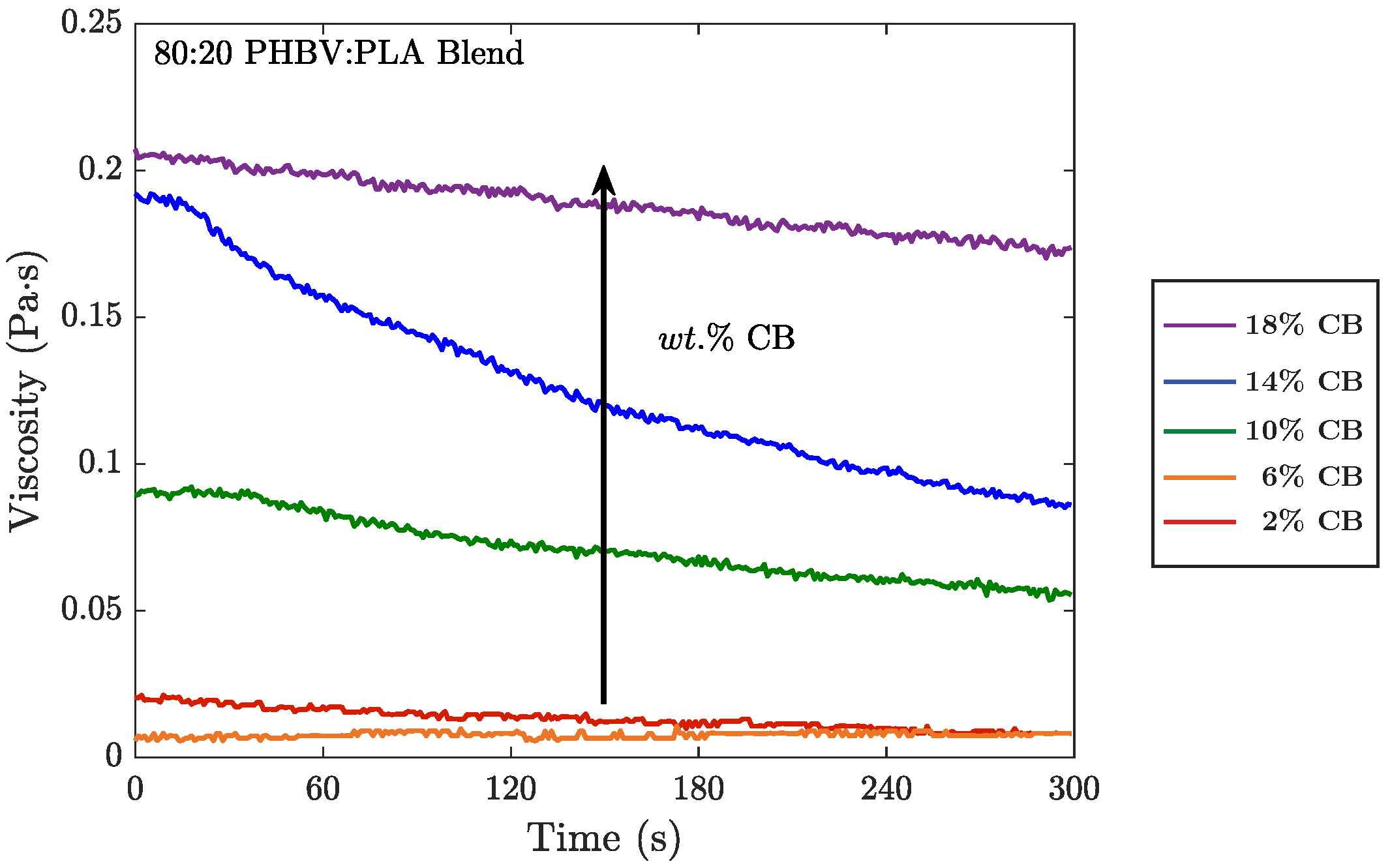
The behavior of the nanofillers during fabrication was highly dependent on the nanofiller type, CB or BioC. Melt rheology during compounding showed that the melt viscosity of the CB blends increased with increasing nanofiller content, while the viscosity of the BioC blends decreased significantly with the addition of the nanofiller. This effect became more pronounced with increased addition of BioC. DSC showed a modest effect on the melting temperature ($T_m$) and crystallinity ($\chi$) upon the addition of CB to the blends. In the case of BioC, the addition of small amounts of nanofiller had a pronounced effect on both $T_m$ and $\chi$.

4.3.1. Rheology During Extrusion

In addition to modifying the electrical and mechanical properties of the solid composites, the nanofillers had disparate effects on the melt rheology of the blends during mixing. For CB, the rheology measurements during the mixing cycle of the extruder were largely as expected. Early in the mixing cycle, viscosity peaks prior to full mixing of the nanofilled biopolymer blends. As filler and polymers mix, the viscosity of the system begins to decrease until it plateaus. This plateau indicates that the nanofillers are incorporated and melt blending has stabilized, which occurred by 5 min for all CB samples. Also as expected, as CB increased in the blends, the melt became more viscous (Figure 5). This effect is attributed to the added amount of filler in the mixture. Alternatively, the viscosity of BioC blends drops to zero nearly immediately as the filler is added, resulting in a polymer blend that is too fluid for extrusion and injection molding. Due to this rapid reduction in melt viscosity and underlying material causes for the reduced viscosity, BioC nanofilled blends above 2 wt.% could not reproducibly be processed into dimensionally stable composites. The unexpected effect of the BioC on melt viscosity is likely due to chemical reactions with the polymer matrix, as described in Section 4.3.2 and Appendix A.

4.3.2. Differential Scanning Calorimetry

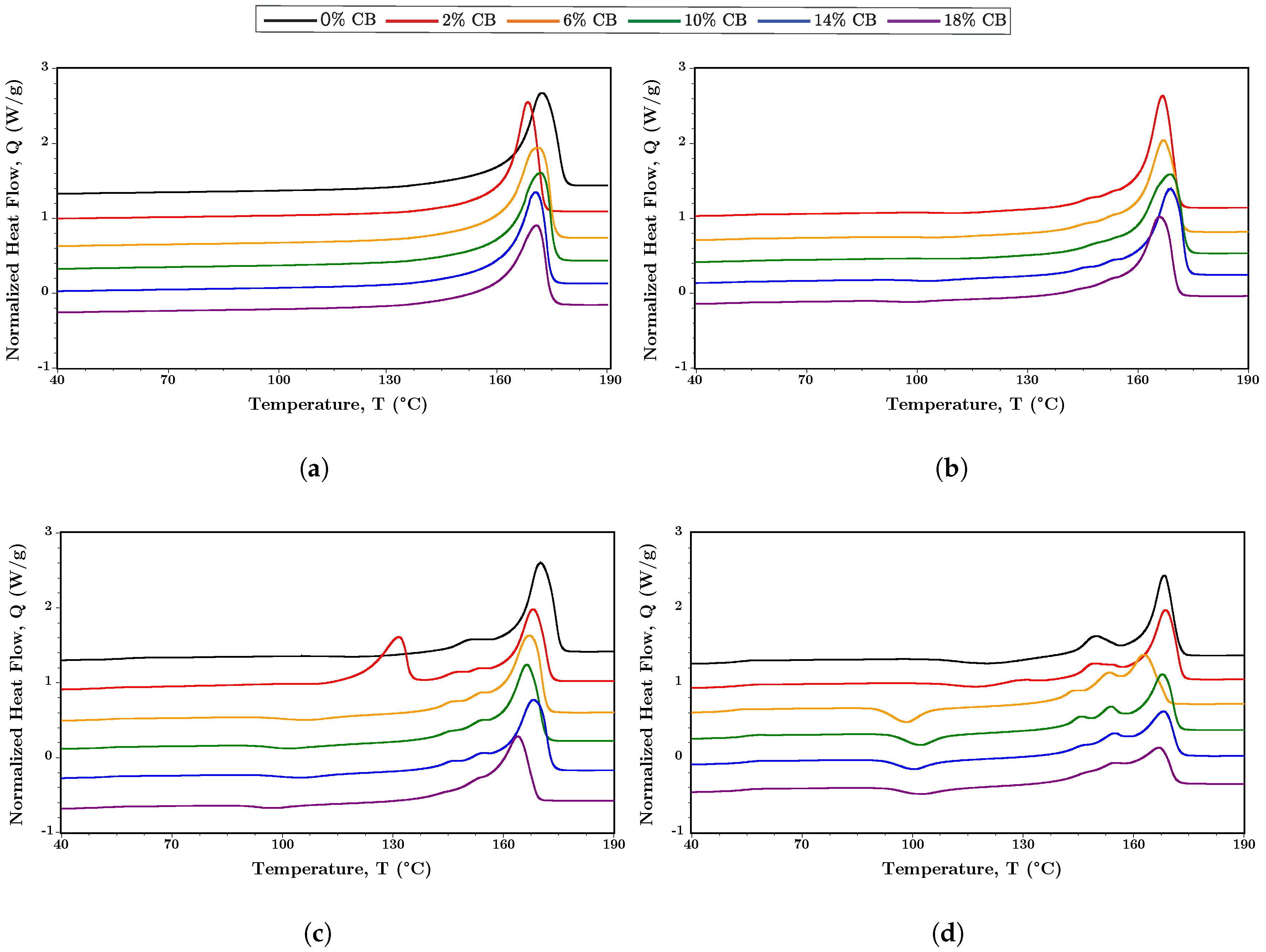
Figure 6 shows the DSC results for the melting peaks of the blended polymers with increasing wt.% CB. In Figure 6a for neat PHBV with CB, the melting peak shifts slightly towards lower temperatures with increasing CB. With increasing PLA content in the blend, Figure 6b–d, the impact on the melting behavior becomes more pronounced. Figure 6d for the blend (black line) clearly displays the split melting peak, PHBV (170.1 $°$C) and PLA (149.3 $°$C), anticipated for a phase-separated blend [6,57,69]. With increasing CB, there is a reduction in the main melting peak areas for both components, which results in a decrease in crystallinity, $\chi$, attributed to these primary peaks. This reduction is shown in Figure 7a (solid lines, PLA 10–40%), with the reduction of $\chi$ for PHBV. After an initial increase at low CB%, the crystallinity of the PLA phase remains largely unchanged with increasing CB, Figure 7a (dashed lines), due in part to attributing the shoulder peaks to the PLA phase. This increase in peak shoulders and the shift toward lower temperatures (e.g., Figure 6d) is indicative of decreased crystallite size and order likely due either to molecular weight reduction in the PHBV component, PLA component or both, or nanofiller-induced disruption of the crystalline phases [8,43,72].

Another feature, most clearly observable for Figure 6c,d, is the presence of a cold crystallization peak, which is most pronounced for CB wt.% of 10% and above. This peak shows a general trend of shifting towards lower temperature with increased CB (Figure 7b, dashed lines). The presence of cold crystallization indicates barriers to full crystallization during cooling. Because PLA has a cold crystallization peak in the region of the transition observed in the nanofilled composites, we attribute this cold crystallization to the PLA phase (Appendix C.2,

Table A1. Differential scanning calorimetry of the PHBV:PLA blended polymers.

Composition	Filler	${\mathit{T}}_{\mathit{g}}$	${\mathit{T}}_{\mathit{cc}}$	${\mathit{T}}_{\mathit{c}}$ PHBV:PLA	${\mathit{T}}_{\mathit{m}}$	$\mathbf{\Delta }{\mathit{H}}_{\mathit{m}}$	$\mathbf{\Delta }{\mathit{H}}_{\mathit{cc}}$	${\mathit{X}}_{\mathit{c}}$
	wt.% CB	$°$C	$°$C	$°$C	$°$C	$\mathit{J}/\mathit{g}$	$\mathit{J}/\mathit{g}$	%
100:0	0	-	-	122	172	92.0	-	63
100:0	2	-	-	126	169	81.7	-	57
100:0	6	-	-	125	171	89.7	-	65
100:0	10	-	-	125	172	85.1	-	65
100:0	14	-	-	126	171	81.8	-	65
100:0	18	-	-	124	171	76.6	-	64
PLA Component
90:10	2	51.97	113.44	-	152.00	16.24	3.47	13.6
90:10	8	51.36	107.90	-	152.00	16.11	3.38	13.6
90:10	10	54.12	113.29	-	152.00	14.00	3.46	11.2
90:10	14	51.69	104.55	-	152.00	12.70	1.76	11.7
90:10	18	51.28	99.41	-	152.00	16.73	1.79	15.9
80:20	0	57.21	123.17	-	150.00	10.52	3.31	7.7
80:20	2	52.30	0.00	-	153.00	10.46	0.00	7.9
80:20	8	53.19	106.57	-	153.00	14.87	3.04	12.0
80:20	10	53.44	102.46	-	153.00	14.83	3.60	13.2
80:20	14	53.30	105.28	-	153.00	12.56	2.47	11.7
80:20	18	52.18	97.80	-	153.00	16.65	1.60	7.5
60:40	0	52.37	121.60	-	149.00	14.59	9.59	5.3
60:40	2	52.65	117.85	-	153.00	14.06	5.79	8.8
60:40	8	50.66	98.54	-	153.00	21.85	9.39	13.3
60:40	10	53.76	102.00	-	153.00	16.01	7.05	9.6
60:40	14	54.58	100.48	-	155.00	15.30	6.26	9.7
60:40	18	53.74	102.22	-	155.00	14.88	4.08	11.5
PHBV Component
90:10	2	-	-	125.74	166.88	69.88	-	47.87
90:10	8	-	-	125.13	167.04	65.32	-	44.74
90:10	10	-	-	125.71	169.04	63.78	-	43.69
90:10	14	-	-	125.24	169.08	61.20	-	41.92
90:10	18	-	-	124.74	166.15	55.40	-	37.95
80:20	0	-	-	119.03	170.08	63.96	-	43.81
80:20	2	-	-	125.00	168.03	48.57	-	33.27
80:20	8	-	-	124.83	167.17	55.44	-	37.98
80:20	10	-	-	124.18	166.39	51.97	-	35.60
80:20	14	-	-	124.84	168.13	53.26	-	36.48
80:20	18	-	-	123.14	163.81	40.38	-	27.66
60:40	0	-	-	116.37	168.42	45.85	-	31.40
60:40	2	-	-	123.30	168.72	45.40	-	31.10
60:40	8	-	-	121.96	163.05	30.89	-	21.16
60:40	10	-	-	123.40	167.79	37.18	-	25.47
60:40	14	-	-	121.60	168.12	34.13	-	23.38
60:40	18	-	-	119.65	166.85	28.82	-	19.74

) [73]. The presence of cold crystallization with increased CB supports nanofiller disruption of the crystallization process in the blends. Appendix C.2, Table A1 gives the complete DSC data for the CB nanofilled blends.

In addition to the reduction in crystallinity in the PHBV phase due to the CB content, there is a more pronounced reduction with the increase in PLA content. Also, while the PLA phase shows a reduction in the cold crystallization peak, the crystallization peak of the blend has an initial increase due to the presence of the nanofiller and then remains largely independent of CB content. Therefore, while $\chi$ shows some effect due to the nanofiller, the PHBV phase is influenced primarily by the vol.% of PLA. Toughness and physical effects of aging in PHBV:PLA blends have been shown to improve above that of the neat polymers, because of this tailoring of crystallinity and phase interactions, indicating the potential of these blends for enhanced stability and mechanical properties [58,61].

In contrast, the effects of adding BioC to the blends were significantly different. As discussed in Section 4.3.1, when added to the melt, the viscosity decreased substantially. To explore this effect, Figure 8 shows a comparison between neat PHBV, neat PLA, and BioC added to PHBV and PLA prior to the heating cycles in the DSC. BioC has a substantial effect on the melting endotherm for both PLA and PHBV. PLA:BioC exhibits a melting peak around 150 $°$C on the first cycle, as would be expected in neat PLA. PHBV:BioC also has a melting peak similar to the neat polymer on the first cycle. After mixing with BioC and undergoing a thermal cycle, PLA:BioC exhibits no melt peak implying that PLA no longer has crystalline regions. A similar effect takes place in the PHBV:BioC, with a significant reduction in the area of the peak. These results indicate that the significant material changes in the blend upon addition of this lignin-based BioC are likely due to a reaction between the BioC and the polymers. This reaction renders use of BioC prepared from this source difficult for use in extrusion and injection molding. Additional evidence of this reaction is given in Appendix A, Figure A1.

5. Conclusions

Conductive nanofiller localization was tailored through phase separation in the PHBV:PLA blends. The partitioning of the nanofiller for the phase-separated morphology of the blends was calculated from surface energies derived from contact angle analysis. FE-SEM was used to verify the location of the nanofillers; CB localized within the PHBV phase as predicted by our calculations. The lignin-derived BioC had a more complex reaction with the biopolymers, as evidenced by the change in blend morphology as observed via FE-SEM, a rapid reduction in melt upon addition of BioC, and DSC results that show a significant reduction in the PHBV melting peak and the absence of a melting peak for the PLA phase. These material changes upon the addition of BioC are likely due to a reaction occurring between the biopolymers and BioC, potentially due to residual species from the Kraft lignin process. The rapid reduction in melt viscosity and source of lignin-BioC/polymer interaction will be critical to implementing BioC as a potential alternative to CB.

The impedance of CB in PHBV:PLA blends was measured for weight percentages of 0, 2, 6, 10, 14, and 18 wt.% CB and PHBV:PLA blends of 100:0, 90:10, 80:20, and 60:40. The phase-separated blends also modified the percolation threshold, which varied between 3.6% and 1.6% CB with the maximum value for 100% PHBV and the minimum for the 80:20 blend. When comparing CB composites with BioC composites with 2% nanofiller (approximately at the percolation threshold), the 2% BioC had a resistance of 3.43 × 10${}^8$ $\mathsf{\Omega }$ as compared to 2.99 × 10${}^8$ $\mathsf{\Omega }$ for the CB, indicating that BioC could perform comparably to CB as a conductive nanofiller if the processing challenges can be overcome. Results at higher BioC loading would be required to establish if this comparable behavior is present for more conductive samples. Both nanofillers exhibited graphitic content individually and incorporated into PHBV:PLA blends, as determined via Raman spectroscopy, which is necessary for a conductive network of nanoparticles. These results further support the use of nano sized lignin-derived BioC as an electrically conductive nanofiller in biocomposites.

References

- Pilla, S. Handbook of Bioplastics and Biocomposites Engineering Applications; Wiley: Hoboken, NJ, USA, 2011; p. 588. [Google Scholar]
- Smith, R. Biodegradable Polymers for Industrial Applications; Woodhead: Sawston/Cambridge, UK, 2005; p. 531. [Google Scholar]
- Pieja, A.J.; Rostkowski, K.H.; Criddle, C.S. Distribution and selection of poly-3-hydroxybutyrate production capacity in methanotrophic proteobacteria. Microb. Ecol. 2011, 62, 564–573. [Google Scholar] [CrossRef] [PubMed]
- Tsui, A.; Wright, Z.C.; Frank, C.W. Biodegradable polyesters from renewable resources. Annu. Rev. Chem. Biomol. Eng. 2013, 4, 143–170. [Google Scholar] [CrossRef] [PubMed]
- Mekonnen, T.; Mussone, P.; Khalil, H.; Bressler, D. Progress in bio-based plastics and plasticizing modifications. J. Mater. Chem. A 2013, 1, 13379–13398. [Google Scholar] [CrossRef]
- Nanda, M.R.; Misra, M.; Mohanty, A.K. The effects of process engineering on the performance of PLA and PHBV blends. Macromol. Mater. Eng. 2011, 296, 719–728. [Google Scholar] [CrossRef]
- Foster, C.W.; Down, M.P.; Zhang, Y.; Ji, X.; Rowley-Neale, S.J.; Smith, G.C.; Kelly, P.J.; Banks, C.E. 3D printed graphene based energy storage devices. Sci. Rep. 2017, 7, 42233. [Google Scholar] [CrossRef] [PubMed]
- Wei, X.; Li, D.; Jiang, W.; Gu, Z.; Wang, X.; Zhang, Z.; Sun, Z. 3D printable graphene composite. Sci. Rep. 2015, 5, 11181. [Google Scholar] [CrossRef]
- Marasso, S.L.; Cocuzza, M.; Bertana, V.; Perrucci, F.; Tommasi, A.; Ferrero, S.; Scaltrito, L.; Fabrizio Pirri, C.; Pirri, C.F. PLA conductive filament for 3D printed smart sensing applications. Rapid Prototyp. J. 2018, 24, 739–743. [Google Scholar] [CrossRef]
- Flowers, P.F.; Reyes, C.; Ye, S.; Kim, M.J.; Wiley, B.J. 3D printing electronic components and circuits with conductive thermoplastic filament. Addit. Manuf. 2017, 18, 156–163. [Google Scholar] [CrossRef]
- Wang, X.; Jiang, M.; Zhou, Z.; Gou, J.; Hui, D. 3D printing of polymer matrix composites: A review and prospective. Compos. Part B Eng. 2017, 110, 442–458. [Google Scholar] [CrossRef]
- Snowdon, M.R.; Mohanty, A.K.; Misra, M. Miscibility and performance evaluation of biocomposites made from polypropylene/poly(lactic acid)/poly(hydroxybutyrate-co-hydroxyvalerate) with a sustainable biocarbon filler. ACS Omega 2017, 2, 6446–6454. [Google Scholar] [CrossRef]
- Lehmann, J.; Joseph, S. Biochar for Environmental Management: Science and Technology; Earthscan: London, UK, 2009; p. 416. [Google Scholar]
- Gabhi, R.S.; Kirk, D.W.; Jia, C.Q. Preliminary investigation of electrical conductivity of monolithic biochar. Carbon 2017, 116, 435–442. [Google Scholar] [CrossRef]
- Palapati, N.; Demir, M.; Harris, C.T.; Subramanian, A.; Member, I.; Gupta, R. Enhancing the electronic conductivity of lignin-sourced, sub-micron carbon particles. In Proceedings of the 2015 IEEE Nanotechnology Materials and Devices Conference (NMDC), Anchorage Alaska, 13–16 September 2015; pp. 1–2. [Google Scholar]
- You, X.; Misra, M.; Gregori, S.; Mohanty, A.K. Preparation of an electric double layer capacitor (EDLC) using Miscanthus-derived biocarbon. ACS Sustain. Chem. Eng. 2018, 6, 318–324. [Google Scholar] [CrossRef]
- Yuan, Q.; Wu, D. Low percolation threshold and high conductivity in carbon black filled polyethylene and polypropylene composites. J. Appl. Polym. Sci. 2010, 115, 3527–3534. [Google Scholar] [CrossRef]
- Gao, H.; Meisel, N.A. Exploring the manufacturability and resistivity of conductive filament used in material extrusion additive manufacturing. In Proceedings of the 28th Annual International Solid Freeform Fabrication Symposium, Austin, TX, USA, 7–9 August 2017; pp. 1612–1626. [Google Scholar]
- Zhang, Q.; Zhang, B.Y.; Guo, Z.X.; Yu, J.; Zhang, Q.; Zhang, B.Y.; Guo, Z.X.; Yu, J. Tunable electrical conductivity of carbon-black-filled ternary polymer blends by constructing a hierarchical structure. Polymers 2017, 9, 404. [Google Scholar] [CrossRef]
- Wu, D.; Zhang, Y.; Zhang, M.; Yu, W. Selective localization of multiwalled carbon nanotubes in poly(ϵ-caprolactone)/polylactide blend. Biomacromolecules 2009, 10, 417–424. [Google Scholar] [CrossRef] [PubMed]
- Laredo, E.; Grimau, M.; Bello, A.; Wu, D.F.; Zhang, Y.S.; Lin, D.P. AC conductivity of selectively located carbon nanotubes in poly(ϵ-caprolactone)/polylactide blend nanocomposites. Biomacromolecules 2010, 11, 1339–1347. [Google Scholar] [CrossRef]
- Qi, X.Y.; Yan, D.; Jiang, Z.; Cao, Y.K.; Yu, Z.Z.; Yavari, F.; Koratkar, N. Enhanced electrical conductivity in polystyrene nanocomposites at ultra-low graphene content. ACS Appl. Mater. Interfaces 2011, 3, 3130–3133. [Google Scholar] [CrossRef]
- Shen, Y.; Jing, T.; Ren, W.; Zhang, J.; Jiang, Z.G.; Yu, Z.Z.; Dasari, A. Chemical and thermal reduction of graphene oxide and its electrically conductive polylactic acid nanocomposites. Compos. Sci. Technol. 2012, 72, 1430–1435. [Google Scholar] [CrossRef]
- Kim, I.H.; Jeong, Y.G. Polylactide/exfoliated graphite nanocomposites with enhanced thermal stability, mechanical modulus, and electrical conductivity. J. Polym. Sci. Part B Polym. Phys. 2010, 48, 850–858. [Google Scholar] [CrossRef]
- Sabzi, M.; Jiang, L.; Liu, F.; Ghasemi, I.; Atai, M. Graphene nanoplatelets as poly (lactic acid) modifier: Linear rheological behavior and electrical conductivity. J. Mater. Chem. A 2013, 1, 8253–8261. [Google Scholar] [CrossRef]
- Wu, D.; Lv, Q.; Feng, S.; Chen, J.; Chen, Y.; Qiu, Y.; Yao, X. Polylactide composite foams containing carbon nanotubes and carbon black: Synergistic effect of filler on electrical conductivity. Carbon 2015, 95, 380–387. [Google Scholar] [CrossRef]
- Xiu, H.; Zhou, Y.; Huang, C.; Bai, H.; Zhang, Q.; Fu, Q. Deep insight into the key role of carbon black self-networking in the formation of co-continuous-like morphology in polylactide/poly(ether)urethane blends. Polymer 2016, 82, 11–21. [Google Scholar] [CrossRef]
- BlackMagic3D Conductivity. Available online: https://www.blackmagic3d.com/Conductive-p/grphn-pla.htm (accessed on 19 November 2018).
- Proto-Pasta Conductivity. Available online: https://www.proto-pasta.com/pages/conductive-pla#CCcoductivity (accessed on 19 November 2018).
- Thinh, P.X.; Basavaraja, C.; Kim, K.I. Fabrication and characterization of honeycomb-patterned film from poly (ϵ-caprolactone)/poly ((R)-3-hydroxybutyric acid)/reduced graphene oxide composite. Polym. J. 2013, 45, 1064. [Google Scholar] [CrossRef]
- Dan, L.; Pope, M.A.; Elias, A.L. Solution-processed conductive biocomposites based on polyhydroxybutyrate and reduced graphene oxide. J. Phys. Chem. C 2018, 122, 17490–17500. [Google Scholar] [CrossRef]
- Arza, C.R.; Jannasch, P.; Maurer, F.H. Network formation of graphene oxide in poly(3-hydroxybutyrate) nanocomposites. Eur. Polym. J. 2014, 59, 262–269. [Google Scholar] [CrossRef]
- Huang, J.; Mao, C.; Zhu, Y.; Jiang, W.; Yang, X. Control of carbon nanotubes at the interface of a co-continuous immiscible polymer blend to fabricate conductive composites with ultralow percolation thresholds. Carbon 2014, 73, 267–274. [Google Scholar] [CrossRef]
- Göldel, A.; Marmur, A.; Kasaliwal, G.R.; Pötschke, P.; Heinrich, G. Shape-dependent localization of carbon nanotubes and carbon black in an immiscible polymer blend during melt mixing. Macromolecules 2011, 44, 6094–6102. [Google Scholar] [CrossRef]
- Wu, D.; Wu, L.; Zhou, W.; Sun, Y.; Zhang, M. Relations between the aspect ratio of carbon nanotubes and the formation of percolation networks in biodegradable polylactide/carbon nanotube composites. J. Polym. Sci. Part B Polym. Phys. 2010, 48, 479–489. [Google Scholar] [CrossRef]
- Fu, K.; Yue, Q.; Gao, B.; Sun, Y.; Zhu, L. Preparation, characterization and application of lignin-based activated carbon from black liquor lignin by steam activation. Chem. Eng. J. 2013, 228, 1074–1082. [Google Scholar] [CrossRef]
- Li, S.; Li, X.; Chen, C.; Wang, H.; Deng, Q.; Gong, M.; Li, D. Development of electrically conductive nano bamboo charcoal/ultra-high molecular weight polyethylene composites with a segregated network. Compos. Sci. Technol. 2016, 132, 31–37. [Google Scholar] [CrossRef]
- Owens, D.K.; Wendt, R.C. Estimation of the surface free energy of polymers. J. Appl. Polym. Sci. 1969, 13, 1741–1747. [Google Scholar] [CrossRef]
- Wu, S. Polymer Interface and Adhesion; Marcel Dekker: New York, NY, USA, 1982; p. 630. [Google Scholar]
- Arroyo, J.; Ryan, C. Code to Calculate Interfacial Interactions for Polymer Blends and Composites. Available online: https://scholarworks.montana.edu/xmlui/handle/1/15075 (accessed on 6 December 2018).
- Wu, G.; Asai, S.; Sumita, M.; Yui, H. Entropy penalty-induced self-assembly in carbon black or carbon fiber filled polymer blends. Macromolecules 2002, 35, 945–951. [Google Scholar] [CrossRef]
- Wu, G.; Asai, S.; Sumita, M. Carbon black as a self-diagnosing probe to trace polymer dynamics in highly filled compositions. Macromolecules 2002, 35, 1708–1713. [Google Scholar] [CrossRef]
- Ryan, C.A.; Billington, S.L.; Criddle, C.S. Methodology to assess end-of-life anaerobic biodegradation kinetics and methane production potential for composite materials. Compos. Part A Appl. Sci. Manuf. 2017, 95, 388–399. [Google Scholar] [CrossRef]
- Kessler, M.R. Advanced Topics in Characterization of Composites; Trafford Publishing: Bloomington, IN, USA, 2004. [Google Scholar]
- Barham, P.J.; Keller, A.; Otun, E.L.; Holmes, P.A. Crystallization and morphology of a bacterial thermoplastic: Poly-3-hydroxybutyrate. J. Mater. Sci. 1984, 19, 2781–2794. [Google Scholar] [CrossRef]
- Mark, J.E. 126. Poly(hydroxybutyrate). In Polymer Data Handbook, 2nd ed.; Oxford University Press: Oxford, UK, 2009; pp. 741–752. [Google Scholar]
- Garlotta, D. A literature review of poly(lactic acid). J. Polym. Environ. 2001, 9, 63–84. [Google Scholar] [CrossRef]
- Rahaman, M.; Aldalbahi, A.; Govindasami, P.; Khanam, N.P.; Bhandari, S.; Feng, P.; Altalhi, T. A new insight in determining the percolation threshold of electrical conductivity for extrinsically conducting polymer composites through different sigmoidal models. Polymers 2017, 9, 527. [Google Scholar] [CrossRef]
- Jawhari, T.; Roid, A.; Casado, J. Raman spectroscopic characterization of some commercially available carbon black materials. Carbon 1995, 33, 1561–1565. [Google Scholar] [CrossRef]
- Jiang, J.; Zhang, L.; Wang, X.; Holm, N.; Rajagopalan, K.; Chen, F.; Ma, S. Highly ordered macroporous woody biochar with ultra-high carbon content as supercapacitor electrodes. Electrochim. Acta 2013, 113, 481–489. [Google Scholar] [CrossRef]
- Acquafresca, J.; Tagliaferro, A. Raman Spectroscopy on Biochar. Master’s Thesis, Politecnico Di Torino, Turin, Italy, 2018. [Google Scholar]
- Pan, Y.; Liu, X.; Hao, X.; Starý, Z.; Schubert, D.W. Enhancing the electrical conductivity of carbon black-filled immiscible polymer blends by tuning the morphology. Eur. Polym. J. 2016, 78, 106–115. [Google Scholar] [CrossRef]
- Al-Saleh, M.H.; Sundararaj, U. An innovative method to reduce percolation threshold of carbon black filled immiscible polymer blends. Compos. Part A Appl. Sci. Manuf. 2008, 39, 284–293. [Google Scholar] [CrossRef]
- Zhang, J.; Sato, H.; Furukawa, T.; Tsuji, H.; Noda, I.; Ozaki, Y. Crystallization behaviors of poly(3-hydroxybutyrate) and poly(l-lactic acid) in their immiscible and miscible blends. J. Phys. Chem. B 2006, 110, 24463–24471. [Google Scholar] [CrossRef] [PubMed]
- Furukawa, T.; Sato, H.; Murakami, R.; Zhang, J.; Noda, I.; Ochiai, S.; Ozaki, Y. Raman microspectroscopy study of structure, dispersibility, and crystallinity of poly(hydroxybutyrate)/poly(L-lactic acid) blends. Polymer 2006, 47, 3132–3140. [Google Scholar] [CrossRef]
- Hu, Y.; Sato, H.; Zhang, J.; Noda, I.; Ozaki, Y. Crystallization behavior of poly(l-lactic acid) affected by the addition of a small amount of poly(3-hydroxybutyrate). Polymer 2008, 49, 4204–4210. [Google Scholar] [CrossRef]
- Abdelwahab, M.A.; Flynn, A.; Chiou, B.S.; Imam, S.; Orts, W.; Chiellini, E. Thermal, mechanical and morphological characterization of plasticized PLA–PHB blends. Polym. Degrad. Stab. 2012, 97, 1822–1828. [Google Scholar] [CrossRef]
- Liu, Q.; Wu, C.; Zhang, H.; Deng, B. Blends of polylactide and poly(3-hydroxybutyrate-co-3-hydroxyvalerate) with low content of hydroxyvalerate unit: Morphology, structure, and property. J. Appl. Polym. Sci. 2015, 132, 42689. [Google Scholar] [CrossRef]
- Gubbels, F.; Jerome, R.; Teyssie, P.; Vanlathem, E.; Deltour, R.; Calderone, A.; Parents, V.; Bredas, J.L. Selective localization of carbon black in immiscible polymer blends: A useful tool to design electrical conductive composites. Macromolecules 1994, 27, 1972–1974. [Google Scholar] [CrossRef]
- Liu, Z.; Bai, H.; Luo, Y.; Zhang, Q.; Fu, Q. Achieving a low electrical percolation threshold and superior mechanical performance in poly(l-lactide)/thermoplastic polyurethane/carbon nanotubes composites via tailoring phase morphology with the aid of stereocomplex crystallites. RSC Adv. 2017, 7, 11076–11084. [Google Scholar] [CrossRef]
- Zhao, Q.; Wang, S.; Kong, M.; Geng, W.; Li, R.K.Y.; Song, C.; Kong, D. Phase morphology, physical properties, and biodegradation behavior of novel PLA/PHBHHx blends. J. Biomed. Mater. Res. Part B Appl. Biomater. 2012, 100, 23–31. [Google Scholar] [CrossRef] [PubMed]
- Pawlyta, M.; Rouzaud, J.N.; Duber, S. Raman microspectroscopy characterization of carbon blacks: Spectral analysis and structural information. Carbon 2015, 84, 479–490. [Google Scholar] [CrossRef]
- Bernard, S.; Beyssac, O.; Benzerara, K.; Findling, N.; Tzvetkov, G.; Brown, G. XANES, Raman and XRD study of anthracene-based cokes and saccharose-based chars submitted to high-temperature pyrolysis. Carbon 2010, 48, 2506–2516. [Google Scholar] [CrossRef]
- Ferrari, A.C.; Robertson, J. Interpretation of Raman spectra of disordered and amorphous carbon. Phys. Rev. B 2000, 61, 14095–14107. [Google Scholar] [CrossRef]
- Munir, K.S.; Qian, M.; Li, Y.; Oldfield, D.T.; Kingshott, P.; Zhu, D.M.; Wen, C. Quantitative Analyses of MWCNT-Ti powder mixtures using Raman spectroscopy: The influence of milling parameters on nanostructural evolution. Adv. Eng. Mater. 2015, 17, 1660–1669. [Google Scholar] [CrossRef]
- Bokobza, L.; Bruneel, J.L.; Couzi, M. Raman spectroscopic investigation of carbon-based materials and their composites. Comparison between carbon nanotubes and carbon black. Chem. Phys. Lett. 2013, 590, 153–159. [Google Scholar] [CrossRef]
- Rao, A.M.; Eklund, P.C.; Bandow, S.; Thess, A.; Smalley, R.E. Evidence for charge transfer in doped carbon nanotube bundles from Raman scattering. Nature 1997, 388, 257–259. [Google Scholar] [CrossRef]
- Deng, S.; Zhou, X.; Zhu, M.; Fan, C.; Lin, Q. Interfacial toughening and consequent improvement in fracture toughness of carbon fiber reinforced epoxy resin composites: Induced by diblock copolymers. Express Polym. Lett. 2013, 7, 925–935. [Google Scholar] [CrossRef]
- Gerard, T.; Budtova, T.; Podshivalov, A.; Bronnikov, S. Polylactide/poly(hydroxybutyrate-co-hydroxyvalerate) blends: Morphology and mechanical properties. Express Polym. Lett. 2014, 8, 609–617. [Google Scholar] [CrossRef] [Green Version]
- Njuguna, J.; Pielichowski, K.; Desai, S. Nanofiller-reinforced polymer nanocomposites. Polym. Adv. Technol. 2008, 19, 947–959. [Google Scholar] [CrossRef] [Green Version]
- Manchado, M.L.; Valentini, L.; Biagiotti, J.; Kenny, J. Thermal and mechanical properties of single-walled carbon nanotubes–polypropylene composites prepared by melt processing. Carbon 2005, 43, 1499–1505. [Google Scholar] [CrossRef]
- Rytlewski, P.; Moraczewski, K.; Malinowski, R.; Żenkiewicz, M. Assessment of dicumyl peroxide ability to improve adhesion between polylactide and flax or hemp fibres. Compos. Interfaces 2014, 21, 671–683. [Google Scholar] [CrossRef]
- Fortunati, E.; Armentano, I.; Zhou, Q.; Puglia, D.; Terenzi, A.; Berglund, L.; Kenny, J. Microstructure and nonisothermal cold crystallization of PLA composites based on silver nanoparticles and nanocrystalline cellulose. Polym. Degrad. Stab. 2012, 97, 2027–2036. [Google Scholar] [CrossRef]
Figure 1.
FE-SEM images of 80:20 PHBV:PLA with: (a) no nanofiller, (b) 6% CB, and (c) 6 wt.% BioC.
Figure 2.
FE-SEM of (a) un-milled BioC, (b) milled BioC, and (c) CB shows that the size reduction of the BioC after milling is comparable to the particle size of the CB.
Figure 3.
Four point impedance spectroscopy of PHBV:PLA blends with increasing CB nanofiller percentages at 10 Hz: (a) Resistance versus CB%, (b) impedance versus CB%, (c) resistance versus PLA fraction, and (d) impedance versus PLA fraction.
Figure 4.
A subset of the DMA data (for 2% and 10% CB) showing: (a) Storage modulus, (b) loss modulus, and (c) loss tangent (tan ) for PHBV:PLA = 100:0, 90:10, 80:20, and 60:40.
Figure 5.
Melt rheology of the 80:20 PHBV:PLA blends during melt blending. Increasing wt.% of CB causes an increase in in the viscosity of blends during mixing.
Figure 6.
Stacked DSC (endo up) of the melting peak of PHBV:PLA blends with increasing wt.% of CB: (a) PHBV:PLA = 100:0, (b) PHBV:PLA = 90:10, (c) PHBV:PLA = 80:20, and (d) PHBV:PLA = 60:40.
Figure 7.
DSC results summarizing: (a) The percent crystallinity () as determined through DSC for (solid lines) the PHBV phase of the blend and (dashed lines) the PLA phase of the blend. The impact of the vol.% of the polymer within the blend is more significant in determining crystallinity than the wt.% of CB; (b) the shift in crystallization temperature, , with increasing CB for the PHBV phase of the blend (solid lines) and the shift in cold crystallization temperature, , for the PLA phase of the blend (dashed lines). For the PLA phase, decreases with increasing wt.% of CB.
Figure 8.
DSC of the melting peak (endo up) of (blue) PHBV and (green) PLA showing (a) the neat polymer, (b) the neat polymer upon adding BioC in the first heating cycle, and (c) the same sample as in b, in the second heating cycle. The effects of mixing BioC with neat polymers is evident in the reduction of both melting peaks, resulting in the absence of a crystalline melting peak for PLA.