Morphology on Reaction Mechanism Dependency for Twin Polymerization


Institut für Physik, Technische Universität Chemnitz, D-09107 Chemnitz, Germany
*
Author to whom correspondence should be addressed.
†
These authors contributed equally to this work.
‡
Current address: Universität Leipzig.
Polymers 2019, 11(5), 878; https://doi.org/10.3390/polym11050878
Submission received: 31 March 2019
/
Revised: 3 May 2019
/
Accepted: 6 May 2019
/
Published: 14 May 2019
(This article belongs to the Special Issue Connecting the Fields of Polymer Reaction Engineering and Processing)
Abstract
:An in-depth knowledge of the structure formation process and the resulting dependency of the morphology on the reaction mechanism is a key requirement in order to design application-oriented materials. For twin polymerization, the basic idea of the reaction process is established, and important structural properties of the final nanoporous hybrid materials are known. However, the effects of changing the reaction mechanism parameters on the final morphology is still an open issue. In this work, the dependence of the morphology on the reaction mechanism is investigated based on a previously introduced lattice-based Monte Carlo method, the reactive bond fluctuation model. We analyze the effects of the model parameters, such as movability, attraction, or reaction probabilities on structural properties, like the specific surface area, the radial distribution function, the local porosity distribution, or the total fraction of percolating elements. From these examinations, we can identify key factors to adapt structural properties to fulfill desired requirements for possible applications. Hereby, we point out which implications theses parameter changes have on the underlying chemical structure.
1. Introduction
In the last years, the design and development of simple process pathways for application-oriented materials has came up as an important field of research [1,2,3,4,5,6] in material science, chemistry, polymer engineering, and polymer technology. Especially in the topic of adapting materials to specific requirements of applications, the analysis of the morphology and an in-depth knowledge of the occurring structure formation processes induced by the reaction mechanism or the manufacturing process are key features to understand and afterwards to design materials for desired requirements.
One recently developed simple synthesis route to create nanostructured hybrid materials is twin polymerization [6,7]. Twin polymerization starts with twin monomers consisting of at least two different components, an organic and an inorganic one, that are connected via two differently behaving bonds. An exemplary twin monomer is shown in Figure 1a, where the different components and bonds are highlighted in different colors. Due to the complex reaction mechanism these twin monomers react acid-, base-, or thermally induced into two separated but highly interweaved organic and inorganic networks with typical domain sizes of 0.5 to 3 nm [8,9]. By simple post-processing [10], a microporous organic phenolic resin or mesoporous inorganic silica network can be obtained for various applications. It appeared that these materials are of special interest in the fields of anodes for accumulators and gas adsorption systems [11] or for lithium ion batteries [12].
To modify the obtained twin polymer structure, a wide class of different twin monomers has been introduced and various approaches and several experimental studies have been conducted [6,7,13]. However, a detailed understanding of the morphology to reaction mechanism dependency is still missing. Important questions like: “Which elements of the twin monomer structure need to be changed to obtain an nanoporous hybrid materials with a desired pore size distribution?” or “Where to tune the reaction mechanism to generate a specific application based material with desired specific surface area?” are still difficult to answer. To bridge this gap, in the last years several theoretical approaches [9,14,15,16,17,18,19] at different levels of detail have been established. From these investigations, we gain important insights into the reaction mechanism of the thermal, acid- and base-induced twin polymerization. Furthermore, a reactive bond fluctuation model (rBFM) [9,18,19] has been derived which connects the structure formation process of the reaction mechanism with the macroscopic structural properties of the synthesized twin polymers. It showed that important structural properties of the twin polymers, i.e., the pore size distribution [9], are reproduce in very good agreement with experiments.
The rBFM [9,18,19] is an extended lattice-based bond fluctuation model [20,21,22]. It opens up the possibility to systematically investigate the effects of all reaction relevant parameters and to evaluate their impact on the final morphology. With this knowledge we can deduce a) the parameters that need to be adapted to achieve a specific change in the final structure and b) their implications on the underlying chemical structure. The main focus in this work will be the extraction of major influence factors on structural properties such as bond formation, phase separation, bulk and local porosity, specific surface area, radial distribution function and percolation of the final material. This will be done for the organic–inorganic hybrid materials, as well as for the organic and the inorganic networks theirselves. With this knowledge one will be able to derive chemical characteristics that needs to be fulfilled to synthesize specific morphologies, or specific applications.
The paper is structured as follows: First, we propose the rBFM and its components, second, the twin polymerization and its mapping to the rBFM, and third, all reaction relevant and structural properties that will be investigated. We will introduce and explain all examined model parameters. Then, we will present the obtained results and discuss them. During the discussion, we will identify the major influence factors to modify the final morphology. At the end, a summary of the overall results and possible perspectives for further research are given.
2. Numerical Model, Materials, and Methods
2.1. Reactive Bond Fluctuation Model
The reactive bond fluctuation model (rBFM) is a Monte Carlo method that is based on the bond fluctuation model (BFM) known from literature [20,21,22]. Within in BFM chemical structures, like polymers and macromolecules, are represented not by their atoms and interacting forces, but by coarse grained elements that can move with certain probabilities on a (typically cubic) lattice. In our extension, more complex connections between coarse grained elements as well as reactions, i.e., bond formation and cleavage, are included additionally.
Chemical structures that do not alter there steric structure during the reaction process are merged to cubic beads in the framework of the rBFM. Each bead can contain several reaction centers in the center of the beads, which are the connection points between two beads and which are accessible from all sides, i.e., orientation is nonrelevant. A reaction center represents a typical chemical element of the original chemical structure where a bond may form or cleave. A reaction center can take different states like bonded, non-bonded or blocked. The bonds are represented by bond vector types, which are the shortest distance vector between two reaction centers. A bond vector type is defined via the two reaction centers it connects and each bond vector type has an allowed set of different finite lengths, depending on the underlying chemical structure [21,23,24]. In Figure 1 an exemplary structure of a typical twin monomer 2,2-spiro[4H-1,3,2-benzodioxasiline] (1) and its mapping to possible bead types, reaction centers, and bond vector types is shown. The corresponding 3D representation of such a structure before and after an exemplary reaction is shown in Figure 2. Note that in Figure 1 and Figure 2 for a better differentiation the reaction centers, and bond vectors are plotted next to each other instead of in the center of the beads.
The beads can move on the sites of cubic lattice of size , with an edge length a (lattice constant) between two neighboring sites. Here, we use the lattice notation of Shaffer [21], i.e., the beads move on the even grid lattice nodes, whereas on the odd grid lattice nodes the bond crossings are counted. For structure determination only the even grid lattice nodes are taken into account, which will be called reduced lattice. Typically, periodic boundary conditions are defined, but others are also possible. Each bead occupies one lattice site. Double occupation of lattice sites as well as crossing of bonds is prohibited. The beads can perform non-reactive Monte Carlo (nMC) steps. This means a bead can move to a neighboring site if
- the chosen lattice site is empty,
- all final bond lengths are allowed, and
- the final bonds do not cross each other.
In order to include possible effects like phase separation, as it occurs in immiscible polymer blends [25,26] or systems with different hydrophobicities [27], we introduce an attraction parameter to allow different pairwise interaction energies between identical () and different () bead types. Therefore we define a rate constant for the movability as with as prefactor, is the inverse temperature and as energy difference between the system before and after the potential move, to move a bead one allowed position on the lattice. Transferring this approach to the rBFM we obtain
with the attraction parameter representing and the energy difference in units of given by the number of neighboring beads of identical or different bead type and before and after the nMC step. From this we can derive the metropolis probability to accept the move as
Note that in the case of , all neighboring lattice sites are chosen randomly from a uniform distribution with equal probability for the nMC step. Furthermore, we do not differentiate for between , , , and in order to keep the model as simple as possible but as complex as necessary. Our choice means that beads of the same type attract each other equally strong for both types and that beads of different bead types shows a repulsion strength of the same size. The interaction energy can be attractive or repulsive depending on the local environment as indicated by Equation (2). The simplest version of attraction and repulsion is also studied in [28].
Parallel to the nMC steps the beads can also perform reactive Monte Carlo (rMC) steps. Therefore, first, an initial bead, second, a possible reaction for this bead, and third, a reaction partner (second bead) within its surrounding is chosen randomly. If
- the reaction is allowed and
- no crossing of bonds occur after the rMC step,
the rMC steps is accepted with a metropolis rate , which will be called reaction probability in the following.The ratio of non-reactive to reactive MC steps can be varied via the ratio m.
2.2. Twin Polymerization
We start our systematical investigation of the structure formation process by briefly reviewing the reaction mechanism of twin polymerization for 2,2-spiro[4H-1,3,2-benzodioxasiline] and its mapping to the rBFM.
The rBFM is intentionally established to investigate the acid catalyzed twin polymerization of the typical twin monomer 2,2-spiro[4H-1,3,2-benzodioxasiline]. As shown in Figure 3 1 twin polymerizes to a phenolic resin (2) and silica network (3). From experimental [6,7,8,10,29,30] and theoretical [8,14,15,16,17,18] investigations it is known, that the acid catalyzed reaction mechanism is a reaction in a melt [8]. It can be characterized by three main reaction steps. First, the methylene bonds open (ring opening process), second, the organic network formation via organic bond formations starts, and third, somehow later the inorganic network formation starts by opening the aryl bonds and forming the siloxane bonds at the same time. For further details to the reaction mechanism we refer the reader to [17,18,19].
Mapping the twin polymerization of 1 to the rBFM (see Figure 3), leads to two different types of beads A and B that can be identified with the organic and inorganic component of 1, respectivly. The organic bead type A consists of three reaction centers, C, O, R, whereas the inorganic bead type B has two times two different reaction centers, Six, Ox, as indicated by the index . Note that all reaction centers despite O have two states, bonded and non-bonded, whereas O can also be blocked, as depict in Figure 1.
Due to the reaction mechanism of 1, we introduce four different bond vector types, i.e., methlyene bond (OSix), aryl bond (COx), organic bond (CR), and siloxane bond (SixOx), which can take the bond vector lengths . We allow the following reactions during the rMC step:
- cleavage of OSix,
- formation of CR,
- cleavage and formation of COx, and
- formation of SixOx.
For our further analysis we keep the basic structure of the original twin monomer 1, as it includes all important features of a twin monomer, i.e., an inorganic and organic components that are connected via two differently behaving bonds, as well as the reaction mechanism itself. However, we varied all reaction probabilities, the ratio m of non-reactive to reactive MC steps, and the attraction parameter . Within Table 1 the varied model parameters, their symbols and the range of variation are specified.
Hereby it is important to note that the variation of the model parameters can be identified with the following changes in the structure of the twin monomer or the real experimental setup. Modifying the reaction probabilities means a change of the bonding energies, which could be achieved by changing the underlying chemical structure, i.e., replacing atoms. Adjusting m is used as a basis of discussion how diffusive effects influence the structure formation process. The parameter does also represent a change of the chemical structure of beads, so that the single components are more or less attractive among each other.
2.3. Simulation Details
For a typical simulation run, we place N beads, i.e., and beads, randomly on the cubic lattice, where always three beads are arranged as shown in Figure 1b. We choose N as with the volume fraction . This volume fraction represents a dense melt in the bond fluctuation model [20]. An exemplary filled cubic lattice of reduced size is given in Figure 2a and a corresponding cutout of size in Figure 2c.We checked the influence of the system size by performing the simulations for with (lattice notation as Shaffer [21]). We observed no qualitative and quantitative changes of the quantities under investigation.
The reaction time is measured in Monte Carlo Cycles (MCCs). In one MCC each bead can perform randomly a reactive or non-reactive MC step. The ratio m can be varied but it is fixed per simulation run. For the first 1000 time-steps the rMC steps are switched off, thus the system can relax. Afterwards, the rMC steps are switched on and the reaction process starts. Note that we always use the time step before the rMC steps are switched on as initial time . The simulation ends when the relative changes of number of reaction centers in each state are not larger than 5 × 10 over 10 successive time steps on the logarithmic time scale. The final time of each simulation is . An exemplary final cubic lattice of reduced size is given in Figure 2b and a corresponding cutout of size in Figure 2d.
During the simulation the number of reaction centers in each state and the positions of all beads are tracked over time. This allows us to count the number of the non-bonded reactions centers C–, O–, R–, Ox–, Six– and of the bond vectors COx, OSix, CR, SixOx. In following these reaction centers and bonds are indicated by . Additionally we also determine the number of all nearest-neighbors (, ) and next-nearest-neighbors (, ) per time step, where represents counts between identical bead types and between different bead types.
2.4. Process to Structure Analysis
In previous work [9,18,19] we showed that with a proper choice of parameters the rBFM is capable to reproduce the typical three-phase-reaction behavior of the twin polymerization of 1 [18,19], as one observes the initial ring opening phase, the organic, and the inorganic network formation phase, as supposed by previous findings [8,14]. And it can reproduce qualitatively the correct morphology of the final nanoporous hybrid material, as for instance shown for the pore size distribution [9].
In order to qualitatively understand the effects of the model parameters of the rBFM on the final morphology we will perform a systematic analysis of all effects and a discussion of the corresponding consequences in the following. Interesting questions that we want to answer are: Which parameter lead to which changes in the morphology? Is there a different effect on the full nanoporous hybrid material, than on the organic or inorganic components itself? Does the same parameter combination lead to different effects for the different structural properties? Therefore we define chemical properties that quantify the outcome of the reaction mechanism and structural properties that describe the morphology of the final material. A comparison of these quantities can give us the morphology to reaction mechanism dependency.
In order to characterize the chemical properties of the reaction process we focus on two quantities. First, we define the bond fraction of reaction center in a specific state or of bond vector types . is the ratio of the actual number and the maximal possible number of reaction centers in the specific state or of bond vector types. Second, we determine the ratio of the mean number of actual to initial nearest-neighbor contacts between beads of identical type () or different types (). Both quantities reflects the connectivity and network formation between the beads during the reaction process. Note in the following and are general replacements for different bead types. It can be either A, B, or A∪B.
To characterize the structural properties of the final rBFM morphologies, we determine the following structural properties
- the bulk porosity and the specific surface area with A,B,A∪B},
- the radial distribution function with AA,BB} and the local porosity distribution with A,B,A∪B}, as well as
- the percolation probability and the percolation fraction with A,B,A∪B} and d as listed in Table 2.
The bulk porosity and specific surface area , i.e., surface area to volume ratio, are typical structural properties of porous materials. They give an insight whether the material has a large internal surface or volume, which is an important information for applications of the material for filter system, catalyst or gas storage. They are determined as
where is the total volume of , is the bulk volume of the beads, and is corresponding the surface area. Counting the number of beads on the lattice gives and is obtained by counting the number of free surfaces of beads, i.e., surfaces where the neighboring lattice site is not occupied by an bead. As V of and N are fixed per simulation run, the bulk porosities are known in advance. For the bead type A , for the bead type B , and for the overall material A∪B we have .
To characterize the pore structure of the nanoporous hybrid material experimentally the pore size distribution is determined. In terms of numerical simulations typically the radial distribution function (RDF) and the local porosity distribution [31] are evaluated, which can be related to the pore size distribution [9]. characterizes typical radial distances of clusters of a bead type to a centered bead. This can be obtained by counting number of beads in a shell of width at a radial distance r from a centered bead. The RDF is then given as
where the index AA, BB}. Note that if all beads are distributed homogenous .
The local porosity distribution is an empirical probability density distribution that characterizes fluctuations of the porosity in the material. It can be derived by defining measurement cells at position of size with and a corresponding total volume . These measurement cells are placed at k possible sites on the lattice and then the local porosity distribution can be determined as
with the local porosity , being the volume of beads in , and the -distribution.Note that we place on lattice sites that have a distance of at least lattice sites from the boundary.
Additionally, we investigate the connectivity of the beads by analyzing fluctuations of the percolation probability and the total percolation fraction in direction d (see Table 2). A material is percolating, if there is a closed path of beads from one side of to the another side via direction d. The percolation probability is defined as
with
represents the fraction of measurement cells of side length K with local porosity that are percolating in direction d. If the corresponding space directions if in all directions at the same time, if in at least one direction, and if no percolation at all is indicated.From this one can determine the total fraction of percolating cells as
which is an important quantity to design a network representation of the morphology, as gives the fraction of network elements (bonds, sites, ⋯) that have to be permeable.
3. Results and Discussion
The model parameters under investigation and the analyzed valuesare specified in Table 1. We chose the parameter values in order to sample a broad parameter space close to a log-scale around the control parameter set, which reproduced the twin polymerization as shown in [9]. Thus, there are 288 different parameter combinations per system size L. In the following we discuss the influence of the different parameters and the occurring effects on the reaction mechanism, the structure formation process, and the morphology. During the analysis process, we first investigated and compared the single parameter combinations with each other. Thereby, typical values for the quantities under investigation are obtained for several parameter combinations and a clustering of the results suggested itself in order to reduce the complexity the results. We defined groups of parameter combinations, where certain parameter values are fixed, representing the typical clusters found.In Table 3 the notation and the corresponding fixed parameter value of the resulting 17 different parameter groups are given. For the analysis of the local porosity and the percolation we choose for the system size and smaller K for the other system sizes, respectively.
3.1. Analysis of the Model Parameters on the Reaction Process
3.1.1. Bond Fraction
First, we evaluate the influence of the model parameters on the time development of the overall reaction mechanism. With respect to the bond fraction we find a huge variety of time behaviors for the different reaction phases. In Figure 4, the time development of for all bond vector types and the non-bonded reaction centers are given over logarithmic time t for two exemplarily parameter combinations
An exemplary initial and final 3D structure of a simulation run for the parameter combination (I) is shown in Figure 2.
For the combination (I) (Figure 4a,b) all COx bond vectors cleave at first and then subsequent most of the OSix bond vectors. The available non-bonded reaction centers allow then to first form a nearly complete network of A-beads via CR bond vector formation and then to some extend the B-bead network via SixOx bond vectors grow. For the combination (II) (Figure 4c,d) first the bond vectors of type COx and OSix cleave completely. In this case first the B-bead network forms and second the A-bead network, contrary to (I) (compare Figure 4a,c). This has a drastical influence on and (compare Figure 4b,d).
Overall, we find a complex behavior of the reaction mechanism due to the different reaction steps that influence each other for the 288 parameter combinations. In detail it can be observed that:
- With decreasing m all reactions are shifted to later times.
- With decreasing values of a minor time shift to later times occur for reactions, where the non-bonded reaction centers O–, Ox–, Six–, and the bond vector types OSix, SixOx are involved. Additionally, we find different final values of depending on for O–, Si,– SixOx}.
- With increasing the reactions, where C, R, CR, and COx are related, are shifted to significantly shorter times, whereas the other processes are only influenced in a minor way.
- With decreasing the reaction, where C–, R–, and CR participate, are shifted to significantly later times. The other process steps are not affected.
- The parameter group influences reactions in various ways, which are connected with O–, Ox–, Six–, OSix, and SixOx. In principle these parameter combinations change the duration of the reaction process, so that one can order it by increasing reaction duration. Ordering the results leads to with increasing duration. Similar to , here the influence on the reaction times shows up in the final values of for O–, Six–, SixOx}.
- With decreasing reactions are shifted to later times, where O–, Ox–, Six–, OSix, and SixOx are involved.
Despite the influence of , all effects are reflected by the parameter combination (I) and (II) shown in Figure 4.
From the above list, we can sum up that all parameters influence the time behavior of the reaction mechanism, but it seems that only some effects survive as a change in the final values of the bond fractions till the end of the reaction process and thus influence the final morphology. So we examine these changes in the bond fractions for depending on parameter groups (see Table 3). For each parameter combination we get one value per bond fraction per reaction center. leading to a histogram per bond fraction per reaction center containing 288 values. In order to visualize the effects of the different parameters combinations, we highlighted all histogram counts that are counted among a sub group i of a special parameter group in a different color. Additionally, we determined the averaged bond fraction per reaction center for each parameter group as the arithmetic mean of all corresponding values. Note that also for the following quantities under investigation the arithmetic mean is used to determine the corresponding average.
In Figure 5 the resulting histograms for the for O–, Six–, OSix} for the parameter groups (left column) and (right column) are given. Note that the vertical dashed lines indicate the averaged bond fraction of the corresponding parameter groups . For all three cases O–, Six–, OSix} each distribution exhibits one bigger (SD1) and two smaller subdistributions (SD2, SD3). For SD1 is at , SD2 af , and SD3 at , which can be identified analog for and , whereas for the order is reversed. The two smaller subdistributions (SD2, SD3) are fully characterized by , where the values of the bond fraction are significantly smaller for O– and Six– (larger for OSix) than the values of SD1. SD1 is characterized by , and , where one observes an internal ordering with the smallest (largest) bond fraction values for and the largest (smallest) bond fraction values for for O and Six (OSix). Coloring the same bond fraction distribution with respect to , we find for and that SD1 has contributions of all , with increasing (decreasing) order of i, i.e., . The same order is found for SD2 and SD3, however there SD2 is completely described by and SD2 by . Note that for the same effect but reversed order is found.
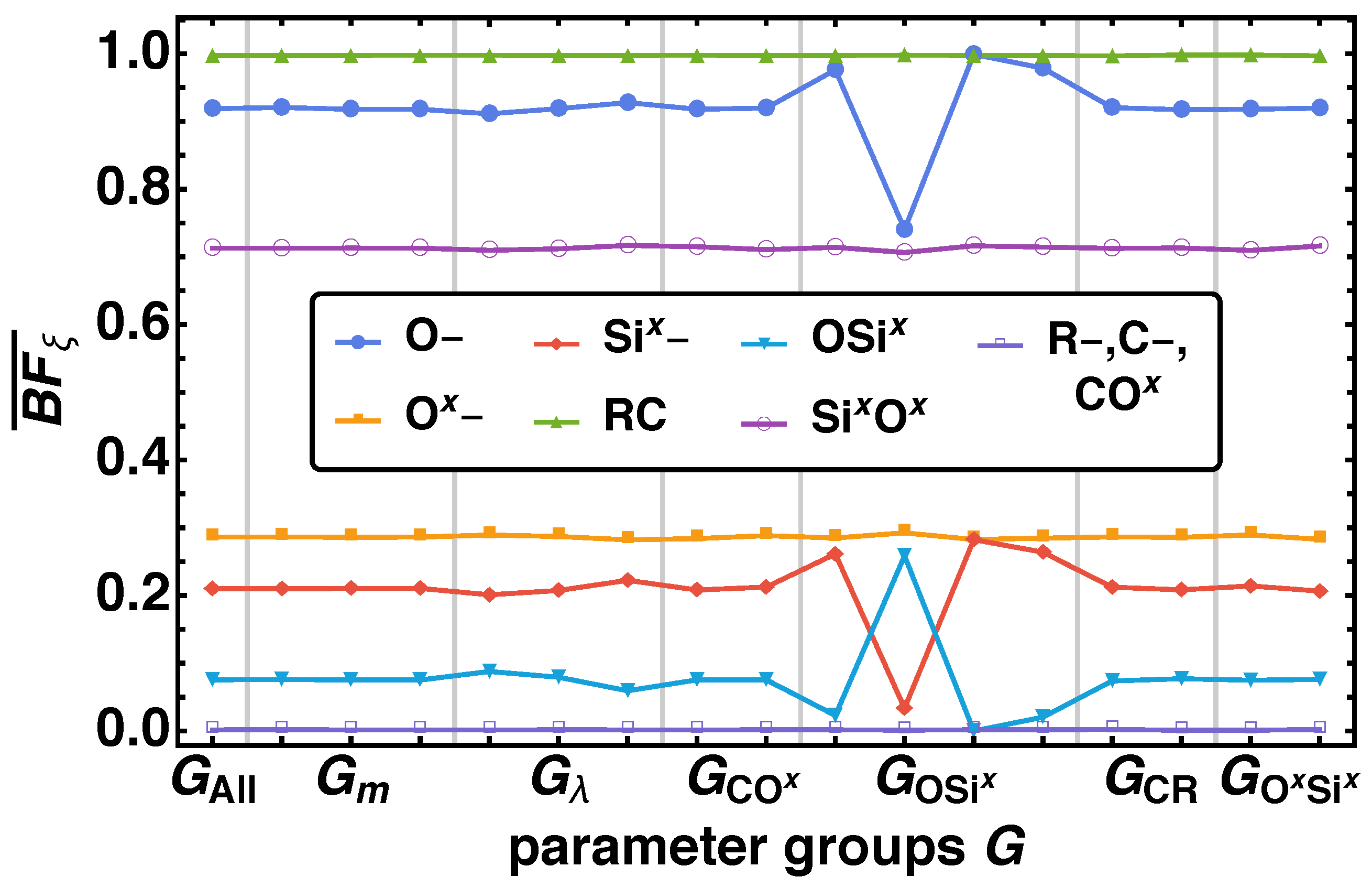
The same behavior is also reflected by the averaged bond fractions over the parameter groups as shown in Figure 6. represents the averaged bond fraction over all parameter combinations. We observe variations of over with from the overall of for O–, Six–, OSix} for two parameter groups and , where the effect of OSix is inverse to O– and Six–. There is a significant variation for , where we can order the parameter groups with decreasing (increasing) order of of O– and Six– (OSix) as , which is also derived from the distributions above. Furthermore, we find the same minor increase (decrease) of for the parameter combinations for O– and Six– (OSix) as from the distributions itself.
3.1.2. Phase Separation
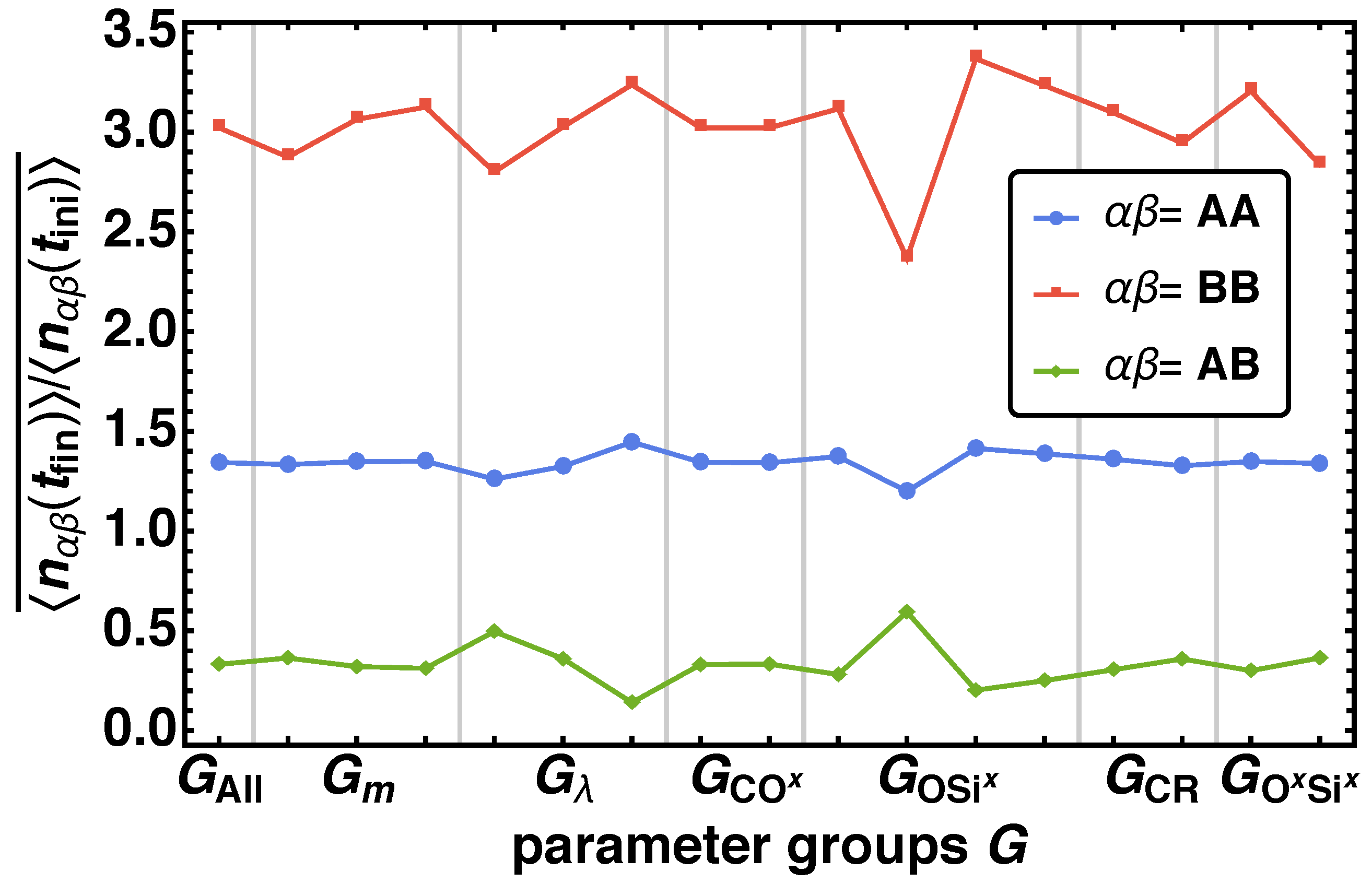
In the next step we investigate the phase separation behavior of the reaction mechanism depending on . Again, for each parameter combination we obtain one value respectively for the mean nearest-neighbor contacts with being the bead type combinations AA, AB, and BB. We determine the averaged mean nearest-neighbor contacts as the arithmetic mean of all values that belong to the parameter combination . In Figure 7 over the parameter groups (see Table 3) are depict. We observe a more complex behavior for than for (compare Figure 6). Again a significant change of for and is found. Additionally, deviations for , , and for BB in major and for ABin minor occurrence can be identified. We find that with increasing m decreasing and the relative number mean nearest-neighbor contacts increases, whereas the effect is inverted for AB. This means that the reduced movability and low network formation reactions hinder the formation of clusters, indicated by a high number of nearest neighbor contact.
From the above analysis of the time development of the reaction process we can conclude that if highly interweaved material with high internal connectivity and no phase separation is need, the twin monomers need to fulfill two important features: A and B should be as miscible as possible ( low) and the movability should be low, while one of the connecting bonds has to have a high activation energy () to compensate phase separation and the corresponding formation of larger cluster.
3.2. Analysis of the Model Parameters on the Structure
In the following, we present the results for the structure properties of the overall material A∪B, as well as for the subsystems A and B. We analyze the specific surface area , the local porosity distribution , the percolation probability , and the percolation fraction with A,B,A∪B}. and the RDF with AA, BB}. As in the previous section, next to the quantities itself we also look at the arithmetic means , i.e., called averaged values in the following, over , if possible.
3.2.1. Bulk Porosity and Specific Surface Area
In Section 2.4 the bulk porosities for our system are given as , , and . Looking at the specific surface areas for we find significant changes of the averaged relative specific surface area . In Figure 8 the averaged relative specific surface areas are given over the parameter groups . In the case of A∪B the strongest influence factor is the attraction parameter , where one observes a decrease of with increasing larger . For and a minimal change in is observable. These effects are magnified for the subsystems A and B. We find an increasing for the parameter groups in the order , where the difference between and the other three groups is in same order as between and . Additionally, we find a secondary effect for the parameter groups and . There an increase of for A, B} for decreasing m and increasing values of and is recognized.
Similar to the bond fraction, and nearest-neighbor analysis we find that nanoporous material with a high specific surface area are obtained, when the twin monomer is designed of components A and B that are are miscible (low ) and the energy barrier of the final connecting bond is high (). Furthermore, a low movability (low m) and a prefered and fast bond formation between identical bead types (high and ) support a high specific surface area of the material.
3.2.2. Radial Distribution Function
The analysis of the RDF , i.e., per each parameter combination there is one resulting RDF, exhibited that the influence of is neglectable and an increase of leads to a minor increase of and of . The main effects are observed for the parameter groups (a)-b)), (c)-d)), and (e)-f)), as depicted in Figure 9. Here, we present the arithmetic mean RDF of all RDFs per parameter combinations that belong to the (thick colored line), as well as the minimum (lowest thin colored line) and maximum (highest thin colored line) out of the corresponding parameter group . The area between the minimum and the maximum curve is covered by the various parameter combination within each parameter group and colored in the same color. In the left column the results for AA and in the right column for BB are presented. Note, that the corresponding subgroups i of each parameter group are highlighted in different colors. From the plots we find two parameter groups with major variations and one with minor one. The major effects are again observed for and for . With increasing and gets higher and wider by a factor of around 1.5–2 in height and width. For BB additionally we observe that for small values of the maximum is truncated. For a major difference is observed between and with . The distributions for are narrow and spiky with lower maximal values, whereas the distributions of the other three groups are broader with higher values, depending on as well. Note that for the width increases up to a factor of 5, whereas the height increases by factor of 1.5–2. Minor difference is displayed by , where find that with increasing m the RDF primary gets wider (factor around 1.5) and only a minimal increase in height.
3.2.3. Local Porosity Distribution
Alternatively to the RDF, the local porosity distribution is used to characterize the pore structure of the material. In Figure 10 the results for the local porosity distributions for A,B,A∪B} are shown exemplary for at in (a,b), and in (c,d) for the two parameter combinations (I) and (II) given in Equations (9) and (10). Analyzing the distributions depending on K, we observe that in all cases the distributions get localized around . This is accepted, as represents the fluctuations of for K and when follows that [31]. Furthermore, we find that the initial distributions for A,B,A∪B} for (I) and (II) are similar in shape independed of the parameters. This reflects the random initialization of the beads on the lattice. However for the distributions are quite different. For (I) the final distributions is more narrow and peaked (see Figure 10c), whereas for (II) they get wider and flatter (see Figure 10d). As the changing width is an important feature of these distributions we will also analyze the variance of the local porosity distributions, next to their mean values (Figure 11).
The averaged mean values of the local porosity distributions are nearly constant at values of the corresponding bulk porosity (see Figure 11a). The variances however, display the previous findings, i.e., changes depending on the parameter groups and . In Figure 10b the averaged variances are given over the parameter groups (see Table 3). We observe for smaller measurement cells larger the fluctuations. For in the case of A∪B and for for the subsystems the variances goes down to 0, thus only results for are plotted. The observed changes in the variance fit very well with the previous findings. The major impact is obtained by varying and . For all the variance increases for with increasing i and we observe the smallest variance for and the largest for . This means the more attractive the beads the wider gets the distribution and the more clusters of different sizes are found. This effect is enhanced if the final connecting bond has a low energy barrier and beads separate easily. Furthermore, the subsystems A and B show a minor dependency on , and . We find a decrease of for decreasing m or for increasing and , i.e., the less the beads move and the faster the networks are formed the more homogenous are the cluster sizes in the final material.
3.2.4. Percolation
Finally, we investigate the total fraction of percolating measurement cells along different directions d given in Table 2 for different cell sizes K. We find that the obtained structures are fully percolating or not at all in nearly all cases, i.e., for and 0 for . There are two exceptions: A∪B and at small and A, B} and . These two cases are shown in Figure 12a,b. As the effects for are similar, but the magnitude of the effect for is larger, we present here only the results for .
In Figure 12a the averaged total fraction of percolating measurement cells is shown for and A∪B at . We find an overall high value of . The highest value is observed for , i.e., there is nearly always a percolating direction within the material. The second highest are found for any single percolating direction (). Here all three directions are nearly the same, thus there is no biased direction within the material. The lowest value is obtained for a percolation all three directions at the same time, i.e., . Independent of the percolating direction, we find an decreasing for increasing , as the beads form packed clusters that are not necessarily connected to both sides of the measurement cell and thus can not percolate. We find that an enhanced network formation (high value of ) and a low movability of the beads (low value of m), increases . This can be accounted to the high connectivity of identical beads due to the fast network formation or due to the homogeneous distribution of beads, as they can not move too far away from the initial homogeneous distribution. Interestingly, shows here only a minor influence on the percolation for A∪B. In Figure 12b we show for A and B for all K. Here, the case of no percolation in any direction is analyzed. As mentioned above, for , but for the subsystems it is not. Analyzing the general behavior of over K we find that for the bead type A that percolation is restored for system size , whereas for B it already restored for . For both subsystems we find changes in , depending on and , similar to the previous results. With increasing decreases, as the probability of percolation increases. There is a drastic drop of for , as the high connectivity of the beads for this parameter combination typically leads to percolation. This effect is also indicated by the decrease of for increasing . Finally the decrease of with decreasing m is due to the low movability that keeps the beads close to their initial random starting position on the lattice, which enhances the chance of percolation.
4. Summary
The focus of this work was the derivation of a structure on reaction process dependency for twin polymerization and the identification of influencing factors to modify the final morphology to allow an application-oriented adaptation of the final twin polymers. Therefore, we utilized the previously introduced reactive bond fluctuation model for twin polymerization of the typical twin monomer 2,2-spiro[4H-1,3,2-benzodioxasiline]. We kept the reaction mechanism and the basic composition of the twin monomer for our analysis as both can be recovered for many other twin monomers as well. However, we varied all reaction relevant parameters and analyzed their effects on the final morphology. In this context, we investigate various chemical and structural properties, that are directly or indirectly connected with the reaction mechanism, as the bond fractions, the specific surface area, the bulk and the local porosity, percolation effects and the radial distribution function for a wide range of possible parameter combinations.
Our investigations showed that there are four main components that affect the final morphologies; most of all: That are the attraction between the two chemical components (beads), the strength, i.e., activation energy, of the final connecting bond between two different bead types, the probability of identical beads to form bonds and the movability of the beads. The more attractive identical bead types are the more often the beads are bonded and thus the larger and more heterogenous are the clusters sizes of identical beads. Consequently, the specific surface area decreases, the cluster size and number of beads per cluster increases, and the percolation probability decreases. The higher activation energy of the final connecting bond, the longer are the beads of different type connected, and thus, the smaller are the cluster sizes and beads per cluster leading to more homogenous materials. This is also reflected in the percolation property of the obtained materials, as a high connectivity increases the probability to find percolation. The described effects of the strength of the final connecting bond can be enhanced by increasing the probability to form networks between identical bead types. Additionally, we found that the movability influences the structural properties of the material as well. The higher the movability, the larger the cluster sizes and number of beads per clusters, i.e., the material is more heterogenous due to the different cluster sizes and this decreases the percolation probability, however, note that the bond fractions have not been affected by the movability.
Hence, we found a direct dependency of the reaction relevant parameters to structural properties of the final morphology. We were able to deduce direct proportionalities on how to change the underlying components to design certain effects, i.e., a high specific surface area or homogeneous cluster sizes, within the material. At this point it is now of special interest to analyze the already known class of twin monomers with respect to the above-mentioned main components that affect the morphology and to compare the resulting findings with the properties of the used 2,2-spiro[4H-1,3,2-benzodioxasiline]. So we will be able to classify the twin monomers within our parameter groups and to check our prediction on the real materials.
Author Contributions
Both authors contributed equally to the publication: conceptualization, methodology, software, validation, formal analysis, investigation: C.H., J.P.; writing, visualization, supervision, project administration, funding acquisition: J.P.
Funding
This research was funded by the German Research Foundation/DFG in the framework of the DFG Forschergruppe (FOR) 1497, grant number PR 1580/1-1 and the publication costs of this article were funded by the German Research Foundation/DFG -392676956 and the Technische Universität Chemnitz in the funding program Open Access Publishing.
Conflicts of Interest
The authors declare no conflict of interest.
Abbreviations
The following abbreviations are used in this manuscript:
| BFM | bond fluctuation model |
| rBFM | reactive bond fluctuation model |
| RDF | radial distribution function |
| nMC, rMC | non-reactive Monte Carlo, reactive Monte Carlo |
References
- Higgins, B.A.; Brittain, W.J. Polycarbonate carbon nanofiber composites. Eur. Polym. J. 2005, 41, 889–893. [Google Scholar] [CrossRef]
- Chemtob, A.; Belon, C.; Croutxé-Barghorn, C.; Rigolet, S.; Vidal, L.; Brendlé, J.; Mandle, J.; Blanchard, N. Tandem Cationic and Sol–Gel Photopolymerizations of a Vinyl Ether Alkoxysilane. Polym. Eng. Sci. 2011, 51, 1466–1475. [Google Scholar] [CrossRef]
- Ni, L.; Moreau, N.; Chemtob, A.; Croutxé-Barghorn, C. Organic–inorganic tandem route to polymer nanocomposites: kinetic products versus thermodynamic products. J. Sol-Gel Sci. Technol. 2012, 64, 500–509. [Google Scholar] [CrossRef]
- Rodrígez-Tobías, H.; Morales, G.; Rodríguez-Fernández, O.; Acuña, P. Mechanical and UV-Shielding Properties of In Situ Synthesized Poly(acrylonitrile-butadiene-styrene)/Zinc Oxide Nanocomposites. J. Appl. Polym. Sci. 2013, 127, 4708–4718. [Google Scholar] [CrossRef]
- Wang, Y.; Jabarin, S.A. Novel preparation method for enhancing nanoparticle dispersion and barrier properties of poly(ethylene terephthalate) and poly(m-xylylene adipamide). J. Appl. Polym. Sci. 2013, 129, 1455–1465. [Google Scholar] [CrossRef]
- Ebert, T.; Seifert, A.; Spange, S. Twin polymerization—A new principle for hybrid material synthesis. Macromol. Rapid Commun. 2015, 36, 1623–1639. [Google Scholar] [CrossRef]
- Grund, S.; Kempe, P.; Baumann, G.; Seifert, A.; Spange, S. Zwillingspolymerisation: Ein Weg zur Synthese von Nanokompositen. Angew. Chem. 2007, 119, 636–640. [Google Scholar] [CrossRef]
- Spange, S.; Kempe, P.; Seifert, A.; Auer, A.A.; Ecorchard, P.; Lang, H.; Falke, M.; Hietschold, M.; Pohlers, A.; Hoyer, W.; et al. Nanocomposites with Sturcture Domains of 0.5 to 3 nm by Polymerization of Silicon Spiro Compounds. Angew. Chem. Int. Ed. 2009, 48, 8254–8258. [Google Scholar] [CrossRef]
- Huster, C.; Nagel, K.; Spange, S.; Prehl, J. A reactive bond fluctuation model (rBFM) for twin polymerization: Comparison of simulated morphologies with experimental data. Chem. Phys. Lett. 2018, 713, 145–148. [Google Scholar] [CrossRef]
- Spange, S.; Grund, S. Nanostructured Organic-Inorganic Composite Materials by Twin Polymerization of Hybrid Monomers. Adv. Mater. 2009, 21, 2111–2116. [Google Scholar] [CrossRef]
- Brückner, J.; Thieme, S.; Böttger-Hiller, F.; Bauer, I.; Grossmann, H.T.; Strubel, P.; Althues, H.; Spange, S.; Kaskel, S. Carbon-Based Anodes for Lithium Sulfur Full Cells with High Cycle Stability. Adv. Funct. Mater. 2014, 24, 1284–1289. [Google Scholar] [CrossRef]
- Kitschke, P.; Walter, M.; Rüffer, T.; Seifert, A.; Speck, F.; Seyller, T.; Spange, S.; Lang, H.; Auer, A.A.; Kovalenko, M.V.; Mehring, M. Porous Ge@C materials via twin polymerization of germanium(II) salicyl alcoholates for Li-ion batteries. J. Mater. Chem. A 2016, 4, 2705–2719. [Google Scholar] [CrossRef]
- Spange, S.; Mehring, M. (Eds.) Twin Polymerization—New Strategy for Hybrid Materials; DeGruyter: Berlin/Boston, Germany, 2018. [Google Scholar]
- Auer, A.A.; Richter, A.; Berezkin, A.V.; Guseva, D.V.; Spange, S. Theoretical Study of Twin Polymerization—From Chemical Reactivity to Structure Formation. Macromol. Theory Simul. 2012, 21, 615–628. [Google Scholar] [CrossRef]
- Tchernook, I.; Prehl, J.; Friedrich, J. Quantum chemical investigation of the counter anion in the acid catalyzed initiation of 2,2’-spirobi[4H-1,3,2-benzodioxasiline] polymerization. Polymer 2015, 60, 241–251. [Google Scholar] [CrossRef]
- Schönfelder, T.; Friedrich, J.; Prehl, J.; Seeger, S.; Spange, S.; Hoffmann, K.H. Reactive force field for electrophilic substitution at an aromatic system in twin polymerization. Chem. Phys. 2014, 440, 119–126. [Google Scholar] [CrossRef]
- Prehl, J.; Schönfelder, T.; Friedrich, J.; Hoffmann, K.H. Site Dependent Atom Type ReaxFF for the Proton-Catalyzed Twin Polymerization. J. Phys. Chem. C 2017, 121, 15984–15992. [Google Scholar] [CrossRef]
- Hoffmann, K.H.; Prehl, J. Modeling the structure formation process of twin polymerization. Reac. Kinet. Mech. Cat. 2018, 123, 367–383. [Google Scholar] [CrossRef]
- Fiedler, B.; Friedrich, J.; Prehl, J. Modeling and simulation of nanostructure formation of TP. In Twin Polymerization—New Strategy for Hybrid Materials Synthesis, 1st ed.; Stefan, S., Mehring, M., Eds.; Walter de Gruyter: Berlin, Germany, 2018; Chapter 3.3; pp. 135–166. [Google Scholar]
- Carmesin, I.; Kremer, K. The Bond Fluctuation Method: A new effective algorithm for the dynamics of polymers in all spatial dimensions. Macromolecules 1988, 21, 2819–2823. [Google Scholar] [CrossRef]
- Shaffer, J.S. Effects of chain topology on polymer dynamics: Bulk melts. J. Comput. Phys. 1994, 101, 4205–4213. [Google Scholar] [CrossRef]
- Subramanian, G.; Shanbhag, S. On the relationship between two popular lattice models for polymer melts. J. Chem. Phys. 2008, 129. [Google Scholar] [CrossRef]
- Paul, W.; Pistoor, N. A mapping of realistic onto abstract polymer models and an application to two bisphenol polycarbonates. Macromolecules 1994, 27, 1249–1255. [Google Scholar] [CrossRef]
- Tries, V.; Paul, W.; Baschnagle, J.; Binder, K. Modeling polyethylene with the bond fluctuation model. J. Chem. Phys. 1997, 106, 738–748. [Google Scholar] [CrossRef]
- Malik, R.; Hall, C.K.; Genzer, J. Phase Separation Dynamics for a Polymer Blend Compatibilized by Protein-like Copolymers: A Monte Carlo Simulation. Macromolecules 2011, 44, 8284–8293. [Google Scholar] [CrossRef]
- Rubio, A.M.; Storey, M.; Lodge, J.F.M.; Freire, J.J. Dynamics of Bond-Fluctuation Model Chains in Good and Theta Solvents. Macromol. Theory Simul. 2002, 11, 171–183. [Google Scholar] [CrossRef]
- Nakagawa, N.; Maeda, S.; Ishii, S.; Ohno, K. A Monte Carlo Simulation of the Formation of Micelles in a Ternary System of Water, Oil and Amphiphilic Polymers. Mat. Trans. 2007, 48, 653–657. [Google Scholar] [CrossRef] [Green Version]
- Müller, M. Miscibility behavior and single chain properties in polymer blends: a bond fluctuation model study. Macromol. Theory Simul. 1999, 8, 343–374. [Google Scholar] [CrossRef]
- Kempe, P.; Löschner, T.; Adner, D.; Spange, S. Selective ring opening of 4H-1,3,2-benzodioxasiline twin monomers. New J. Chem. 2011, 35, 2735–2739. [Google Scholar] [CrossRef]
- Kitschke, P.; Auer, A.A.; Löschner, T.; Seifert, A.; Spange, S.; Rüffer, T.; Lang, H.; Mehring, M. Microporous Carbon and Mesoporous Silica by Use of Twin Polymerization: An Integrated Experimental and Theoretical Approach to Precursor Reactivity. ChemPlusChem 2014, 79, 1009–1023. [Google Scholar] [CrossRef]
- Biswal, B.; Manwart, C.; Hilfer, R. Three-Dimensional Local Porosity Analysis of Porous Media. Physica A 1998, 255, 221–241. [Google Scholar] [CrossRef]
Figure 1.
The chemical structure of the typical twin monomer 2,2-spiro[4H-1,3,2-benzodioxasiline] is shown in (a), and its reactive bond fluctuation (rBFM) representation in 2D in (b). It is represented by two bead types (A,B) and five different reaction centers (O,C,R,Ox,Six, with ) as illustrated in (c,d). In (d) all possible states of the reaction centers and all possible bond vector types are given in an exemplary 2D-cutout of the cubic lattice. A corresponding 3D representation is given in Figure 2. Reaction centers with a solid square are bonded, with a dashed square are non-bonded and with darker filling are blocked. Note that to make it easier to differentiate between the reaction centers that are all placed in the center of the beads, here they are plotted next to each other.

Figure 2.
Exemplary snapshots of a reduced 3D cubical lattice of reduced size at (a) and (b) for the parameter combination (I) (see Equation (9)) and two corresponding cutouts of size (c): ; (d): ) that are magnified to show the actual existing bond vectors. The colors are chosen in analogy to Figure 1. In (c) only twin monomer structures are observed (see Figure 1b). As over reaction time bonds may cleave and form, a final structure emerge as depict in (d), where a small organic (gray gray) and inorganic (red bonds) network emerge. Note that some initial bonds (green) may survive till the end. The origin of both sub cubes is at position within the large 3D cubes. Note that to make it easier to differentiate between the bond vector types that are connected to the center of the beads, here they are plotted next to each other.

Figure 3.
The acid catalyzed reaction scheme of the typical twin monomer 2,2-spiro[4H-1,3,2-benzodioxasiline] (1) is shown. 1twin polymerizes to a phenolic resin (2) and a silica network (3).
Figure 3.
The acid catalyzed reaction scheme of the typical twin monomer 2,2-spiro[4H-1,3,2-benzodioxasiline] (1) is shown. 1twin polymerizes to a phenolic resin (2) and a silica network (3).

Figure 4.
The time development of the bond fractions of all bond vector types COx, OSix, CR, SixOx} in (a,c) and of the non-bonded reaction centers C–, O–, R–, Ox–, Six–} in (b,d) are given for the two exemplary parameter combinations (I) and (II) (a–d). Note that in (d) the curve for C– is plotted thicker, as it falls on top of the curve for R– and Ox–.

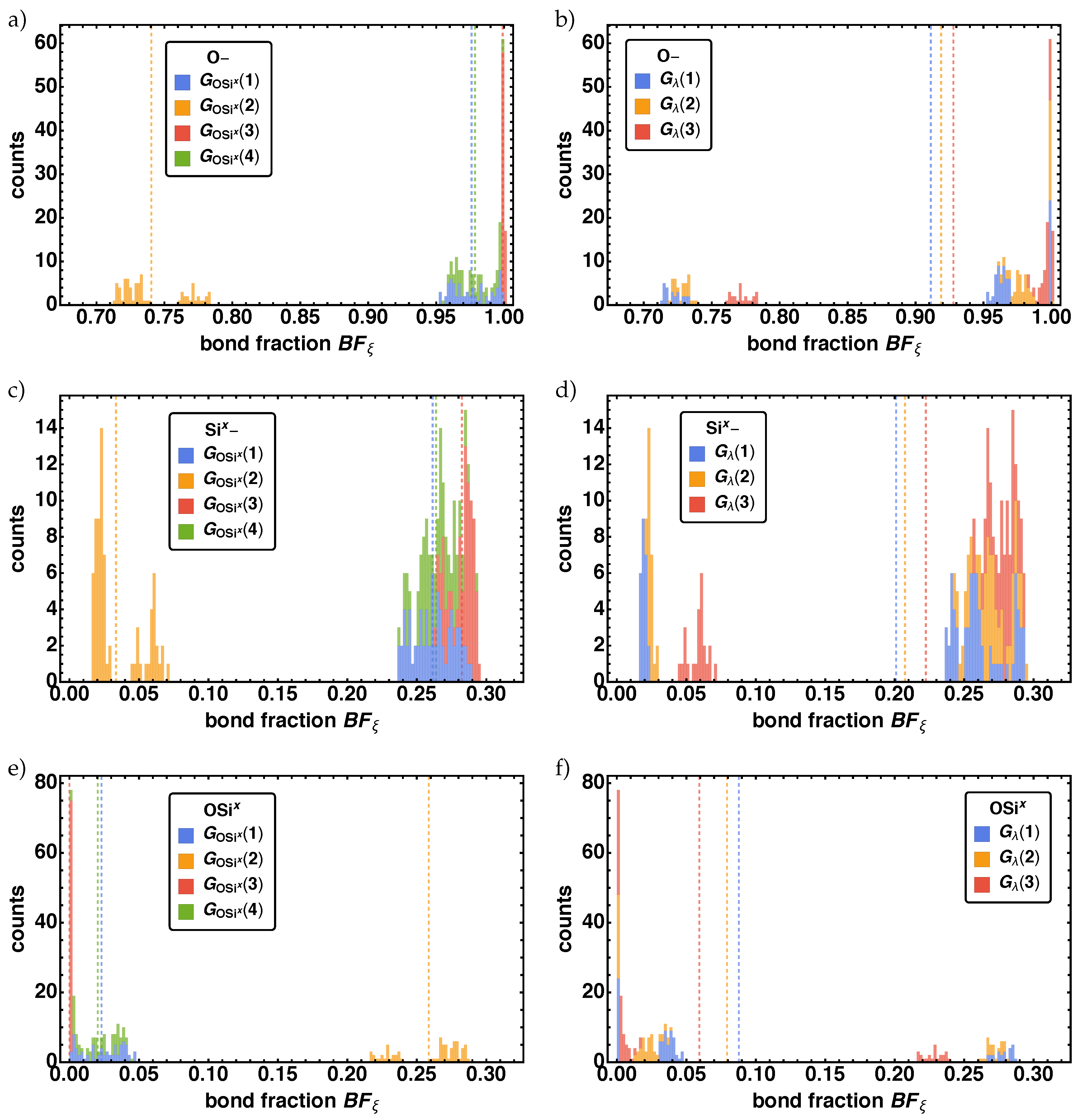
Figure 5.
Distributions of the bond fractions at for the non-bonded reactions centers O–, Six–} in (a–d), and the bond vector type OSix in (e,f) for the two parameter combinations (left column) and (right column).
Figure 5.
Distributions of the bond fractions at for the non-bonded reactions centers O–, Six–} in (a–d), and the bond vector type OSix in (e,f) for the two parameter combinations (left column) and (right column).

Figure 6.
Averaged bond fractions at for all non-bonded reaction center O–, C–, R–, Ox–, Six–} and bond vector types COx, CR, OSix, SixOx} over the parameter groups specified in Table 3.
Figure 6.
Averaged bond fractions at for all non-bonded reaction center O–, C–, R–, Ox–, Six–} and bond vector types COx, CR, OSix, SixOx} over the parameter groups specified in Table 3.

Figure 7.
Averaged mean nearest-neighbor contacts for all parameter groups for the bead type combinations AA, AB, BB}.
Figure 7.
Averaged mean nearest-neighbor contacts for all parameter groups for the bead type combinations AA, AB, BB}.

Figure 8.
The averaged relative specific surface area is given for the parameter groups (see Table 3).
Figure 8.
The averaged relative specific surface area is given for the parameter groups (see Table 3).

Figure 9.
The arithmetic mean, i.e., averaged (thick colored line), the minimum (lowest thin colored line) and the maximum (highest thin colored line) radial distribution function over radial distance r are given for ba = fAA, BBg in (a,c,e) and (b,d,f) and for the parameter groups , and in (a,b), (c,d), and (e,f). Each subgroup i is highlighted with a different color.

Figure 10.
The local porosity distributions for and A, B, A∪B} are given over the local porosity for the two parameter combinations (I) and (II). In (a,b) the initial and in (c,d) the final distributions are shown.
Figure 10.
The local porosity distributions for and A, B, A∪B} are given over the local porosity for the two parameter combinations (I) and (II). In (a,b) the initial and in (c,d) the final distributions are shown.

Figure 11.
In a) the averaged mean values of the local porosity distribution and in b) the averaged variances for different lengths of the measurement cells for A, B, A∪B} are shown over the parameter groups . Note that for all variances are 0 and thus are not shown here.
Figure 11.
In a) the averaged mean values of the local porosity distribution and in b) the averaged variances for different lengths of the measurement cells for A, B, A∪B} are shown over the parameter groups . Note that for all variances are 0 and thus are not shown here.

Figure 12.
The averaged total fraction of percolating measurement cells with and 1 are given over the parameter groups (see Table 3). The results are shown in (a) for =A∪B, , and , whereas in (b) for A, B} and .
Figure 12.
The averaged total fraction of percolating measurement cells with and 1 are given over the parameter groups (see Table 3). The results are shown in (a) for =A∪B, , and , whereas in (b) for A, B} and .


Table 1.
All varied model parameters and corresponding analyzed values of the reactive bond fluctuation model are listed.
Table 1.
All varied model parameters and corresponding analyzed values of the reactive bond fluctuation model are listed.
| Model Parameter (Variable) | Symbol | Analyzed Values |
|---|---|---|
| COx cleavage | ||
| OSix cleavage | ||
| OSix formation | ||
| CR formation | ||
| SixOx formation | ||
| ratio rMCS/nMCS | m | |
| attraction parameter |
Table 2.
Investigated percolation directions d. With index the corresponding space directions are indicated. Index represent percolation in all directions at the same time, at least one direction, and stands for no percolation at all.
Table 2.
Investigated percolation directions d. With index the corresponding space directions are indicated. Index represent percolation in all directions at the same time, at least one direction, and stands for no percolation at all.
| Index d | Meaning | Index d | Meaning |
|---|---|---|---|
| x | x-direction | 3 | -direction |
| y | y-direction | c | -direction |
| z | z-direction | 0 | -direction |
Table 3.
17 parameter groups are defined, where typically one parameter value is fixed. The corresponding parameter values for each group are given in first column and the short notation in the second.
Table 3.
17 parameter groups are defined, where typically one parameter value is fixed. The corresponding parameter values for each group are given in first column and the short notation in the second.
| Model Parameter | Notation | Model Parameter | Notation |
|---|---|---|---|
| average over all | |||
© 2019 by the authors. Licensee MDPI, Basel, Switzerland. This article is an open access article distributed under the terms and conditions of the Creative Commons Attribution (CC BY) license (http://creativecommons.org/licenses/by/4.0/).
Share and Cite
MDPI and ACS Style
Prehl, J.; Huster, C. Morphology on Reaction Mechanism Dependency for Twin Polymerization. Polymers 2019, 11, 878. https://doi.org/10.3390/polym11050878
AMA Style
Prehl J, Huster C. Morphology on Reaction Mechanism Dependency for Twin Polymerization. Polymers. 2019; 11(5):878. https://doi.org/10.3390/polym11050878
Chicago/Turabian StylePrehl, Janett, and Constantin Huster. 2019. "Morphology on Reaction Mechanism Dependency for Twin Polymerization" Polymers 11, no. 5: 878. https://doi.org/10.3390/polym11050878
Note that from the first issue of 2016, this journal uses article numbers instead of page numbers. See further details here.