Review

Hybrid Lattice Particle Modelling Approach for Polymeric Materials Subject to High Strain Rate Loads

1
Department of Civil Engineering, University of Mississippi, University, MS 38677, USA
2
Department of Mechanical and Industrial Engineering, University of Illinois at Urbana-Champaign, Urbana, IL 61801, USA
3
Department of Mechanical Engineering, McGill University, Montreal, H3A 2K6, Canada
*
Author to whom correspondence should be addressed.
Polymers 2010, 2(1), 3-30; https://doi.org/10.3390/polym2010003
Submission received: 25 February 2010 / Revised: 23 March 2010 / Accepted: 23 March 2010 / Published: 25 March 2010
(This article belongs to the Special Issue Novel Stimuli-Responsive (co)Polymers)

Abstract

:
Hybrid Lattice Particle modelling (HLPM) is an innovative particular dynamics approach that is established based on a combination of the particle modelling (PM) technique together with the conventional lattice modelling (LM) theory. It is developed for the purpose of simulating the dynamic fragmentation of solids under high strain rate loadings at macroscales with a varying Poisson's ratio. HLPM is conceptually illustrated by fully dynamic particles (or “quasi-particles”) placed at the nodes of a lattice network without explicitly considering their geometric size. The interaction potentials among the particles can employ either linear (quadratic) or nonlinear (Leonard-Jones or strain rate dependent polynomial) type as the axial/angular linkage. The defined spring constants are then mapped into lattice system, which are in turn matched with the material’s continuum-level elastic moduli, strength, Poisson's ratio and mass density. As an accurate dynamic fracture solver of materials, HLPM has its unique advantages over the other numerical techniques which are mainly characterized as easy preparation of inputs, high computation efficiency, ability of post-fracture simulation and a multiscale model, etc., This paper is to review the successful HLPM studies of dynamic fragmentation of polymeric materials with good accuracy. Polymeric materials, including nylon 6-6, vinyl ester and epoxy, are accounted for under the loading conditions of tension, indentation and punctuation. In addition, HLPM of wave propagation and wave induced fracture study is also reviewed.

1. Introduction

Polymeric materials, e.g., nylon 6-6, vinyl ester and epoxy, etc., are of lightweight, tough, corrosion resistant [1], and can be easily glued into complex components with various functions and features. These desirable features have offered polymeric materials a broad application areas, e.g., of building and construction, manufacture, transportation, furniture, electronics and machinery, etc. Structural polymers and polymer composites are exciting new materials and are anticipated to be a replacement material for conventional engineering materials such as wood, stone, glass and metal. This is without doubt a significant and exciting perspective nowadays when human beings are facing a rapid shortage of natural resources.
Since polymeric materials are being more and more widely used as structural components in engineering fields, especially those with the high strain rate loads (impact, blasting, crush, collapse, high speed puncture/penetration, etc.), the fundamental research work on dynamic and fracture characteristics of polymeric materials is of a remarkable importance [2,3,4,5,6].
Dynamic fracture is a complex and multi-scale physical phenomenon. From the microscopic point of view, fracturing is a process that material becomes separated due to the successive breakage of atomic bonds. Since the intrinsic strength properties at molecular structure level are available, molecular dynamics (MD) analysis has been attempted at the nano scale. However, although MD simulation has benefitted from the rapid development of computing power and is becoming increasingly popular, the present state of computer technology is still far from being able to meet the demands of the macroscopic tasks. For example, we currently still cannot simulate a 1 × 1 × 1 cm3 cubic copper body at atomic level because the body consists of 1024 copper atoms, a number so large that no computer in the world can handle it. The second difficulty is its incapability in reaching the practical time scales. For instance, the laboratory dynamic fracture experiments generally last in microseconds (1 microsecond = 10−6 s), while the MD model time steps are typically in the nano (10−9) or pico (10−12) second range. As such, MD is limited to a narrow range of solving nano- to micrometer scale problems. For this reason, numerical tools for the modelling of dynamic fracture at macroscopic level are needed.
Static or quasi-static models have existed for several decades and successfully been used for micromechanics and macro-mechanics structure analysis. However, they fail to become a tool for dynamic fracture of solids. The reason arises from the fundamental differences between static (or quasi-static) and dynamic deformation. In a quasi-static deformation, at any time, a situation of static equilibrium holds, which implies that any element in the material body has a summation of forces acting on it close to zero. In contrast, in a dynamic deformation, when a high strain rate loading is applied to the boundary of the body, the stress propagates, that is, the stress has to travel through the body. This is called wave propagation. Thus, dynamic deformation often involves wave propagation. Consequently, a sequence of states of equilibrium defined by the well-known equations of mechanics of materials (summation of forces equal to zero, summation of moments equal to zero; compatibility of strain; constitutive relations, etc.) are no longer valid.
The current numerical methods for dynamic fracture simulation at macroscopic level can be classified into two categories—continuum mechanics based models (CMBM for short) and discrete element based models (DEBM for short).
Current CMBMs, e.g., a finite element method (FEM), are well known to limit the fracture/fragmentation predictions. The FEM regards material as one continuum media, and the global element assembly technique employed by FEM follows the compatibility condition [7] which states that the interior nodes still remain connected after deformation, i.e., must have the same nodal displacement; hence, once the continuity of material is broken due to the presence of fracture or fragmentation, re-meshing is required to distinguish the interior and boundary nodes in need of correct element assembly at a new evolving stage of geometry for the next cycle of computation. When a material body is subject to extreme loadings, unexpected fragments are often produced. Herein, this offers FEM an extreme challenge in technique to deal with the dynamic re-meshing, and causes the computation highly expensive. Although FEM has constantly been developed to meet such requirements and several re-meshing techniques (i.e., Lagrange, Euler and Arbitrary Lagrange Euler) [8], and some hybrid sophisticated methods [9] have been well established and embedded into FEM, it still cannot well and easily predict multi-cracks of materials, let alone the fragmentation problems. Figure 1 displays the comparison of using FEM and smoothed particle hydrodynamics (SPH), a discrete element based method (DEBM) [10], in simulating material penetration [8]. It is seen that, although the FEM employs powerful re-meshing techniques, the fragmentation of material is still not able to be predicted. Meanwhile, it illustrates that the DEBM is superior to the CMBM in dealing with the fragmentation of materials. As such, discrete element based methods (DEBM), e.g., SPH, particle flow code (PFC) [11], applied element method [12], particle modelling (PM) [13,14,15], and the further developed hybrid lattice particle modelling (HLPM) [16], etc., have been established at a macroscopic level. DEBM is established based on treating material as an assembly of mass particles. The constitutive equations are assigned to define the interactions among the discrete neighboring particles. Consequently, DEBM does not suffer from either the mesh tangling problem encountered when using Lagrangian mesh or the material flux conservation problem when using Eulerian mesh. This leads to DEBM unique robustness to solve the ‘discontinuity of material’ problems. Due to the irreplaceable superiority of DEBM to CMBM in solving the fragmentation of materials, the 'discrete material' concept is becoming more and more widely accepted by engineering fields, and the market for DEBM applications is increasingly growing. This gives rise to a more prosperous DEBM modelling research in this decade. Meanwhile, there are newly developed models that couple DEBM with CMBM, e.g., particle finite element method (PFEM) [17] and material point method (MPM) [18], etc., in which the deformation is solved using CMBM while the fracture/fragmentation relies on DEBM. Since DEBM is the core in fracture/fragmentation simulations, to improve/develop techniques of various DEBMs is of significant importance and value.
All the current DEBMs can be classified into two categories: mesh free (or meshless) and lattice particle models. For example, SPH, PFC and their inherited subclass of methods are mesh free models since the computations do not rely on a meshing system. In contrast, the confinement-shear lattice model (CSLM for short) [19,20], PM and HLPM are lattice particle models since the simulations are carried out on a lattice structure. In lattice particle models, the neighborhood of each particle needs to be pre-defined, and the consequent evolution of deformation, fracture or fragmentation at each fracturing stage can be readily identified and predicted with the pre-defined neighborhood.
Figure 1. A material impact simulation by using FEM accounting for different re-meshing skills, Lagrange, Euler and Arbitrary Lagrange Euler (ALE), and smoothed particle hydrodynamics (SPH) [8].
Polymers 02 00003 g001
In the domain of meshless models, PFC and SPH are the two most notable techniques. Many new developed meshless models and the according hybrid CMBM-DEBM techniques originate from these two models. However, viewing from the current technological status of meshfree models, they are, in general, far less complete in technique. This imperfection partially arises from the fact that the dynamic fracture mechanics model study is still at a quite fundamental stage, and partially from inherent limits of each individual model which can be summarized as follows:
(1)
In PFC and its inherited subclass of developed methods, each particle's size is physically accounted for, e.g., circular discs or spheres used for 2D or 3D, respectively. In summary, three disadvantages of PFC are obvious: (i) particle packing causes porosity of material. It is obviously not suitable for compact/condense materials; (ii) material's Poisson's ratio cannot be related to the pattern of the packed particles; and (iii) expensive computation is spent in keeping track of the instantaneous contact positions and the evolving geometry of all elements.
(2)
In SPH, a kernel density function, or weight function, is employed to define each particle's reaction domain, and continuum constitutive equations are then applied to particles within the domain. In recent years, several new techniques have been established to modify the kernel function to improve the computation accuracy. These new techniques are element-free Galerkin method (EFGM) [21], reproducing kernel particle method (RKPM) [22] and partition of unity method (PUM) [23,24]. As was mentioned by Belytschko [25], in most cases, these approaches are identical. On the whole, SPH is currently still at an immature status in technique and needs considerable improvement so as to overcome the two major limits of (i) that the SPH was developed with in mind more fluid modelling than solid modelling. However, for solids, pre-fracture particle-particle interactions are different from the failed, while they are conserved in fluids. For instance, a blend of two separate parts of fluid follows the same constitutive equations, whereas a mixture of two separate solid parts does not follows the same interactive formulas as one integrated body applies. Consequently, post-fracture interaction of solids cannot be readily traced since the kernel density function cannot distinguish if the particles are pre-fractured or to be failed; and (ii) high complexity in computation. SPH is a time-consuming technique while the inherited meshless derivatives are even more expensive [25].
Compared with the meshless techniques, dynamic lattice techniques are currently far less popular and consequently less developed. However, they show promises as robust tools due to some unique properties.
Cusatis's confinement-shear lattice model (CSLM) [19,20] conducted on an irregular and randomly generated meshing system, Delaunay triangulation mesh, has demonstrated its ability in fracture predictions. However, the CSLM validations are found to have been accomplished so far with merely quasi-static cases, ignoring the inertia term, rather than dealing with high strain rate loadings. Further, the complex meshing technique in the model undoubtedly leads to high expenses in computations and limits it to post-fracture applications. Furthermore, it needs to be especially pointed out here that, since the location of the stress or pressure gradient in dynamic simulations is dependent on time and space, spurious wave reflection may arise from this irregular mesh system due to the presence of different limits to the wavelength generated by the irregular nodal spacing [21,27]. To prevent this problem, no less than 10% gradual difference between neighboring grid should be obeyed [28].
Hybrid lattice particle modelling (HLPM) [16] has been proposed to combine the strengths of both the lattice model (LM) [26] and PM [14], in which the interaction potentials can be described by employing either linear (quadratic) or nonlinear (Leonard-Jones or strain rate dependent polynomial) type to the axial/angular linkage, see Figure 2. The defined spring constants are then mapped into the lattice system, which are in turn matched with the material’s continuum-level elastic moduli, strength and Poisson's ratio. Axial (α-model), axial-angular (α-β-model) and ‘triple honeycomb lattice’ method (α-β-γ-model) models have been developed together with considering triangular lattice and various particle-particle interactions (nearest and two-layer neighboring), shown in Figure 3. The theoretical derivations of different considerations associated with the material's properties have been well addressed by Wang et al. [16].
The HLPM can readily simulate dynamic behaviors/fragmentation of materials at macro-scales with a varying Poisson’s ratio. For instance, assigning the same α and β to the axial and angular springs in 2D works for the Poisson's ratio ranging from (–1, 1/3] [16]; whereasα-β-γ-model works for the Poisson’s ratio ranging from [1/3, 1) [26]. Moreover, the HLPM can also efficiently solve a 'mesh bias' and 'lattice interpenetration problem that the conventional LM is plagued with [13]. The principle of HLPM can be described as follows: the particle-particle interaction is derived from lattice modelling (LM) theory whereas the computational scheme follows the particle modelling (PM) technique. Once the translational strength is exceeded, the spring is broken and a fracture is created. The strength of HLPM over the traditional LM and PM is summarized and compared in Table 1.
Table 1. Comparison of the lattice model (LM), the particle model (PM), and the hybrid lattice particle model (HLPM).
Lattice Model (LM)Particle Model (PM)Hybrid Lattice Particle Model (HLPM)
Particle interactionspring (axial/angular), beam, etc.Leonard-Jones potential (axial only)spring (axial/angular) mimicking the Leonard-Jones potential
Interaction neighborhoodnot limited to nearest neighbornearest neighbor onlynot limited to nearest neighbor
Mesh systemsmall deformationlarge deformationlarge deformation
Poisson’s ratioflexiblefixedflexible
Time processstaticdynamic based on Newton’s second lawdynamic based on Newton’s second law
Force-displacement relationDisplacement (strain) interpreted from force (stress)Force interpreted from displacement (distance between particles)Force interpreted from displacement (distance between particles)
Figure 2. Force interaction types of HLPM: (a) Lennard–Jones, (b) linear, (c) strain-rate dependant polynomial.
Polymers 02 00003 g002
Figure 3. Interaction schemes in HLPM: (a) nearest neighboring axial interaction; (b) two-layer axial interaction (c) α-β model in equal-lateral triangular lattice structure; and (d) α-β-γ model in triangular lattice structure.
Polymers 02 00003 g003
The advantages of HLPM over the other existing DEBMs can be summarized as follows:
(1)
Easy for the determination of input parameters. Five conservative/equivalent rules (mass, potential energy, Young’s modulus, tensile/compressive strength and Poisson's ratio) are required to determine the material's properties for the input datasheet.
(2)
Easy for implementation and high computation efficiency. Since the physical size of each particle is ignored rather than its equivalent mass, the algorithm of coding a HLPM computation is fairly easy; meanwhile, since no computation is spent in keeping track of the instantaneous contact positions and the evolving geometry of all elements, the HLPM computing cost is greatly reduced.
(3)
Easy for tracing the post-fracture interactions. In HLPM, a pre-defined neighborhood in a lattice structure represents the integrated and non-fractured body of material. During a simulation process, any fractured member will change this originally defined neighborhood, and the particles within the fractured region will be re-defined with a different interaction rule from the non-fractured. For instance, among the no-fractured particles are considered both repulsive and attractive effects based on their tensile or compressive movement, whereas among the fractured particles are only considered repulsive interactions once the distance between the particle pair is smaller than their original equilibrium spacing. Consequently, interactions among fragments can be readily and accurately predicted.
(4)
A multi-scale model. In the case of lattice spacing decreasing to a few Angstroms, we will recover a molecular dynamics (MD) model with, say, a Leonard-Jones potential. This implies that HLPM is an upscaled MD and can be flexibly applied to various length scale problems, if a proper equivalent macroscopic potential is provided.
In this paper we review a number of accomplishments of HLPM in the dynamic fragmentation of polymeric materials with good accuracy. Nylon 6-6, vinyl ester and epoxy are accounted for under the loading conditions of tension, indentation and punctuation. In addition, HLPM of wave propagation and wave induced fracture study is also reviewed.

2. Review Hybrid Lattice Particle Modelling Development

The hybrid lattice particle model (HLPM)—also called lattice particle simulation or quasi-molecular modelling—is a dynamic simulation model that typically uses a relatively small number of particles of macroscopic sizes, representing solid and/or fluid mass. HLPM is a numerical technique similar to the molecular dynamic (MD) simulation; but rather than simulating actual atoms, it is based on lumped mass particles distributed on a grid to allow macro scale modelling. The particles’ location and velocity evolves according to the laws of Newtonian mechanics. The axial/angular force interaction between particles is modeled after Wang et al. [16], which is matched up with the Young’s modulus, tensile/compressive strength and Poisson's ratio of the material as well as energy and mass. In principle, the distance of particle spacing can decrease to a few angstroms; in that case we recover a molecular dynamics like model. Hence the HLPM is fairly flexible in modelling physical phenomena of all sizes, limited only by the number of particles needed in the modelling (computational power).

2.1. Mechanical HLPM

In essence, the HLPM can take three types of aforementioned force interactions into consideration as illustrated in Figure 2. The theoretical derivation of mechanical HLPM can be briefly reviewed as follows.

2.1.1. Lennard-Jones type interaction

In HLPM, the non-linear axial interaction force between neighboring (quasi-) particles, F, can alternatively take the same form as in MD, seen in Figure 2(a):
F = G r p + H r q
Here G, H, p and q are positive constants, and q > p ≥ 1 to obtain the repulsive effect that is necessarily (much) stronger than the attractive one, r being the distance between two particles.
Ashby & Jones [29] presented a simple method to evaluate continuum-type Young’s modulus E and tensile stress σ ( r ) of the material from F ( r ) , namely
E = S 0 r 0
and
σ ( r ) = N F ( r )
where S 0 = ( d F / d r ) r = r 0 , and r0 is the equilibrium spacing between contiguous particles. N is the number of bonds/unit area, equal to 1/r02. Assuming that tensile strength, σ T S , results at a failure position rd when dF(rd)/dr = 0, that yields,
σ T S = N F ( r d )
Note that Equation (2) has been demonstrated to be completely identical to the α-model of LM derivation [16].
Just as in MD, the non-linear dynamical equation of motion for each particle Pi of the PM system is given by
m i d 2 r i d t 2 = i = 1 , K [ ( G i j r i j p + H i j r i j q ) r j i r i j ] , i j
where mi and r j i are mass of Pi and the vector from Pj to Pi; K is the total number of ambient particles interacting with particle i. G i j , H i j , p and q are the parameters between particles as indicated in Equation (1).
It is noted that HLPM can account for long-range interactions, such as gravities, magnetic force, etc., which is often used by atomistic scale model., However, HLPM is usually applied for extreme loadings in which case long-range interactions are comparatively smaller and can be ignored.
The derivation of four parameters in Equation (1) from MD structures is conducted on a cubic body [14]. A face-centered cubic (f.c.c) lattice for both atomic and quasi-particle structures is chosen. If p, q and r0 are given, then, by conditions of mass and energy conservation, G and H can be derived. Consequently, Young’s modulus is evaluated by Equation (2) and tensile strength by Equation (4). The complete derivation process is described below.
First, for the atomic structure (MD model), we have:
interaction potential energy  ( e r g s ) :   ϕ a = ( G a r 1 p a 1 p a + H a r 1 q a 1 q a ) × 10 8
Young’s modulus (GPa) is obtained from Equation (2) and tensile strength (MPa) from Equation (4). Total number of atoms in A × B × C cubic material body:
N * = ( A × 10 8 r a + 1 ) × ( B × 10 8 r a 3 / 2 + 1 ) × ( C × 10 8 r a 6 / 3 + 1 )
In Equations (6) and (7), ra is equilibrium position of the simulated material in atomic structure, and pa, qa are the exponential parameters in atomic structure. Note that, for a Lennard-Jones interaction case, pa = 7 and qa = 13.
Next, for the quasi-particle structure (HLPM model), we have interaction force (dynes) as in Equation (1). The interaction potential energy (ergs):
ϕ = G   r 1 p 1 p + H   r 1 q 1 q  , for  p > 1 ;   ϕ = G ln r + H   r 1 q 1 q , for  p = 1
total number of quasi-particles in HLPM system:
N = i max × j max × k max
We now postulate the equivalence of MD and HLPM models. From the mass conservation, we calculate the mass of each quasi-particle m based on atomic mass m a :
m = N * × m a / N
From the energy conservation, we have:
( N × ϕ ) r = r 0 = ( N * × ϕ a ) r = r a
under the requirement:
F ( r 0 ) = 0
From Equations (11) and (12), we now derive Young’s modulus E:
for  p = 1  :  G = H r o 1 q ,   H = ( N * × ϕ a ) r = r a ( 1 q ) N ( 1 q ) r 0 1 q ln r 0 r 0 1 q ,    E = G r 0 3 + q H r 0 q 2
for  p > 1  :  G = H r o 1 q ,   H = ( N * × ϕ a ) r = r a ( 1 p ) ( 1 q ) N ( p q ) r 0 q 1 ,    E = p G r 0 p 2 + q H r 0 q 2
Similarly, tensile strength can be obtained under d F ( r d ) / d r = 0 . Evidently, the four parameters ( p , q ) , r 0 and V affect E and σ T S .
A parametric study to G, H, p and q with respect to the computation domain and lattice spacing r 0 has been completed [14].

2.1.2. Linear type interaction

For elastic-brittle materials, a general format of axial linear dynamical equation is [30], seen in Figure 2(b):
F = { S 0 ( r r 0 )   f o r   r c r r t 0      o t h e r w i s e
Following the derivation rules in lattice models addressed in [16], we get the 2D axial stiffness for is,
S 0 = 2 E r 0 3 ( 1 v )
with v the Poisson’s ratio.
In Equation (15), rc and rt are the fracture positions applied for compression and tension, respectively, which in practice need to be empirically determined.
An analogous angular spring interaction scheme to Equation (15) yields,
F β = { S φ ( φ φ 0 )  for  φ c φ φ t 0      otherwise
with φ 0 the equilibrium angle between adjacent particles, and φ the angular displacement. φ c and φ t in Equation (17) are the angular fracture coefficients applied for compression and tension, respectively, which are also needed to be determined by empirical tests.
The 2D angular stiffness S φ in Equation (17) is after Wang, et al. [16],
S φ = 3 ( 1 3 ν ) E r 0 2 18 ( 1 ν 2 )
As has been mentioned, assigning the same α and β to the axial and angular springs, Equation (18) works for the Poisson's ratio ranging from (–1, 1/3] [16]; whereas for the Poisson’s ratio ranging from [1/3, 1), a ‘triple honeycomb lattice’ method (α-β-γ-model) is required [26]. Figure 4 depicts the fracture predictions of HLPM with Poisson's ratio v = 0.21, 0.33 and 0.443, respectively.
The 3D derivation is of high challenge and will be accomplished in our next stage of work following Keating's approach [31].
Figure 4. Fracture prediction of materials with varying Poisson's ratios using HLPM: (a) v = 0.21, (b) v = 0.33; (c) v = 0.443.
Polymers 02 00003 g004aPolymers 02 00003 g004b

2.1.3. Polynomial type interaction
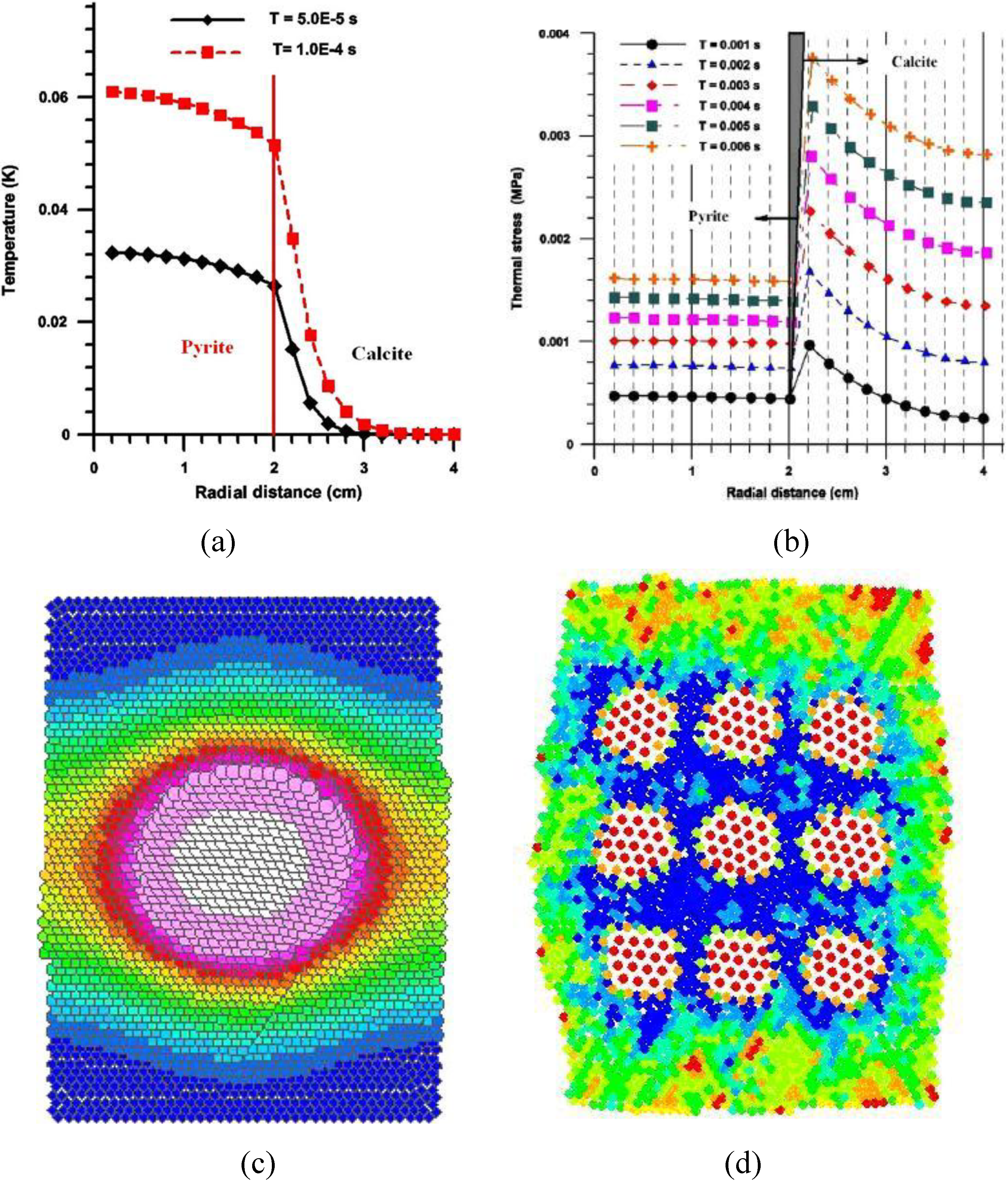
For a polynomial interaction type in Figure 2(c), a piece-wise linearity approximation in Equations (15–17) is adopted.

2.2. Thermal HLPM

Considering thermal effect and material phase change with heating, the following equations are embedded into HLPM [32].
If the time-dependant thermal flow (J/s/m) is given q = κΔT, then, the temperature difference (K) is solved by
Δ T = Δ β m C
where κ is the thermal conductivity tensor (W/m C), m the mass, C the specific heat (J/kg K), and Δβ = Δt · q the change of stored energy (J) per time increment Δt.
Thus, the dynamic change of temperature due to thermal conduction and microwave heating can be determined by
T ( 0 ) = 0.0   K ,    T ( t + Δ t ) = T ( t ) + Δ T + P d / ( C Δ t )
Assuming an isotropic expansion, the final thermally induced strain and stress are given by,
ε t = α ( T t T 0 ) ,   σ t = ε t E ( 1 2 ν )
where ε t is the strain, α is the thermal expansion coefficient (1/K), T t and T 0 is the initial and final temperature, respectively; σ t is the isotropic thermally induced stress. In case of phase change, temperature dependant E versus T should be provided. P d is input power density (W/m3).
Figure 5 exhibits a preliminary HLPM simulation of microwave assisted breakage effect on a calcite-pyrite mixture [32]. In the simulation, the thermally-induced microcracking is found to be along the grain boundaries. This fracture scenario is in a good agreement with the earlier study [33]. Once material phase change information is provided, melting and burning will be simulated. Figure 6 depicts a preliminary HLPM fire resistance study of structure with/without fire proof material coated on the left side. It is seen that without the protection the majority of the structure is burned out, whereas with the protection just a minor amount is burned out.
Figure 5. HLPM simulation of thermally-induced breakage of assemblage of pyrite-calcite, (a), (b) temperature, thermal stress versus radical displacement, (c) spatial temperature distribution within an one inclusion structure, (d) fracture distribution within a nine-inclusion structure. [32].
Polymers 02 00003 g005
Figure 6. HLPM fire resistance study of structure, (a) problem description, (b) with fire proof material coated on the left side, (c) without fire proof material coated on the left side.
Polymers 02 00003 g006
The leapfrog method, with second-order accuracy, is employed in the HLPM simulations. The leapfrog formulas relating position, velocity and acceleration for particles P i ( i = 1 , 2 , ... , N ) [34] are,
V i , 1 / 2 = V i , 0 + ( Δ t ) 2 a   (starter formula)
V i , k + 1 / 2 = V i , k 1 / 2 + ( Δ t ) a i , k k = 1 , 2 , 3 , ...
r i , k + 1 = r i , k + ( Δ t ) V i , k + 1 / 2 k = 0 , 1 , 2 , ...
where V i , k , a i , k and r i , k are the velocity, acceleration and position vectors of particle i at time t k = k Δ t , Δ t is the time step. V i , k + 1 / 2 stands for the velocity of particle i at time t k = ( k + 1 / 2 ) Δ t , and so on. Notably, the leapfrog method is of second-order accuracy: O ( ( Δ t ) 2 ) .
The safe time step is after the derivation result by Hockney & Eastwood [34]:
Ω Δ t < < 2 ,       Ω = ( 1 m | d F d r | max ) 1 / 2

3. Review of HLPM for Polymeric Materials Subject to High Strain Rate Loads

Since its establishment, a number of successful HLPM simulations have been achieved in predicting dynamic fragmentation of polymeric materials (nylon 6-6, vinyl ester and epoxy) with good accuracy compared with the corresponding experimental data. The accomplishments are to be reviewed in the following.

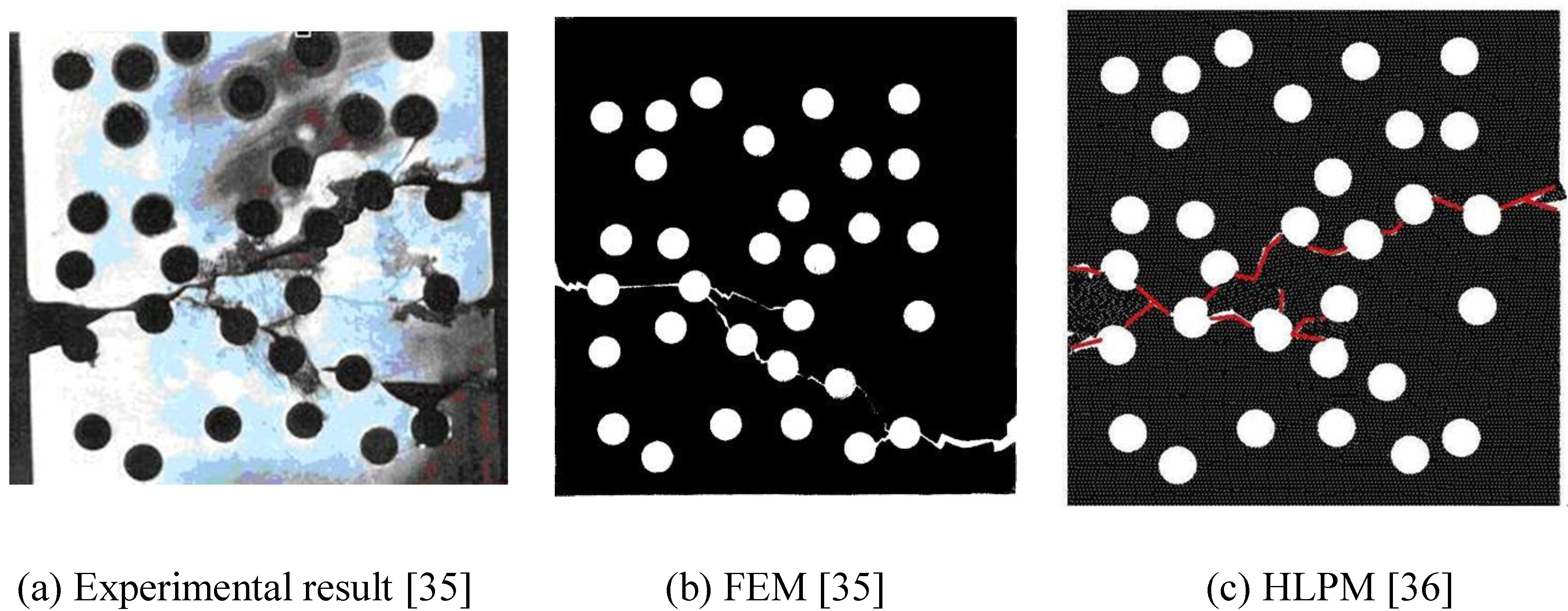
3.1. Prediction of crack pattern in epoxy plate

The first successful application of HLPM has been achieved for simulation of dynamic fragmentation in an (elastic-brittle) epoxy plate (8.25 cm × 33.02 cm), containing non-uniformly distributed circular holes in tension [36]. The average Young modulus of the epoxy is as E ≈ 3.26 GPa, and its tensile strength is σTS = 62.86 MPa, and mass density ρ = 1.1 g/cm3. The elastic–brittle law of particle–particle interactions Equation (15) is employed. Using tensile stress, σTS, from Hooke’s law we can determine the failure strain εmax by
r max r 0 r 0 = ε max = σ T S E
and accordingly the displacement threshold for fracture to occur at rmax.
To readily describe the breakage effect on material, we define a concept of fracture density [32]. By this definition, the local fracture density of particle i, f i d e n . , is equal to the ratio of its current number of broken bonds, N b i to its original number of bonds, N o i , i.e.,
f i d e n . = N b i N o i
It is clearly seen that a big f i d e n . value indicates a severe failure locally occurring at i.
Figure 7(a–c) illustrates the experimental and modelling results of fracture pattern of an epoxy plate with randomly distributed holes in tension. Here is pointed out that, in the simulation, the Poisson's ratio of epoxy was set to 1/3. This is a special case of HLPM in which all the angular interactions are absent [16]. As the figure illustrates, compared with the experimental observation, the HLPM prediction of the crack pattern seems more accurate than that of the FEM solution.
Figure 7. Experimental and modelling results of epoxy in tension, (a) experiment [35], (b) FEM [35], and (c) HLPM simulation [36].
Polymers 02 00003 g007

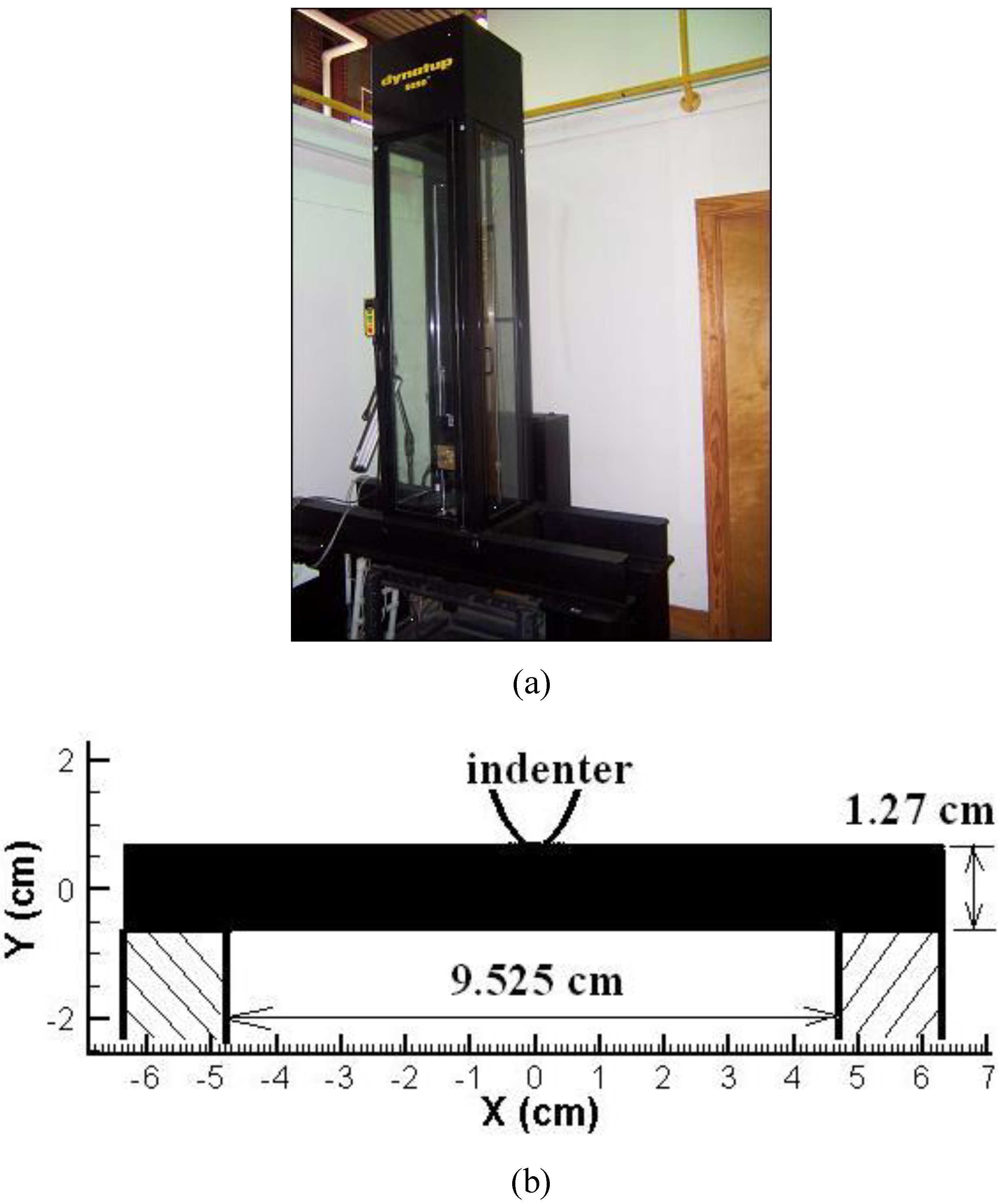
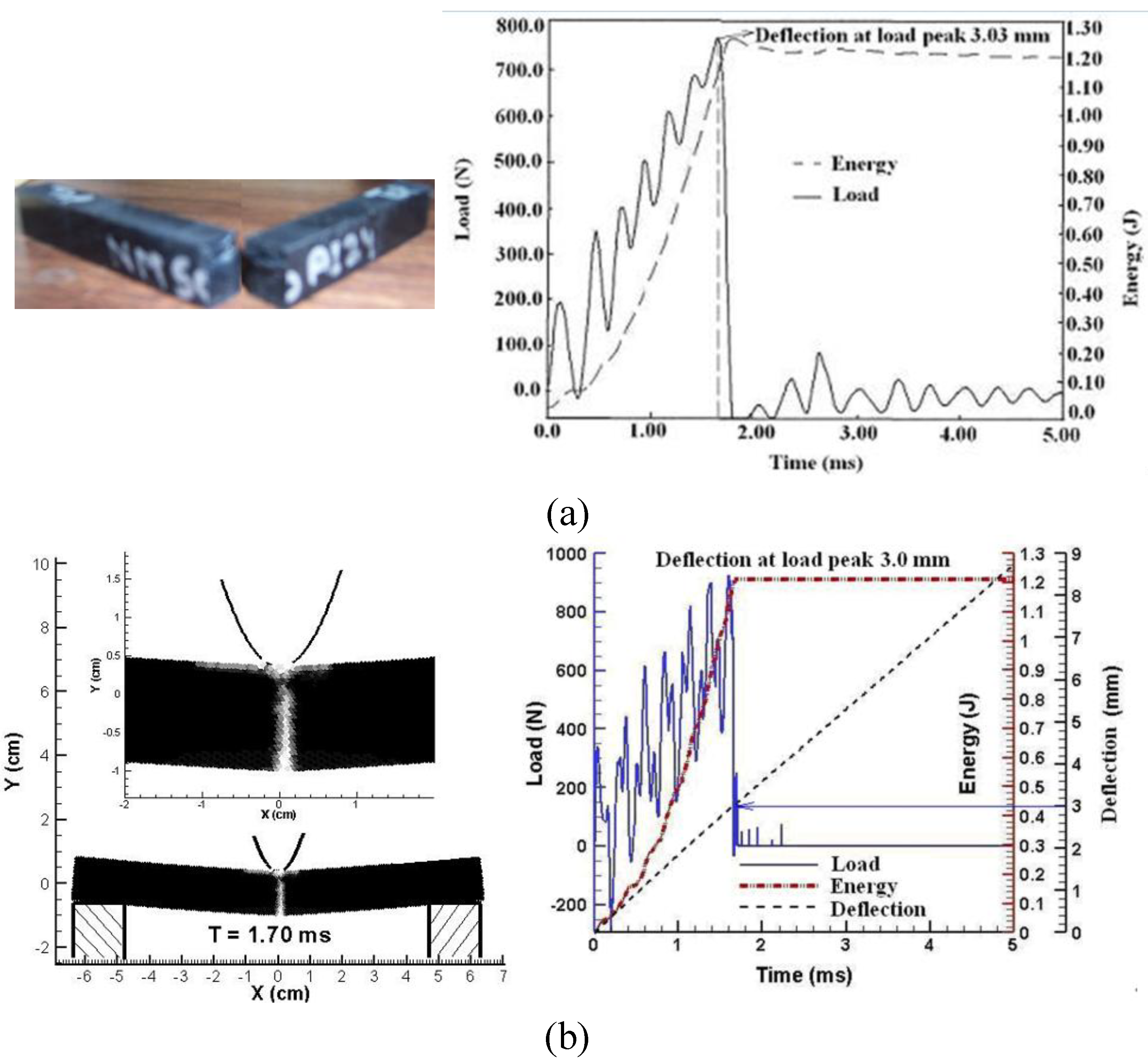
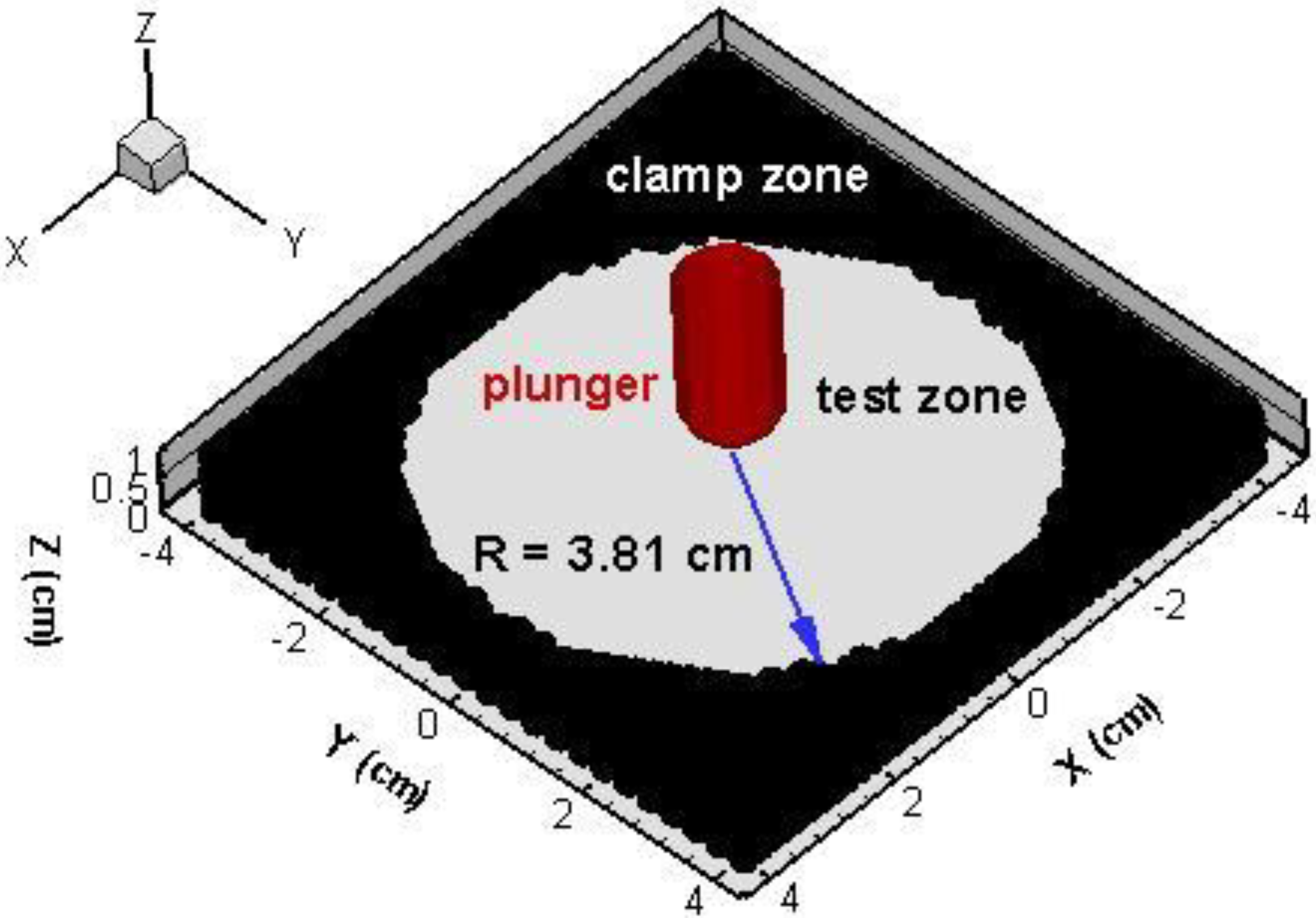
3.2. Indentation of polymeric materials

The nylon-6,6 and vinyl ester impact experiments were conducted in the laboratory of Department of Mechanical Engineering at the University of Mississippi. The sample has the dimensions of (in cm) 12.7 × 12.7 × 0.993 in length, height and width, respectively. The two ends of the sample are simply supported with permission of horizontal movement. Figure 8(a) shows the DYNATUP Model 8250 instrumented impact test machine, and Figure 8(b) illustrates a 2D viewpoint of the specimen setup in the experiment. In an impact process, the indenter is fastened with the drop weight to become an integral impactor. The impactor weighs 3.318 kg. The impactor drops down to the specimen by the action of gravity. After the impactor arrives at the specimen, it is subject to a reaction force from the beam. It is obvious that this whole impact event is a complex, coupled process between the motion of the impactor and the reaction of the polymeric beam. The sensor to measure the resistant load is attached with the impactor.
Figure 8. Impact of indenter to a polymeric material (nylon 6,6 and vinyl ester). (a) Impact test instrument, and (b) dimension of specimen.
Polymers 02 00003 g008
In the impact simulation, the dynamic response of interior particles is easily computed by the corresponding constitutive equations. The challenge comes from how to accurately deal with the exterior particles to be involved into the interaction between the motion of the impactor and the polymeric beam. In the present study, we assume that the indenter is rigid, and the particles interfacing with the indenter surface are pushed away in the direction normal to indenter surface as illustrated in Figure 9. Any tangential movement is neglected. The strategy is implemented as follows.
Figure 9. Implementation of a coupling between rigid impactor and polymeric beam.
Polymers 02 00003 g009
In Figure 9, assuming that at t = t 1 the indenter front, plotted in the dash-dot line, infringes on the particle colored in gray. Let the mass of the impactor be M i m and its instantaneous drop speed be V i m ( t 1 ) . The resistant load from the particle is R F ( t 1 ) . Let the mass of the particle be M p and its instantaneous moving vertical speed be V p ( t 1 ) . After a time increment, at t = t 1 + Δ t , the new drop speed of the indenter can be determined by V i m ( t 1 ) + a i m ( t 1 + Δ t ) × Δ t , where a i m ( t 1 + Δ t ) is the new acceleration value of drop weight that is obtained by M i m a i m ( t 1 + Δ t ) = ( R F ( t 1 ) M i m g ) , and g = 9.80 m/s2 is the gravity acceleration. Consequently, the new indenter profile can be traced along the arrow plotted in Figure 8. Based on this information, the new position of the particle can be calculated, and therefore the displacement is obtained. Taking time derivative of this displacement value, we obtain the new normal velocity of that particle, V p ( t 1 + Δ t ) ; hence, its acceleration, a p ( t 1 + Δ t ) , can be obtained by differentiating the normal velocity with respect to the time increment. Finally, we calculate the resistant force of this particle to the indenter as M p a p ( t 1 + Δ t ) . Summing all force on the interfacing particles enables us to obtain the total resistant force to the indenter. After the computation is finished for the present time step, these results become the initial conditions for the next time step. This process continues until the computation ends.
HLPM of nylon-6,6 and vinyl ester indentation study are to be shown in the following.

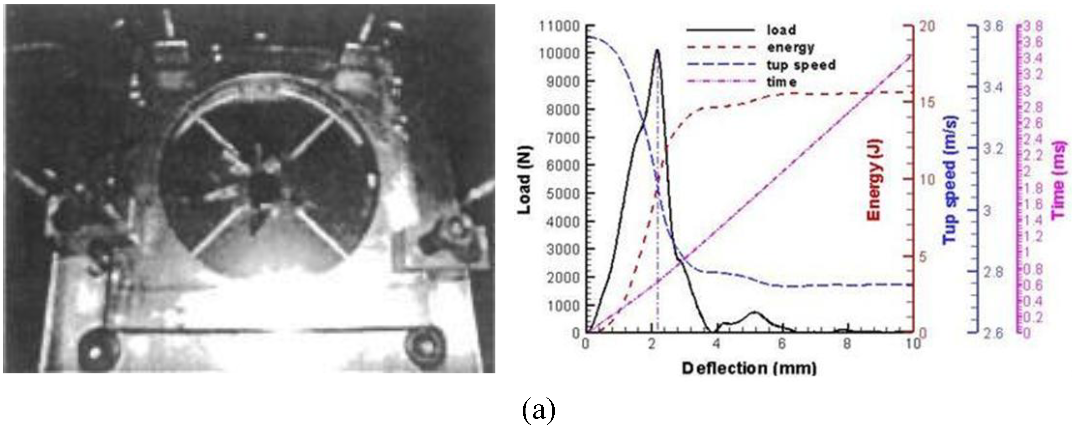
3.2.1. Indentation of nylon-6,6

The measured maximum impact velocity of the impactor arriving at the surface of the beam is 1.87 m/s. The density of the material is 1,140 kg/m3. The Young’s modulus and the tensile strength are E = 3.0 GPa and σTS = 60 MPa, respectively.
The similar linearity constitutive equations as used in Section 3.1 are applied. However, to predict fracture patterns more accurately, a two-layer particle interaction scheme (nearest-second neighboring particle interaction, Figure 3(b)) is adopted. The effective bond stiffness with this new interaction network is derived following the equivalence of the associated material’s physical property, i.e., Young’s modulus [16].
Figure 10a,b depicts the comparison of experimental and HLPM results [30]. It is found that (1) PM modelling crack pattern agrees with the associated observation, and (2) it is seen that measured load peak happens around t ≈ 1.70 ms, and the measured deflection at the load peak is 3.03 mm, with the total impact energy equal to 1.2 J. The corresponding HLPM simulated result shows that the load peak happens around t ≈ 1.66 ms, and the deflection at load peak is 3.0 mm, and the total impact energy calculated is 1.2 J. Although the simulated load profile is not exactly the same as the experiment, we observe similar characteristics, including the fluctuating profile with roughly the same period. The simulated peak load is also reasonable close to the experimental value. Hence we conclude that the HLPM simulation compares favorably with the experimental measurements.
Figure 10. The study of the failure of nylon-6, 6 due to the impact of a rigid indenter (a) experimental results; (b) HLPM results. Maximum drop velocity of indenter is 1.87 m/s [30].
Polymers 02 00003 g010

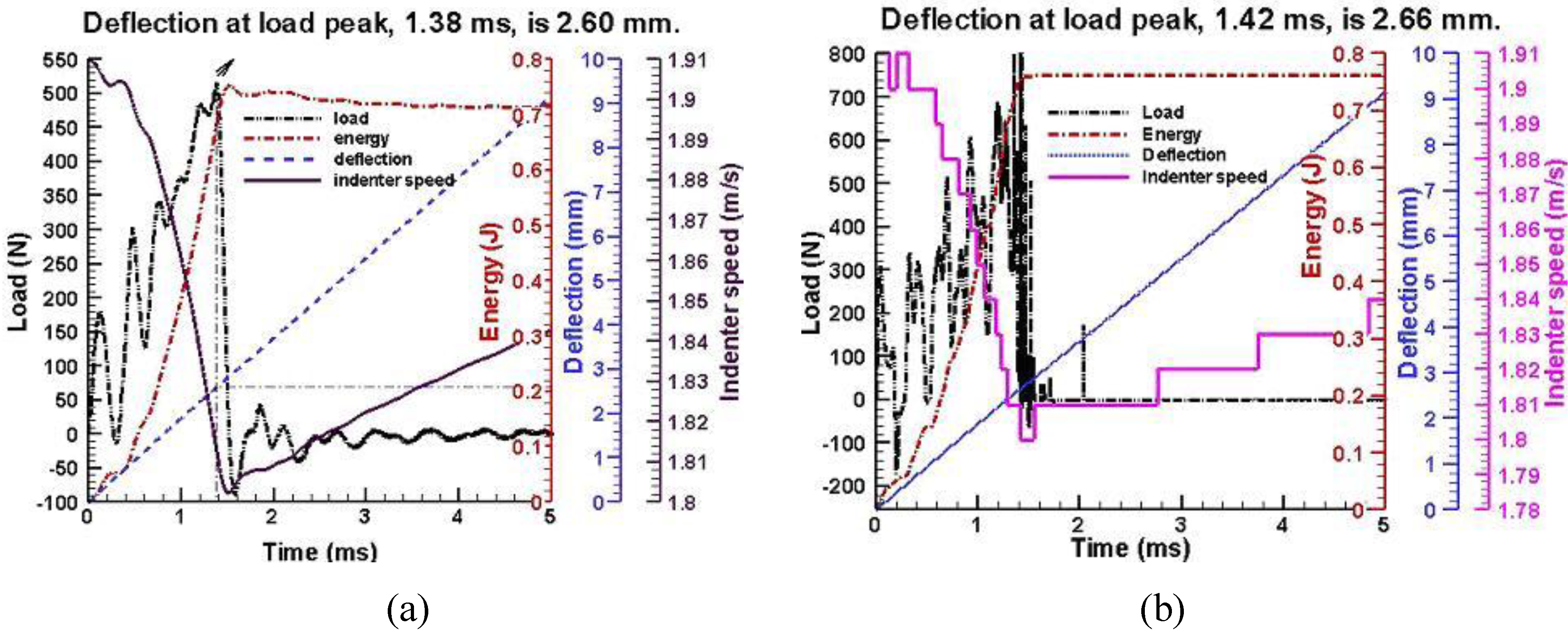
3.2.2. Indentation of vinyl ester

The measured maximum impact velocity of the impactor arriving at the surface of the beam is 1.91 m/s. The density of the material is 1,050 kg/m3. The Young’s modulus and the tensile strength are E ≈ 2.56 GPa, and σTS = 25.6~51.2 MPa, respectively.
A exactly the same modelling method as used in Section 3.2.1 is employed in the following. Figure 11a,b depicts the comparison of experimental and HLPM results [37]. It is seen that measured load peak happens around t ≈ 1.38 ms, and the measured deflection at the load peak is 2.60 mm, with the total impact energy equal to 0.7 J. The corresponding HLPM simulated result shows that the load peak happens around t ≈ 1.42 ms, and the deflection at load peak is 2.66 mm, and the total impact energy calculated is 0.76 J. Similarly to Figure 10a,b, although the simulated load profile is not exactly the same as the experiment, we observe similar characteristics, including the fluctuating profile with roughly the same period. The simulated peak load is also reasonable close to the experimental value. Hence we conclude again that the HLPM simulation compares favorably with the experimental measurements.
Figure 11. Comparison of HLPM result with the according experimental observation of the failure of vinyl ester due to the impact of a rigid indenter, (a) experimental observation, (b) HLPM simulation. Maximum drop velocity of indenter is 1.91 m/s [37].
Polymers 02 00003 g011

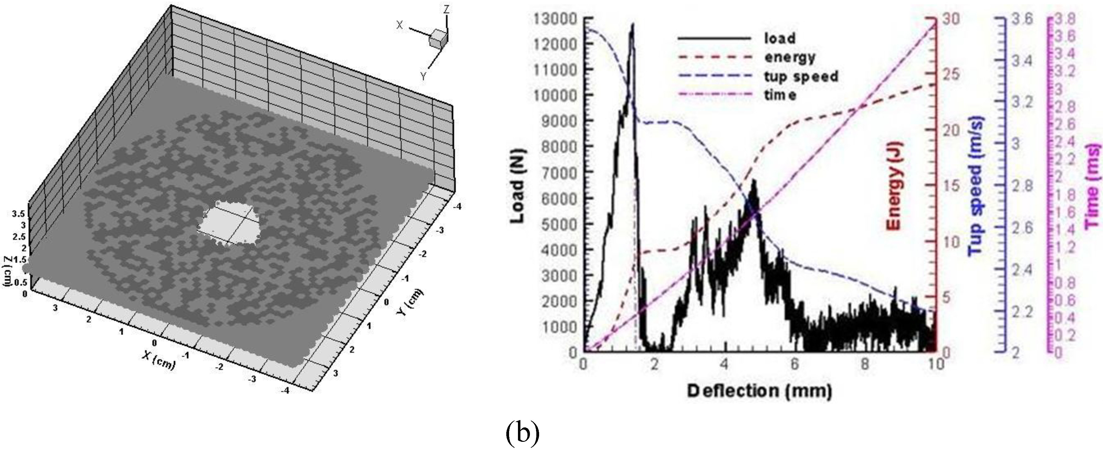
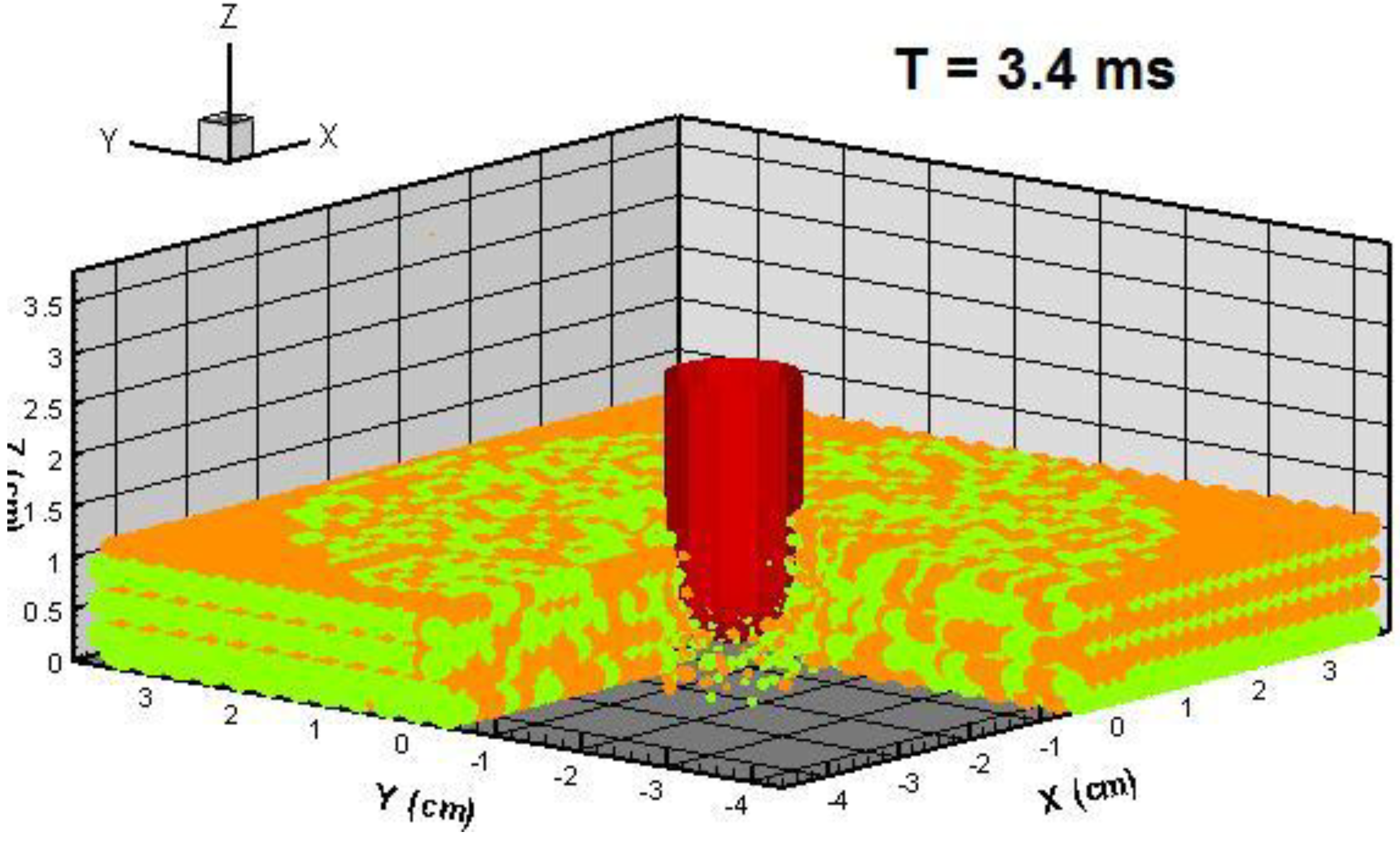
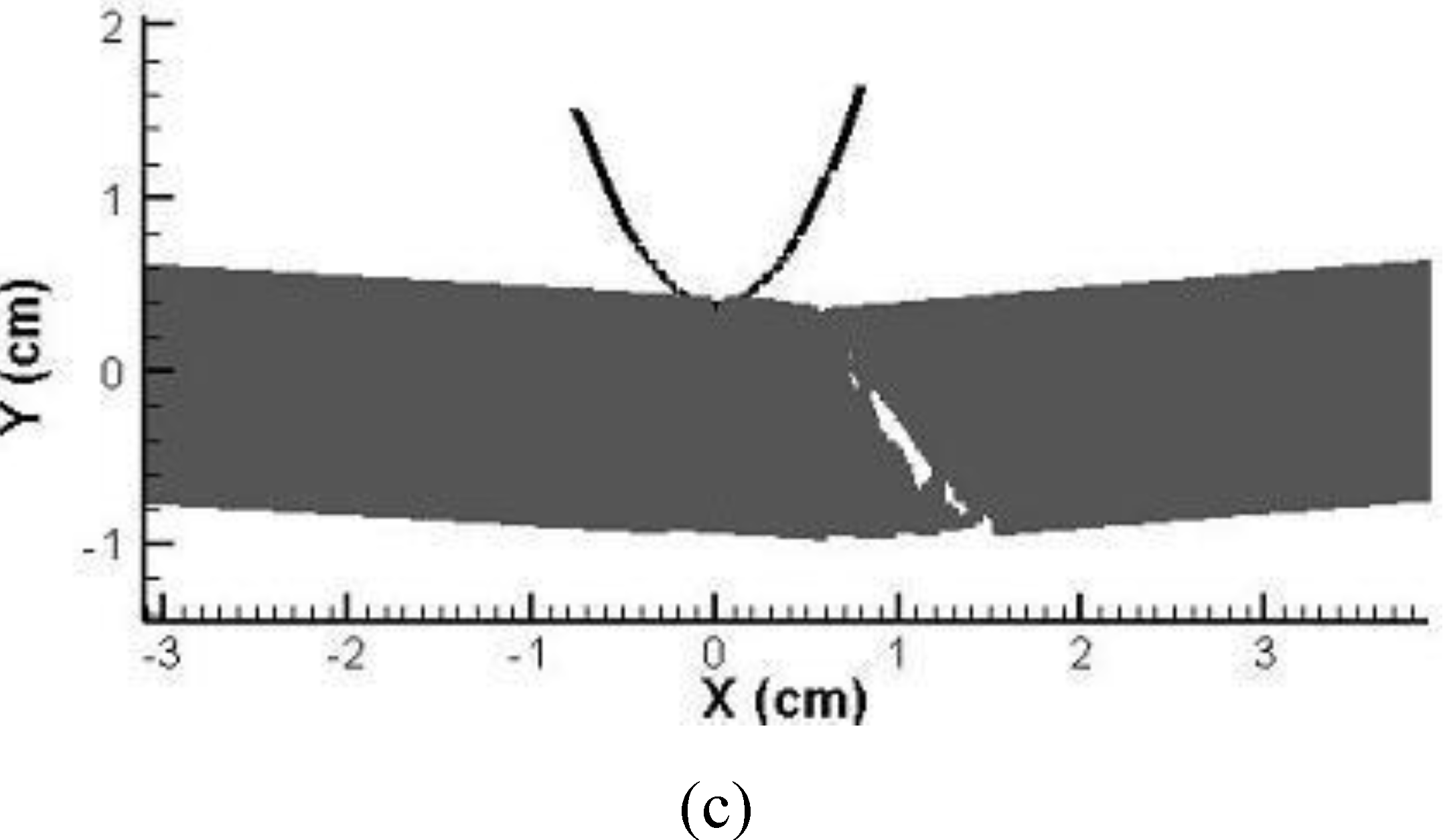
3.2.3. Punctuation of vinyl ester

The impactor weighs 5.95 kg, and the measured maximum impact velocity of the impactor reaching the surface of the plate is 3.55 m/s. The sample has the dimensions of (in cm) 10.16 × 10.16 × 1.0 in length, width and thickness, respectively. Each specimen's top and bottom surfaces were clamped only with a 3.81 cm hole in radius at the center, see Figure 12. Such setting is to center the specimen for uniform gripping and enough tighten the clamping so as to provide uniform clamping pressure to prevent slippage during the tests.
Figure 12. Setup of specimen for punch-shear test of vinyl ester plate.
Polymers 02 00003 g012
A 3D HLPM has been built up. The 3D particle-particle interaction approximately employs the 2D derivation result. Figure 13a,b compares the experimental with the HLPM result. It is seen that the observed puncture area and shape on the specimen is similar to that of the HLPM prediction. Although the simulated load profile has a visual difference from the experiment, we observe similar characteristics, including the fluctuating profile with roughly the same tendency. Especially, the comparison is satisfactory at the damage initiation stage—from the moment of impact to the point of peak load, with the measured load peak equal to 10,000.0 N occurring around a deflection of 2.1 mm while the two according HLPM results are 12,800.0 N vs. 1.6 mm. However, the HLPM underpredicts the duration of puncture propagation stage—from the point of peak load (puncture initiation) to the zero load point (puncture completion), and overpredicts the duration and magnitude of post puncture shear stage—dominated by the shear effect of the available puncture peripheral surface of the specimen and the plunger surface.
Figure 13. The study of 3D punch-shear of vinyl ester (a) experimental results; (b) HLPM results. Maximum drop velocity of indenter is 3.55 m/s.
Polymers 02 00003 g013aPolymers 02 00003 g013b
The above-mentioned discrepancies may be due to two major factors. First, the 3D HLPM simulation shown here still employs the same contact method as in [30,37], in which a rigid plunger is assumed, and the particles interfacing with the plunger surface are assumed to be pushed away in the direction normal to plunger surface. This is a completely non-slip contact assumption. To improve the accuracy of HLPM at the damage initiation stage, a partial-slip contact mode may help. For the puncture propagation stage and the post puncture shear stage, where the hinging effects of attached fragments with the surface of the plunger, the shear effect of the available puncture peripheral surface of the specimen and the plunger surface are dominant, our post-fractured particle-to-particle interaction scheme needs to be improved.
Nevertheless, we can conclude that the 3D HLPM can well predict the punch-shear process of a vinyl ester platelet, especially during the damage initiation stage.
Figure 14 shows a snapshot of HLPM prediction of plunger puncture into the sample. It provides a clear insight into the interaction of the plunger with the material and the resultant fracture inside.
Figure 14. Snapshot of HLPM prediction of fracture of punch-shear of vinyl ester at T = 3.4 ms. Maximum drop velocity of indenter is 3.55 m/s.
Polymers 02 00003 g014

4. HLPM Prediction of Wave Propagation and Wave Induced Fracture

4.1. HLPM prediction of wave propagation in 1D and 2D elastic-brittle material

In this section we first review our HLPM study of wave propagation in a 1D and 2D elastic-brittle bar, subjected to dynamic and kinematic loads, respectively, [38]. The computational domain for 1D and 2D are L = 12.7 cm in length (one layer of particles) and 12.7 cm × 12.7 cm (fifteen layers of particles), respectively, with an initial particle spacing r0 = 0.1 cm; two points are selected at L/4 and L/2 away from the left end for calculating the wave propagation speed. Dynamic and kinematic conditions are, respectively, applied to the left end at 97.8 MPa and constantly 60.0 m/s; the right end is fixed and the remaining boundaries are traction free. The material parameters are: Young's modulus E = 3.0 GPa, density ρ = 1,140 kg/m3, and failure strain εmax = 0.02. For simplicity, we assume that the Poisson's ratio of the material is equal to 1/3. Consequently, the angular spring effect is absent [16], and only the axial interaction is accounted for and determined after Equation (15).
The classical wave theory gives that the wave propagation speeds in the above-mentioned 1D and 2D material bars are, respectively [39],
1 D :   C p ( 1 D ) = E / ρ 1622.0   m / s
2 D :   C p ( 2 D ) = ( K + 4 G / 3 ) / ρ 1986.0   m / s
with K and G the bulk and shear modulus, respectively.

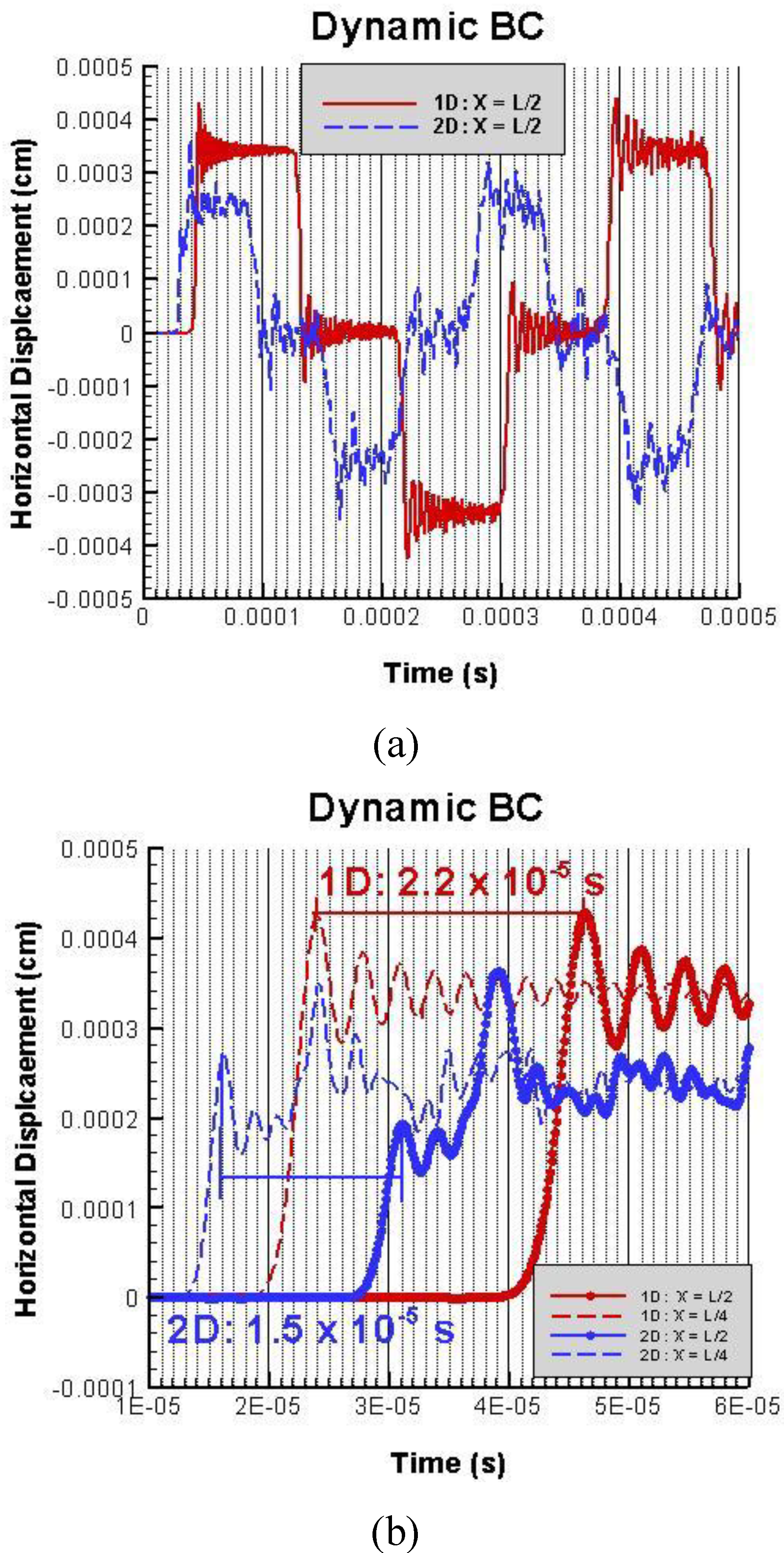
4.1.1. Dynamic boundary condition

A dynamic boundary condition with 97.8 MPa is applied to the left end of 1D and 2D bar, respectively. Figure 15 displays the HLPM results of the horizontal displacement for 1D and 2D at X = L/2. From Figure 15(a) it is seen that the wave propagation profiles of 1D and 2D are different from each other due to the existing difference of wave propagation speed in 1D from in 2D structure. Via Figure 15(b), we can calculate that the horizontal wave speed values travelling in the 1D and 2D bar are equal to 1,455.0 m/s and 2,133.0 m/s, respectively. These results indicate that, the 1D simulation result is smaller than the analytical solution, 1,622.0 m/s, while the 2D result is bigger than the analytical value, 1,986.0 m/s. The reason for the existing discrepancies is not very clear. It may arise from the difference of wave propagation in lattice-particle structure from that of the continuum media. However, we can still conclude that HLPM is able to correctly capture the wave propagation of solids.
Figure 15. HPLM prediction of horizontal displacement for 1D and 2D bar, respectively. (a) horizontal displacement recorded at X = L/2; (b) horizontal displacement recorded at X = L/4 and X = L/2. Dynamic boundary condition is applied, [38].
Polymers 02 00003 g015

4.1.2. Kinematic boundary condition

A kinematic boundary condition with 60.0 cm/s is constantly applied to the left end of the 1D and 2D bar, respectively. Figure 16 displays the HLPM results of the horizontal displacement for the 1D and 2D simulations at X = L/2. From Figure 16(a) it is seen that the wave propagation profiles for both of the 1D and 2D cases are equally increased in amplitude after each period of wave reflection; this coincides with the knowledge of wave propagation with a constant load condition. Via Figure 16(b), we can calculate that the horizontal wave speed value for 1D and 2D cases are equal to 1,455.0 m/s and 2,133.0 m/s, respectively. These values are similar to the above-shown 1D and 2D cases subject to a dynamic load.
Figure 16. HPLM prediction of horizontal displacement for 1D and 2D bar, respectively. (a) horizontal displacement recorded at X = L/2; (b) horizontal displacement recorded at X = L/4 and X = L/2. Kinematic boundary condition is applied [38].
Polymers 02 00003 g016

4.2. HLPM study of wave induced fracture—spall crack formation

In this section we review our HLPM study of wave induced fracturespall crack formation. Spall crack formation is the direct consequence arising from the wave (tensile and compressive wave) interactions in solids. The area will be highly stretched wherever the strong enough tensile and compressive waves meet, and a spall crack will consequently occur.
The dimension of the target is set as 5.2 cm × 0.68 cm while the two different sizes of the flyer are set as 5.2 cm × 0.20 cm and 2.6 cm × 0.20 cm, respectively. The material properties of flyer and target are set to be identical, in which the Young's modulus is E = 163.24 GPa, the tensile strength σTS = 478.25 MPa, failure strain εmax = 0.10, and density ρ = 8,900.0 kg/m3. The flyer's initial dropping speed is 260.0 m/s. Traction free boundary conditions are applied to all the boundaries.
Figure 17 shows the qualitative comparison of spall crack formation of HPLM simulations with the results obtained from the analogous molecular dynamic (MD) simulations by Krivtsov [40,41]. As seen from Figure 17(b), the spall crack formation is clearly captured by HLPM. We see that the tensile wave—the wave reflected from the bottom of the target, meets the compressive wave—the wave reflected from the top of the flyer, at a thin layered area with a distance away from the bottom of the target. The two types of wave propagate in different directions alongside the Y-axis when they meet; this leads to a high stretching to the material herein, thus a spall crack zone is generated. It is also observed that the predicted length of spall crack formation is smaller than that of the flyer and the height of the lower spalling part is the same as that of the flyer. This matches with the MD results [40,41].
Figure 17. Qualitative comparison of spall crack formation of HPLM with MD. (a) MD simulations, [40,41] (b) HLPM simulations. Impact speed = 260.0 m/s, [38].
Polymers 02 00003 g017

5. Concluding Remarks

In this paper, we review a number of accomplishments of HLPM in the dynamic fragmentation of polymeric materials with good accuracy. Nylon 6-6, vinyl ester and epoxy are accounted for under the loading conditions of tension, indentation and punctuation. In addition, HLPM of wave propagation and wave induced fracture study is also reviewed.
From the demonstrations of the obtained HLPM simulation results, we can summarize several important conclusions:
(1)
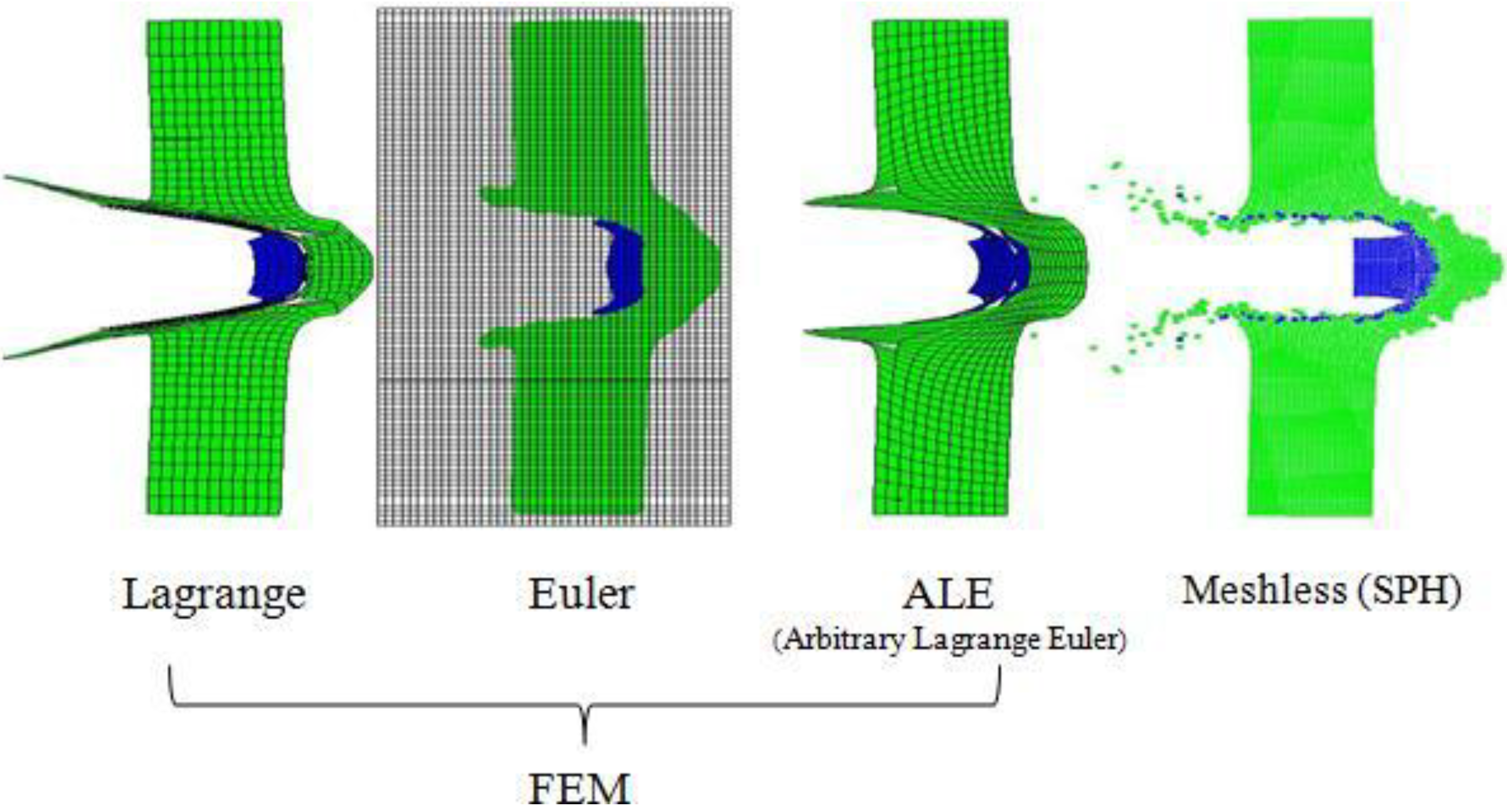
No need for remeshing. Re-meshing is known as an overwhelming challenge for FEM whereas HLPM does not suffer from it at all. In HLPM, fracture is created when a bond (spring) is broken by translational force. This provides HLPM a unique power to be able to quite easily overcome the “discontinuity of material” problem.
(2)
No stress intensity required. In HLPM, a bond (spring) is broken and fracture is thus resulted wherever the critical failure strain is reached.
(3)
HLPM can accurately predict the dynamic fragmentation of polymeric materials under high strain rate loading conditions, and can correctly capture wave propagation of solids.
In conclusion, our HLPM model provides a powerful simulation tool. However, more work is needed to verify it further, and future work should focus on:
(1)
Genuine 3D interaction force formulas that will be developed following Keating's approach [31].
(2)
More adequate impact mode will be developed so as to accurately describe the shear friction between the projectile and the penetrated target.
(3)
Rigorous validation work will continuously validate and calibrate the HLPM model, and test its suitability to different physical problems.
(4)
HLPM will be employed in various important applications, such as impact, blasting, thermally-induced breakage problems.

Acknowledgement

The authors wish to acknowledge the anonymous reviewer's valuable comments.

References

  1. Ferry, J.D. Viscoelastic Properties of Polymers, 3rd ed.; John Wiley & Sons: Hoboken, NJ, USA, 1980; Chapter 11. [Google Scholar]
  2. Mishra, S.; Sonawane, S.; Chitodkar, V. Comparative Study on Improvement in Mechanical and Flame Retarding Properties of Epoxy-CaCO3 Nano and Commercial Composites. Polym. Plast. Technol. Eng. 2005, 44, 463–473. [Google Scholar] [CrossRef]
  3. Wang, Z.; Massam, J.; Pinnavaia, T.J. Epoxy-Clay Nano Composites. In Polymer-Clay Nano Composites; Wiley: Hoboken, NJ, USA, 2000; pp. 127–148. [Google Scholar]
  4. Zhu, J.; Imam, A.; Crane, R.; Lozano, K.; Khabashesku, V.N.; Barrera, E.V. Processing a Glass Fiber Reinforced Vinyl Ester Composite with Nanotube Enhancement of Interlaminar Shear Strength. Compos. Sci. Technol. 2007, 67, 1509–1517. [Google Scholar] [CrossRef]
  5. Xia, Z.; Ellyin, F. Time-Dependent Behaviour and Viscoelastic Constitutive Modelling of an Epoxy Polymer. Polym. Polym. Compos. 1998, 6(No. 2). [Google Scholar]
  6. ASTM Standard D-4065-01; Standard Practice for Plastics: Dynamic Mechanical Properties: Determination and Report of Procedures; ASTM International: West Conshohocken, PA, USA, 2000.
  7. Hutton, D.V. Fundamentals of Finite Element Analysis; McGraw-Hill: New York, NY, USA, 2004. [Google Scholar]
  8. Quan, X.; Birnbaum, N.K.; Cowler, M.S.; Gerber, B.I.; Clegg, R.A.; Hayhurst, C.J. Numerical Simulation of Structural Deformation under Shock and Impact Loads Using a Coupled Multi-Solver Approach. In Proceedings of the 5th Asia-Pacific Conference on Shock and Impact Loads on Structures, Hunan, China, November 12–14, 2003.
  9. Belytschko, T.; Loehnert, S.; Song, J.H. Multiscale Aggregating Discontinuities: A Method for Circumventing Loss of Material Stability. Int. J. Numer. Meth. Engng. 2008, 73, 869–894. [Google Scholar] [CrossRef]
  10. Monaghan, J. Smoothed Particle Hydrodynamics. Rep. Prog. Phys. 2005, 68, 1703–1759. [Google Scholar] [CrossRef]
  11. Cundall, P.A. Computer Simulations of Dense Sphere Assemblies. In Micromechanics of Granular Materials; Satake, M., Jenkins, J.T., Eds.; Elsevier: Amsterdam, The Netherlands, 1988; pp. 113–123. [Google Scholar]
  12. Meguro, M.; Tagel-Din, H. Applied Element Method for Structural Analysis: Theory and Application for Linear Materials. Structural Eng./Earthquake Eng., JSCE 2000, 17, 1–14. [Google Scholar]
  13. Wang, G.; Ostoja-Starzewski, M.; Radziszewski, P.; Ourriban, M. Particle Modelling of Dynamic Fragmentation-II: Fracture in Single- and Multi-Phase Materials. Comp. Mat. Sci. 2006, 35, 116–133. [Google Scholar] [CrossRef]
  14. Wang, G.; Ostoja-Starzewski, M. Particle Modelling of Dynamic Fragmentation-I: Theoretical Considerations. Comput. Mater. Sci. 2005, 33, 429–442. [Google Scholar] [CrossRef]
  15. Wang, G.; Al-Ostaz, A.; Cheng, A.H.D.; Radziszewski, P. Particle Modelling and Its Current Success in the Simulations of Dynamic Fragmentation of Solids. In Strength of Materials; Nova Science Publishers: New York, NY, USA, 2009; pp. 157–182. [Google Scholar]
  16. Wang, G.; Al-Ostaz, A.; Cheng, A.H.D.; Mantena, P.R. Hybrid Lattice Particle Modelling: Theoretical Considerations for a 2-D Elastic Spring Network for Dynamic Fracture Simulations. Comput. Mater. Sci. 2009, 44, 1126–1134. [Google Scholar] [CrossRef]
  17. Oñate, E.; Idelsohn, S.R.; Pin, F.D.; Aubry, R. The Particle Finite Element Method. An Overview. Int. J. Comput. Method 2004, 1, 267–307. [Google Scholar] [CrossRef]
  18. Chen, Z.; Brannon, R. An Evaluation of the Material Point Method; Sand Report; Sandia National Laboratories: Livermore, CA, USA, 2002.
  19. Cusatis, G.; Zdenek, Z.P.; Cedolin, L. Confinement-Shear Lattice Model for Concrete Damage in Tension and Compression: I. Theory. ASCE J. Engrg. Mech. 2003, 129, 1439–1448. [Google Scholar] [CrossRef]
  20. Cusatis, G.; Zdenek, Z.P.; Cedolin, L. Confinement-Shear Lattice Model for Concrete Damage in Tension and Compression: II. Computation and Validation. ASCE J. Engrg. Mech. 2003, 129, 1449–1458. [Google Scholar] [CrossRef]
  21. Belytschko, T.; Organ, D.; Gerlach, C. Element-Free Galerkin Methods for Dynamic Fracture in Concrete. Comp. Methods Appl. Mech. Engrg. 2000, 187, 385–399. [Google Scholar] [CrossRef]
  22. Liu, W.K.; Jun, S.; Zhang, Y.F. Reproducing Kernel Particle Methods. Int. J. Numer. Methods Fluids 2005, 20, 1081–1106. [Google Scholar] [CrossRef]
  23. Melenk, J.M.; Babuska, I. The Partition of Unity Finite Element Method: Basic Theory and Applications. Comp. Methods Appl. Mech. Engrg. 1996, 139, 289–314. [Google Scholar] [CrossRef]
  24. Babuska, I.; Melenk, J.M. The Partition of Unity Method. Int. J. Numer. Methods Engrg. 1997, 40, 727–758. [Google Scholar] [CrossRef]
  25. Belytschko, T.; Krongauz, Y.; Organ, D. Meshlessmethod: An Overview and Recent Development. Comp. Methods Appl. Mech. Engrg. 1996, 139, 3–47. [Google Scholar] [CrossRef]
  26. Ostoja-Starzewski, M. Lattice Models in Micromechanics. Appl. Mech. Rev. 2002, 55, 35–60. [Google Scholar] [CrossRef]
  27. Fred, I. Numerical Simulation of Differential Equations; Academic Press: New York, NY, USA, 1979. [Google Scholar]
  28. Zukas, J. Introduction to Hydrocodes; Elsevier: Amsterdam, The Netherlands, 2004. [Google Scholar]
  29. Ashby, M.F.; Jones, D.R.H. Engineering Materials 1: An Introduction to Their Properties and Applications; Pergamon Press: New York, NY, USA, 1980. [Google Scholar]
  30. Wang, G.; Al-Ostaz, A.; Cheng, A.H.D.; Mantena, P.R. Particle Modelling of a Polymeric Material (Nylon-6, 6) due to the Impact of a Rigid Indenter. Comp. Mat. Sci. 2008, 44, 449–463. [Google Scholar] [CrossRef]
  31. Keating, P.N. Relationship between the Macroscopic and Microscopic Theory of Crystal Elasticity. I. Primitive Crystals. Phys. Rev. 1966, 152, 774–779. [Google Scholar] [CrossRef]
  32. Wang, G.; Radziszewski, P.; Ouellet, J. Particle Modelling Simulation of Thermal Effects on Ore Breakage. Comp. Mat. Sci. 2008, 43, 892–901. [Google Scholar] [CrossRef]
  33. Walkiwicz, J.W.; Kazonich, G.; McGill, S.L. Microwave heating characteristics of selected minerals and compounds. Miner. Metallurg. Process. 1988, 5, 39–42. [Google Scholar]
  34. Hockney, R.W.; Eastwood, J.W. Computer Simulation Using Particles; Institute of Physics Publishing: Philadelphia, PA, USA, 1988. [Google Scholar]
  35. Al-Ostaz, A.; Jasiuk, I. Crack Initiation and Propagation in Materials with Randomly Distributed Holes. Eng. Fract. Mech. 1997, 58, 395–420. [Google Scholar] [CrossRef]
  36. Ostoja-Starzewski, M.; Wang, G. Particle Modelling of Random Crack Patterns in Epoxy Plates. Probab. Eng. Mech. 2006, 21, 267–275. [Google Scholar] [CrossRef]
  37. Wang, G. Particle Modelling of Polymeric Material Indentation Study. Eng. Fract. Mech. 2009, 76, 1386–1395. [Google Scholar]
  38. Wang, G.; Al-Ostaz, A.; Cheng, A.H.D.; Mantena, P.R. Hybrid Lattice Particle Modelling of Wave Propagation Induced Fracture of Solids. Comp. Methods Appl. Mech. Eng. 2009, 199, 197–205. [Google Scholar] [CrossRef]
  39. Meyers, M.A. Dynamic Behavior of Materials; Wiley-interscience: Malden, MA, USA, 1994. [Google Scholar]
  40. Krivtsov, A.M. Relation between Spall Strength and Mesoparticle Velocity Dispersion. Int. J. Impact Eng. 1999, 23, 477–487. [Google Scholar] [CrossRef]
  41. Krivtsov, A.M. Computer Simulation of Spall Crack Formation. In Proceedings of the 4th European Conference on Structural Dynamics, Eurodyn'99, Prague, Czech Republic, June 7–10, 1999; pp. 475–477.

