Machine Learning Approaches for the Prioritization of Genomic Variants Impacting Pre-mRNA Splicing


Abstract
1. Introduction
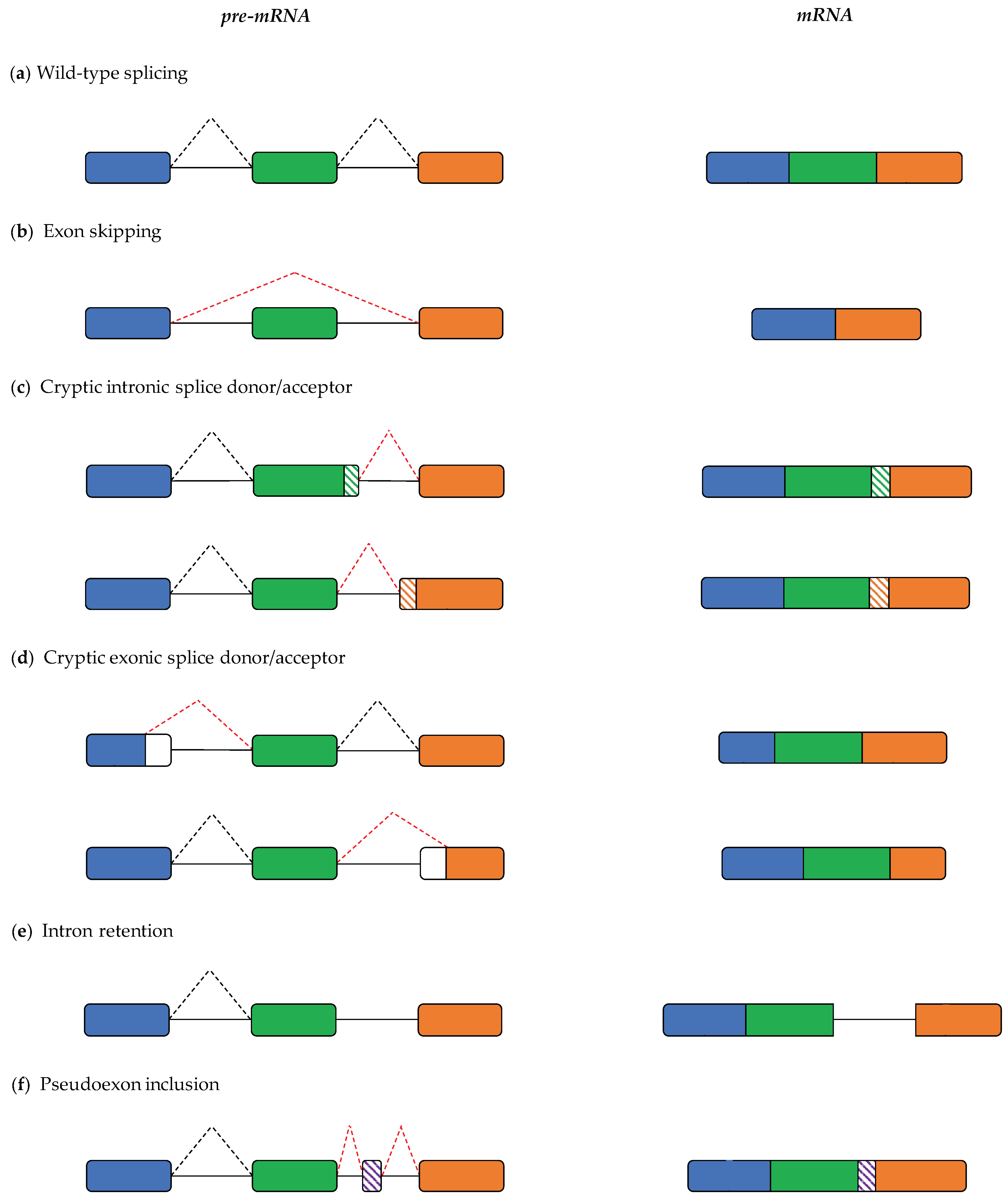
2. Pre-mRNA Splicing and Its Role in Pathogenesis
3. Early Computational Methodologies to Prioritize Genomic Variants Impacting Splicing
4. Basics of Machine Learning Techniques
4.1. Basics of Machine Learning
4.2. Features
4.3. Training and Test Sets
4.4. Outputs
4.5. Model Evaluation
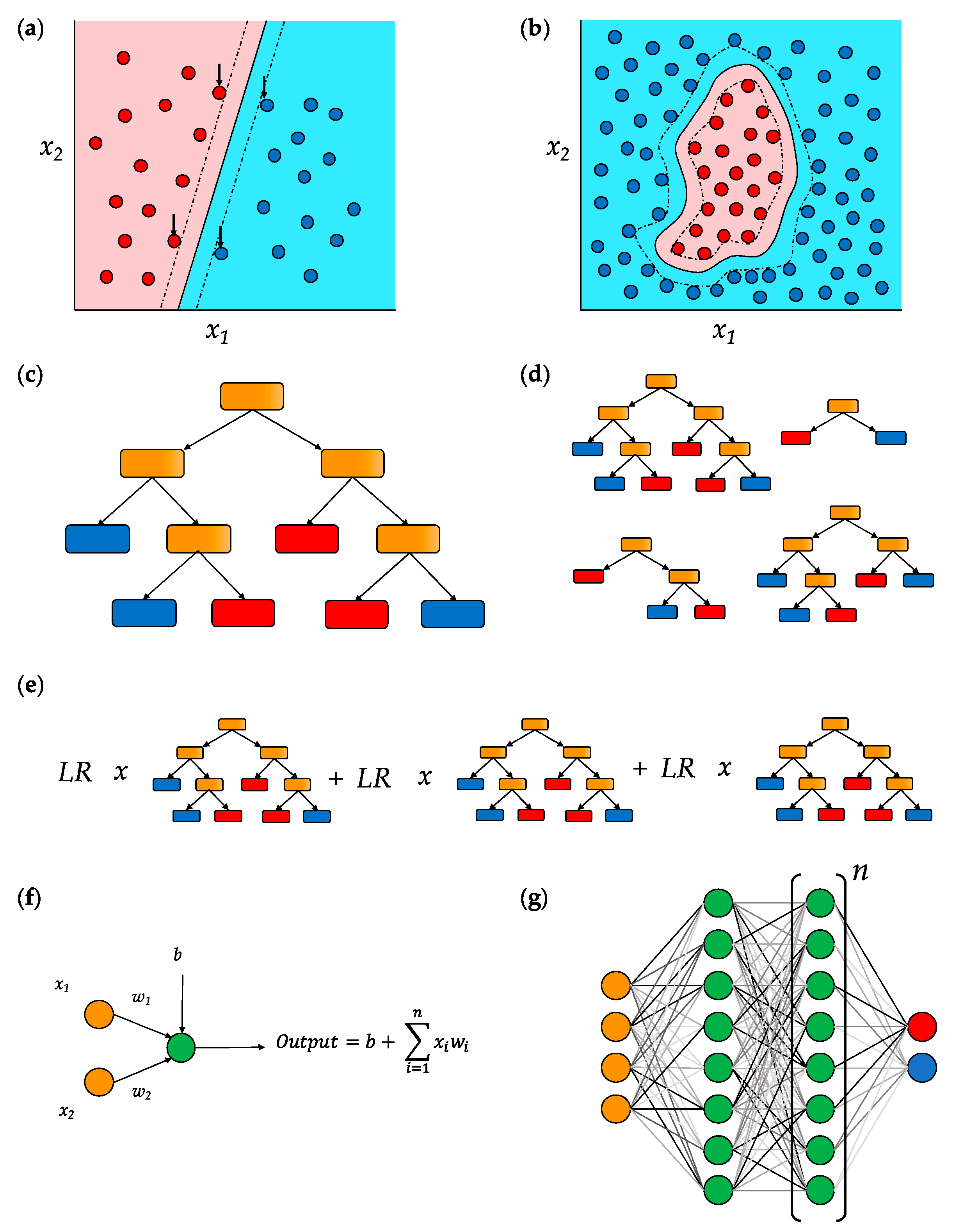
5. Common Machine Learning Models in Splice Prediction
5.1. Support Vector Machines (SVMs)
5.2. Decision Trees
5.3. Deep Neural Networks (DNNs)
6. Machine Learning-Based Tools for Splicing Prediction
6.1. CADD (Combined Annotation-Dependent Depletion)
6.2. TraP (Transcript-Inferred Pathogenicity) Scores
6.3. SPANR (Splicing-Based Analysis of Variants)
6.4. CryptSplice
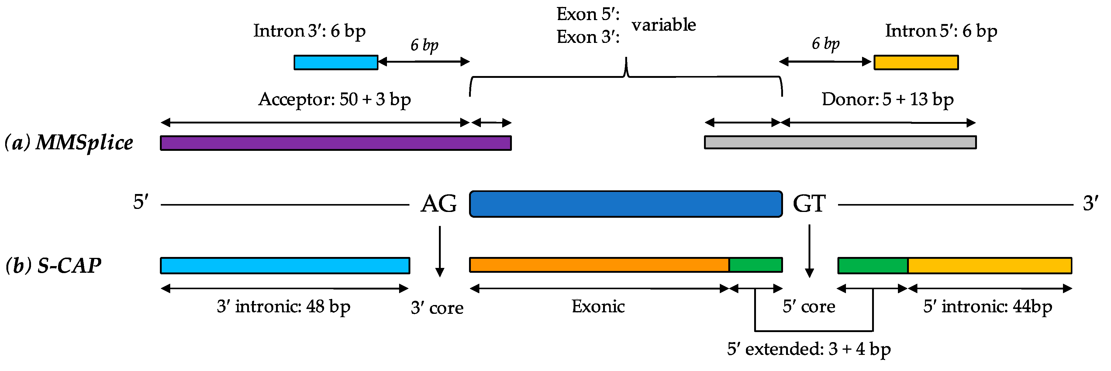
6.5. MMSplice (Modular Modeling of Splicing)
6.6. S-CAP (Splicing Clinically Applicable Pathogenicity Prediction)
6.7. SpliceAI
7. Discussion
Supplementary Materials
Funding
Conflicts of Interest
References
- Zayed Centre for Research into Rare Disease in Children. Scale of Rare Diseases. Available online: https://www.gosh.org/what-we-do/research/zayed-centre-research-rare-disease-children/rare-diseases/scale-rare-diseases (accessed on 14 October 2019).
- National Health Service (NHS) England. National Genomic Test Directory. Available online: https://www.england.nhs.uk/publication/national-genomic-test-directories/ (accessed on 26 October 2019).
- Ellingford, J.M.; Barton, S.; Bhaskar, S.; O’Sullivan, J.; Williams, S.G.; Lamb, J.A.; Panda, B.; Sergouniotis, P.I.; Gillespie, R.L.; Daiger, S.P.; et al. Molecular findings from 537 individuals with inherited retinal disease. J. Med. Genet. 2016, 53, 761–767. [Google Scholar] [CrossRef]
- Henn, J.; Spier, I.; Adam, R.S.; Holzapfel, S.; Uhlhaas, S.; Kayser, K.; Plotz, G.; Peters, S.; Aretz, S. Diagnostic yield and clinical utility of a comprehensive gene panel for hereditary tumor syndromes. Hered. Cancer Clin. Pract. 2019, 17, 5. [Google Scholar] [CrossRef] [PubMed]
- Turnbull, C.; Scott, R.H.; Thomas, E.; Jones, L.; Murugaesu, N.; Pretty, F.B.; Halai, D.; Baple, E.; Craig, C.; Hamblin, A.; et al. The 100,000 Genomes Project: Bringing whole genome sequencing to the NHS. BMJ 2018, 361, k1687. [Google Scholar] [CrossRef] [PubMed]
- Gilissen, C.; Hehir-Kwa, J.Y.; Thung, D.T.; van de Vorst, M.; van Bon, B.W.; Willemsen, M.H.; Kwint, M.; Janssen, I.M.; Hoischen, A.; Schenck, A.; et al. Genome sequencing identifies major causes of severe intellectual disability. Nature 2014, 511, 344–347. [Google Scholar] [CrossRef] [PubMed]
- Carss, K.J.; Arno, G.; Erwood, M.; Stephens, J.; Sanchis-Juan, A.; Hull, S.; Megy, K.; Grozeva, D.; Dewhurst, E.; Malka, S.; et al. Comprehensive Rare Variant Analysis via Whole-Genome Sequencing to Determine the Molecular Pathology of Inherited Retinal Disease. Am. J. Hum. Genet. 2017, 100, 75–90. [Google Scholar] [CrossRef] [PubMed]
- Ellingford, J.M.; Barton, S.; Bhaskar, S.; Williams, S.G.; Sergouniotis, P.I.; O’Sullivan, J.; Lamb, J.A.; Perveen, R.; Hall, G.; Newman, W.G.; et al. Whole Genome Sequencing Increases Molecular Diagnostic Yield Compared with Current Diagnostic Testing for Inherited Retinal Disease. Ophthalmology 2016, 123, 1143–1150. [Google Scholar] [CrossRef] [PubMed]
- Lee, H.; Deignan, J.L.; Dorrani, N.; Strom, S.P.; Kantarci, S.; Quintero-Rivera, F.; Das, K.; Toy, T.; Harry, B.; Yourshaw, M.; et al. Clinical exome sequencing for genetic identification of rare Mendelian disorders. JAMA 2014, 312, 1880–1887. [Google Scholar] [CrossRef]
- Yang, Y.; Muzny, D.M.; Xia, F.; Niu, Z.; Person, R.; Ding, Y.; Ward, P.; Braxton, A.; Wang, M.; Buhay, C.; et al. Molecular findings among patients referred for clinical whole-exome sequencing. JAMA 2014, 312, 1870–1879. [Google Scholar] [CrossRef]
- Ellingford, J.M.; Campbell, C.; Barton, S.; Bhaskar, S.; Gupta, S.; Taylor, R.L.; Sergouniotis, P.I.; Horn, B.; Lamb, J.A.; Michaelides, M.; et al. Validation of copy number variation analysis for next-generation sequencing diagnostics. Eur. J. Hum. Genet. 2017, 25, 719–724. [Google Scholar] [CrossRef]
- Gross, A.M.; Ajay, S.S.; Rajan, V.; Brown, C.; Bluske, K.; Burns, N.J.; Chawla, A.; Coffey, A.J.; Malhotra, A.; Scocchia, A.; et al. Copy-number variants in clinical genome sequencing: Deployment and interpretation for rare and undiagnosed disease. Genet. Med. 2019, 21, 1121–1130. [Google Scholar] [CrossRef]
- Schulz, J.; Mah, N.; Neuenschwander, M.; Kischka, T.; Ratei, R.; Schlag, P.M.; Castaños-Vélez, E.; Fichtner, I.; Tunn, P.U.; Denkert, C.; et al. Loss-of-function uORF mutations in human malignancies. Sci. Rep. 2018, 8, 2395. [Google Scholar] [CrossRef] [PubMed]
- Gutierrez-Rodrigues, F.; Donaires, F.S.; Pinto, A.; Vicente, A.; Dillon, L.W.; Clé, D.V.; Santana, B.A.; Pirooznia, M.; Ibanez, M.D.P.F.; Townsley, D.M.; et al. Pathogenic TERT promoter variants in telomere diseases. Genet. Med. 2019, 21, 1594–1602. [Google Scholar] [CrossRef] [PubMed]
- Jang, Y.J.; LaBella, A.L.; Feeney, T.P.; Braverman, N.; Tuchman, M.; Morizono, H.; Ah Mew, N.; Caldovic, L. Disease-causing mutations in the promoter and enhancer of the ornithine transcarbamylase gene. Hum. Mutat. 2018, 39, 527–536. [Google Scholar] [CrossRef] [PubMed]
- Stenson, P.D.; Mort, M.; Ball, E.V.; Evans, K.; Hayden, M.; Heywood, S.; Hussain, M.; Phillips, A.D.; Cooper, D.N. The Human Gene Mutation Database: Towards a comprehensive repository of inherited mutation data for medical research, genetic diagnosis and next-generation sequencing studies. Hum. Genet. 2017, 136, 665–677. [Google Scholar] [CrossRef]
- Cummings, B.B.; Marshall, J.L.; Tukiainen, T.; Lek, M.; Donkervoort, S.; Foley, A.R.; Bolduc, V.; Waddell, L.B.; Sandaradura, S.A.; O’Grady, G.L.; et al. Improving genetic diagnosis in Mendelian disease with transcriptome sequencing. Sci. Transl. Med. 2017, 9, eaal5209. [Google Scholar] [CrossRef]
- Gonorazky, H.; Liang, M.; Cummings, B.; Lek, M.; Micallef, J.; Hawkins, C.; Basran, R.; Cohn, R.; Wilson, M.D.; MacArthur, D.; et al. RNAseq analysis for the diagnosis of muscular dystrophy. Ann. Clin. Transl. Neurol. 2016, 3, 55–60. [Google Scholar] [CrossRef]
- Valletta, J.J.; Torney, C.; Kings, M.; Thornton, A.; Madden, J. Applications of machine learning in animal behaviour studies. Anim. Behav. 2017, 124, 203–220. [Google Scholar] [CrossRef]
- Psorakis, I.; Roberts, S.J.; Rezek, I.; Sheldon, B.C. Inferring social network structure in ecological systems from spatio-temporal data streams. J. R. Soc. Interface 2012, 9, 3055–3056. [Google Scholar] [CrossRef]
- Wang, S.; Peng, J.; Ma, J.; Xu, J. Protein Secondary Structure Prediction Using Deep Convolutional Neural Fields. Sci. Rep. 2016, 6, 18962. [Google Scholar] [CrossRef]
- Lonsdale, J.; Thomas, J.; Salvatore, M.; Phillips, R.; Lo, E.; Shad, S.; Foster, B. The Genotype-Tissue Expression (GTEx) project. Nat. Genet. 2013, 45, 580–585. [Google Scholar] [CrossRef]
- Aguet, F.; Barbeira, A.N.; Bonazzola, R.; Brown, A.; Castel, S.E.; Jo, B.; Parsana, P.E. The GTEx Consortium atlas of genetic regulatory effects across human tissues. BioRxiv 2019. [Google Scholar] [CrossRef]
- Ferraro, N.M.; Strober, B.J.; Einson, J.; Li, X.; Aguet, F.; Barbeira, A.N.; Castel, S.E.; Davis, J.R.; Hilliard, A.T.; Kotis, B.; et al. Diverse transcriptomic signatures across human tissues identify functional rare genetic variation. BioRxiv 2019. [Google Scholar] [CrossRef]
- Castel, S.E.; Aguet, F.; Mohammadi, P.; GTEx Consortium; Ardlie, K.G.; Lappalainen, T. A vast resource of allelic expression data spanning human tissues. BioRxiv 2019. [Google Scholar] [CrossRef]
- Richards, S.; Aziz, N.; Bale, S.; Bick, D.; Das, S.; Gastier-Foster, J.; Grody, W.W.; Hegde, M.; Lyon, E.; Spector, E.; et al. Standards and guidelines for the interpretation of sequence variants: A joint consensus recommendation of the American College of Medical Genetics and Genomics and the Association for Molecular Pathology. Genet. Med. 2015, 17, 405–424. [Google Scholar] [CrossRef] [PubMed]
- Eraslan, G.; Avsec, Ž.; Gagneur, J.; Theis, F.J. Deep learning: New computational modelling techniques for genomics. Nat. Rev. Genet. 2019, 20, 389–403. [Google Scholar] [CrossRef]
- Lines, M.A.; Huang, L.; Schwartzentruber, J.; Douglas, S.L.; Lynch, D.C.; Beaulieu, C.; Guion-Almeida, M.L.; Zechi-Ceide, R.M.; Gener, B.; Gillessen-Kaesbach, G.; et al. Haploinsufficiency of a spliceosomal GTPase encoded by EFTUD2 causes mandibulofacial dysostosis with microcephaly. Am. J. Hum. Genet. 2012, 90, 369–377. [Google Scholar] [CrossRef]
- Vithana, E.N.; Abu-Safieh, L.; Allen, M.J.; Carey, A.; Papaioannou, M.; Chakarova, C.; Al-Maghtheh, M.; Ebenezer, N.D.; Willis, C.; Moore, A.T.; et al. A human homolog of yeast pre-mRNA splicing gene, PRP31, underlies autosomal dominant retinitis pigmentosa on chromosome 19q13.4 (RP11). Mol. Cell 2001, 8, 375–381. [Google Scholar] [CrossRef]
- Zhao, C.; Bellur, D.L.; Lu, S.; Zhao, F.; Grassi, M.A.; Bowne, S.J.; Sullivan, L.S.; Daiger, S.P.; Chen, L.J.; Pang, C.P.; et al. Autosomal-dominant retinitis pigmentosa caused by a mutation in SNRNP200, a gene required for unwinding of U4/U6 snRNAs. Am. J. Hum. Genet. 2009, 85, 617–627. [Google Scholar] [CrossRef]
- Möröy, T.; Heyd, F. The impact of alternative splicing in vivo: Mouse models show the way. RNA 2007, 13, 1155–1171. [Google Scholar] [CrossRef]
- Takahara, K.; Schwarze, U.; Imamura, Y.; Hoffman, G.G.; Toriello, H.; Smith, L.T.; Byers, P.H.; Greenspan, D.S. Order of intron removal influences multiple splice outcomes, including a two-exon skip, in a COL5A1 acceptor-site mutation that results in abnormal pro-alpha1(V) N-propeptides and Ehlers-Danlos syndrome type I. Am. J. Hum. Genet. 2002, 71, 451–465. [Google Scholar] [CrossRef]
- Takeuchi, Y.; Mishima, E.; Shima, H.; Akiyama, Y.; Suzuki, C.; Suzuki, T.; Kobayashi, T.; Suzuki, Y.; Nakayama, T.; Takeshima, Y.; et al. Exonic mutations in the SLC12A3 gene cause exon skipping and premature termination in Gitelman syndrome. J. Am. Soc. Nephrol. 2015, 26, 271–279. [Google Scholar] [CrossRef] [PubMed]
- Eriksson, M.; Brown, W.T.; Gordon, L.B.; Glynn, M.W.; Singer, J.; Scott, L.; Erdos, M.R.; Robbins, C.M.; Moses, T.Y.; Berglund, P.; et al. Recurrent de novo point mutations in lamin A cause Hutchinson-Gilford progeria syndrome. Nature 2003, 423, 293–298. [Google Scholar] [CrossRef] [PubMed]
- Von Brederlow, B.; Bolz, H.; Janecke, A.; La, O.; Cabrera, A.; Rudolph, G.; Lorenz, B.; Schwinger, E.; Gal, A. Identification and in vitro expression of novel CDH23 mutations of patients with Usher syndrome type 1D. Hum. Mutat. 2002, 19, 268–273. [Google Scholar] [CrossRef] [PubMed]
- Richards, A.J.; McNinch, A.; Whittaker, J.; Treacy, B.; Oakhill, K.; Poulson, A.; Snead, M.P. Splicing analysis of unclassified variants in COL2A1 and COL11A1 identifies deep intronic pathogenic mutations. Eur. J. Hum. Genet. 2012, 20, 552–558. [Google Scholar] [CrossRef] [PubMed][Green Version]
- Yadegari, H.; Biswas, A.; Akhter, M.S.; Driesen, J.; Ivaskevicius, V.; Marquardt, N.; Oldenburg, J. Intron retention resulting from a silent mutation in the VWF gene that structurally influences the 5′ splice site. Blood 2016, 128, 2144–2152. [Google Scholar] [CrossRef] [PubMed]
- Dhir, A.; Buratti, E. Alternative splicing: Role of pseudoexons in human disease and potential therapeutic strategies. FEBS J. 2010, 277, 841–855. [Google Scholar] [CrossRef]
- Faà, V.; Incani, F.; Meloni, A.; Corda, D.; Masala, M.; Baffico, A.M.; Seia, M.; Cao, A.; Rosatelli, M.C. Characterization of a disease-associated mutation affecting a putative splicing regulatory element in intron 6b of the cystic fibrosis transmembrane conductance regulator (CFTR) gene. J. Biol. Chem. 2009, 284, 30024–30031. [Google Scholar] [CrossRef]
- Van den Hurk, J.A.; van de Pol, D.J.; Wissinger, B.; van Driel, M.A.; Hoefsloot, L.H.; de Wijs, I.J.; van den Born, L.I.; Heckenlively, J.R.; Brunner, H.G.; Zrenner, E.; et al. Novel types of mutation in the choroideremia (CHM) gene: A full-length L1 insertion and an intronic mutation activating a cryptic exon. Hum. Genet. 2003, 113, 268–275. [Google Scholar] [CrossRef]
- Chen, H.J.; Romigh, T.; Sesock, K.; Eng, C. Characterization of cryptic splicing in germline PTEN intronic variants in Cowden syndrome. Hum. Mutat. 2017, 38, 1372–1377. [Google Scholar] [CrossRef]
- Sangermano, R.; Bax, N.M.; Bauwens, M.; van den Born, L.I.; De Baere, E.; Garanto, A.; Collin, R.W.; Goercharn-Ramlal, A.S.; den Engelsman-van Dijk, A.H.; Rohrschneider, K.; et al. Photoreceptor Progenitor mRNA Analysis Reveals Exon Skipping Resulting from the ABCA4 c.5461-10T→C Mutation in Stargardt Disease. Ophthalmology 2016, 123, 1375–1385. [Google Scholar] [CrossRef]
- Ward, A.J.; Cooper, T.A. The pathobiology of splicing. J. Pathol. 2010, 220, 152–163. [Google Scholar] [CrossRef] [PubMed]
- Zatkova, A.; Messiaen, L.; Vandenbroucke, I.; Wieser, R.; Fonatsch, C.; Krainer, A.R.; Wimmer, K. Disruption of exonic splicing enhancer elements is the principal cause of exon skipping associated with seven nonsense or missense alleles of NF1. Hum. Mutat. 2004, 24, 491–501. [Google Scholar] [CrossRef] [PubMed]
- Bishop, D.F.; Schneider-Yin, X.; Clavero, S.; Yoo, H.W.; Minder, E.I.; Desnick, R.J. Congenital erythropoietic porphyria: A novel uroporphyrinogen III synthase branchpoint mutation reveals underlying wild-type alternatively spliced transcripts. Blood 2010, 115, 1062–1069. [Google Scholar] [CrossRef] [PubMed]
- Di Leo, E.; Panico, F.; Tarugi, P.; Battisti, C.; Federico, A.; Calandra, S. A point mutation in the lariat branch point of intron 6 of NPC1 as the cause of abnormal pre-mRNA splicing in Niemann-Pick type C disease. Hum. Mutat. 2004, 24, 440. [Google Scholar] [CrossRef]
- Aoyama, Y.; Sasai, H.; Abdelkreem, E.; Otsuka, H.; Nakama, M.; Kumar, S.; Aroor, S.; Shukla, A.; Fukao, T. A novel mutation (c.121-13T>A) in the polypyrimidine tract of the splice acceptor site of intron 2 causes exon 3 skipping in mitochondrial acetoacetyl-CoA thiolase gene. Mol. Med. Rep. 2017, 15, 3879–3884. [Google Scholar] [CrossRef]
- Van de Water, N.S.; Tan, T.; May, S.; Browett, P.J.; Harper, P. Factor IX polypyrimidine tract mutation analysis using mRNA from peripheral blood leukocytes. J. Thromb. Haemost. 2004, 2, 2073–2075. [Google Scholar] [CrossRef]
- Desmet, F.O.; Hamroun, D.; Lalande, M.; Collod-Beroud, G.; Claustres, M.; Beroud, C. Human Splicing Finder: An online bioinformatics tool to predict splicing signals. Nucleic Acids Res. 2009, 37, e67. [Google Scholar] [CrossRef]
- Cartegni, L.; Wang, J.; Zhu, Z.; Zhang, M.Q.; Krainer, A.R. ESEfinder: A web resource to identify exonic splicing enhancers. Nucleic Acids Res. 2003, 31, 3568–3571. [Google Scholar] [CrossRef]
- Fairbrother, W.G.; Yeh, R.F.; Sharp, P.A.; Burge, C.B. Predictive identification of exonic splicing enhancers in human genes. Science 2002, 297, 1007–1013. [Google Scholar] [CrossRef]
- Ke, S.; Shang, S.; Kalachikov, S.M.; Morozova, I.; Yu, L.; Russo, J.J.; Ju, J.; Chasin, L.A. Quantitative evaluation of all hexamers as exonic splicing elements. Genome Res. 2011, 21, 1360–1374. [Google Scholar] [CrossRef]
- Yeo, G.; Burge, C.B. Maximum entropy modeling of short sequence motifs with applications to RNA splicing signals. J. Comput. Biol. 2004, 11, 377–394. [Google Scholar] [CrossRef] [PubMed]
- Xiong, H.Y.; Alipanahi, B.; Lee, L.J.; Bretschneider, H.; Merico, D.; Yuen, R.K.; Hua, Y.; Gueroussov, S.; Najafabadi, H.S.; Hughes, T.R.; et al. RNA splicing. The human splicing code reveals new insights into the genetic determinants of disease. Science 2015, 347, 1254806. [Google Scholar] [CrossRef] [PubMed]
- Rentzsch, P.; Witten, D.; Cooper, G.M.; Shendure, J.; Kircher, M. CADD: Predicting the deleteriousness of variants throughout the human genome. Nucleic Acids Res. 2019, 47, D886–D894. [Google Scholar] [CrossRef] [PubMed]
- Jagadeesh, K.A.; Paggi, J.M.; Ye, J.S.; Stenson, P.D.; Cooper, D.N.; Bernstein, J.A.; Bejerano, G. S-CAP extends pathogenicity prediction to genetic variants that affect RNA splicing. Nat. Genet. 2019, 51, 755–763. [Google Scholar] [CrossRef]
- Landrum, M.J.; Lee, J.M.; Riley, G.R.; Jang, W.; Rubinstein, W.S.; Church, D.M.; Maglott, D.R. ClinVar: Public archive of relationships among sequence variation and human phenotype. Nucleic Acids Res. 2014, 42, D980–D985. [Google Scholar] [CrossRef]
- Harrow, J.; Frankish, A.; Gonzalez, J.M.; Tapanari, E.; Diekhans, M.; Kokocinski, F.; Aken, B.L.; Barrell, D.; Zadissa, A.; Searle, S.; et al. GENCODE: The reference human genome annotation for The ENCODE Project. Genome Res. 2012, 22, 1760–1774. [Google Scholar] [CrossRef]
- Cheng, J.; Nguyen, T.Y.D.; Cygan, K.J.; Çelik, M.H.; Fairbrother, W.G.; Avsec, Ž.; Gagneur, J. MMSplice: Modular modeling improves the predictions of genetic variant effects on splicing. Genome Biol. 2019, 20, 48. [Google Scholar] [CrossRef]
- Jaganathan, K.; Kyriazopoulou Panagiotopoulou, S.; McRae, J.F.; Darbandi, S.F.; Knowles, D.; Li, Y.I.; Kosmicki, J.A.; Arbelaez, J.; Cui, W.; Schwartz, G.B.; et al. Predicting Splicing from Primary Sequence with Deep Learning. Cell 2019, 176, 535–548. [Google Scholar] [CrossRef]
- Kircher, M.; Witten, D.M.; Jain, P.; O’Roak, B.J.; Cooper, G.M.; Shendure, J. A general framework for estimating the relative pathogenicity of human genetic variants. Nat. Genet. 2014, 46, 310–315. [Google Scholar] [CrossRef]
- Gelfman, S.; Wang, Q.; McSweeney, K.M.; Ren, Z.; La Carpia, F.; Halvorsen, M.; Schoch, K.; Ratzon, F.; Heinzen, E.L.; Boland, M.J.; et al. Annotating pathogenic non-coding variants in genic regions. Nat. Commun. 2017, 8, 236. [Google Scholar] [CrossRef]
- Lee, M.; Roos, P.; Sharma, N.; Atalar, M.; Evans, T.A.; Pellicore, M.J.; Davis, E.; Lam, A.N.; Stanley, S.E.; Khalil, S.E.; et al. Systematic Computational Identification of Variants That Activate Exonic and Intronic Cryptic Splice Sites. Am. J. Hum. Genet. 2017, 100, 751–765. [Google Scholar] [CrossRef] [PubMed]
- Rosenberg, A.B.; Patwardhan, R.P.; Shendure, J.; Seelig, G. Learning the sequence determinants of alternative splicing from millions of random sequences. Cell 2015, 163, 698–711. [Google Scholar] [CrossRef] [PubMed]
- Lek, M.; Karczewski, K.J.; Minikel, E.V.; Samocha, K.E.; Banks, E.; Fennell, T.; O’Donnell-Luria, A.H.; Ware, J.S.; Hill, A.J.; Cummings, B.B.; et al. Analysis of protein-coding genetic variation in 60,706 humans. Nature 2016, 536, 285–291. [Google Scholar] [CrossRef] [PubMed]
- Petrovski, S.; Wang, Q.; Heinzen, E.L.; Allen, A.S.; Goldstein, D.B. Genic intolerance to functional variation and the interpretation of personal genomes. PLoS Genet. 2013, 9, e1003709. [Google Scholar] [CrossRef]
- Auton, A.; Brooks, L.D.; Durbin, R.M.; Garrison, E.P.; Kang, H.M.; Korbel, J.O.; Marchini, J.L.; McCarthy, S.; McVean, G.A.; Abecasis, G.R.; et al. A global reference for human genetic variation. Nature 2015, 526, 68–74. [Google Scholar] [CrossRef] [PubMed]
- Pollard, K.S.; Hubisz, M.J.; Rosenbloom, K.R.; Siepel, A. Detection of nonneutral substitution rates on mammalian phylogenies. Genome Res. 2010, 20, 110–121. [Google Scholar] [CrossRef]
- Cooper, G.M.; Stone, E.A.; Asimenos, G.; Green, E.D.; Batzoglou, S.; Sidow, A.; Program, N.C.S. Distribution and intensity of constraint in mammalian genomic sequence. Genome Res. 2005, 15, 901–913. [Google Scholar] [CrossRef]
- Siepel, A.; Bejerano, G.; Pedersen, J.S.; Hinrichs, A.S.; Hou, M.; Rosenbloom, K.; Clawson, H.; Spieth, J.; Hillier, L.W.; Richards, S.; et al. Evolutionarily conserved elements in vertebrate, insect, worm, and yeast genomes. Genome Res. 2005, 15, 1034–1050. [Google Scholar] [CrossRef]
- Johnson, D.S.; Mortazavi, A.; Myers, R.M.; Wold, B. Genome-wide mapping of in vivo protein-DNA interactions. Science 2007, 316, 1497–1502. [Google Scholar] [CrossRef]
- Boyle, A.P.; Davis, S.; Shulha, H.P.; Meltzer, P.; Margulies, E.H.; Weng, Z.; Furey, T.S.; Crawford, G.E. High-resolution mapping and characterization of open chromatin across the genome. Cell 2008, 132, 311–322. [Google Scholar] [CrossRef]
- Grantham, R. Amino acid difference formula to help explain protein evolution. Science 1974, 185, 862–864. [Google Scholar] [CrossRef] [PubMed]
- Ng, P.C.; Henikoff, S. SIFT: Predicting amino acid changes that affect protein function. Nucleic Acids Res. 2003, 31, 3812–3814. [Google Scholar] [CrossRef] [PubMed]
- Adzhubei, I.A.; Schmidt, S.; Peshkin, L.; Ramensky, V.E.; Gerasimova, A.; Bork, P.; Kondrashov, A.S.; Sunyaev, S.R. A method and server for predicting damaging missense mutations. Nat. Methods 2010, 7, 248–249. [Google Scholar] [CrossRef] [PubMed]
- Yuen, R.K.; Thiruvahindrapuram, B.; Merico, D.; Walker, S.; Tammimies, K.; Hoang, N.; Chrysler, C.; Nalpathamkalam, T.; Pellecchia, G.; Liu, Y.; et al. Whole-genome sequencing of quartet families with autism spectrum disorder. Nat. Med. 2015, 21, 185–191. [Google Scholar] [CrossRef] [PubMed]
- Davydov, E.V.; Goode, D.L.; Sirota, M.; Cooper, G.M.; Sidow, A.; Batzoglou, S. Identifying a high fraction of the human genome to be under selective constraint using GERP++. PLoS Comput. Biol. 2010, 6, e1001025. [Google Scholar] [CrossRef]
- Pruitt, K.D.; Tatusova, T.; Maglott, D.R. NCBI reference sequences (RefSeq): A curated non-redundant sequence database of genomes, transcripts and proteins. Nucleic Acids Res. 2007, 35, D61–D65. [Google Scholar] [CrossRef]
- Wang, K.; Li, M.; Hakonarson, H. ANNOVAR: Functional annotation of genetic variants from high-throughput sequencing data. Nucleic Acids Res. 2010, 38, e164. [Google Scholar] [CrossRef]
- Reese, M.G.; Eeckman, F.H.; Kulp, D.; Haussler, D. Improved splice site detection in Genie. J. Comput. Biol. 1997, 4, 311–323. [Google Scholar] [CrossRef]
- Pollastro, P.; Rampone, S. HS3D, a dataset of Homo sapiens splice regions, and its extraction procedure from a major public database. Int. J. Mod. Phys. C 2002, 13, 1105–1117. [Google Scholar] [CrossRef]
- Adamson, S.I.; Zhan, L.; Graveley, B.R. Vex-seq: High-throughput identification of the impact of genetic variation on pre-mRNA splicing efficiency. Genome Biol. 2018, 19, 71. [Google Scholar] [CrossRef]
- Soemedi, R.; Cygan, K.J.; Rhine, C.L.; Wang, J.; Bulacan, C.; Yang, J.; Bayrak-Toydemir, P.; McDonald, J.; Fairbrother, W.G. Pathogenic variants that alter protein code often disrupt splicing. Nat. Genet. 2017, 49, 848–855. [Google Scholar] [CrossRef] [PubMed]
- Stenson, P.D.; Ball, E.V.; Mort, M.; Phillips, A.D.; Shiel, J.A.; Thomas, N.S.; Abeysinghe, S.; Krawczak, M.; Cooper, D.N. Human Gene Mutation Database (HGMD): 2003 update. Hum. Mutat. 2003, 21, 577–581. [Google Scholar] [CrossRef] [PubMed]
- He, K.; Zhang, X.; Ren, S.; Sun, J. Deep residual learning for image recognition. In Proceedings of the IEEE Conference on Computer Vision and Pattern Recognition (CVPR), Las Vegas, NV, USA, 27–30 June 2016; pp. 770–778. [Google Scholar]
- Pertea, M.; Lin, X.; Salzberg, S.L. GeneSplicer: A new computational method for splice site prediction. Nucleic Acids Res. 2001, 29, 1185–1190. [Google Scholar] [CrossRef] [PubMed]
- Bretschneider, H.; Gandhi, S.; Deshwar, A.G.; Zuberi, K.; Frey, B.J. COSSMO: Predicting competitive alternative splice site selection using deep learning. Bioinformatics 2018, 34, i429–i437. [Google Scholar] [CrossRef]
- Ellingford, J.M.; Thomas, H.B.; Rowlands, C.F.; Arno, G.; Beaman, G.; Gomes-Silva, B.; Campbell, C.; Gossan, N.; Hardcastle, C.; Webb, K.; et al. Functional and in-silico interrogation of rare genomic variants impacting RNA splicing for the diagnosis of genomic disorders. BioRxiv 2019. [Google Scholar] [CrossRef]
- De Conti, L.; Baralle, M.; Buratti, E. Exon and intron definition in pre-mRNA splicing. Wiley Interdiscip. Rev. RNA 2013, 4, 49–60. [Google Scholar] [CrossRef]
- Ke, S.; Chasin, L.A. Intronic motif pairs cooperate across exons to promote pre-mRNA splicing. Genome Biol. 2010, 11, R84. [Google Scholar] [CrossRef]
- Coolidge, C.J.; Seely, R.J.; Patton, J.G. Functional analysis of the polypyrimidine tract in pre-mRNA splicing. Nucleic Acids Res. 1997, 25, 888–896. [Google Scholar] [CrossRef]
- Bryen, S.J.; Joshi, H.; Evesson, F.J.; Girard, C.; Ghaoui, R.; Waddell, L.B.; Testa, A.C.; Cummings, B.; Arbuckle, S.; Graf, N.; et al. Pathogenic Abnormal Splicing Due to Intronic Deletions that Induce Biophysical Space Constraint for Spliceosome Assembly. Am. J. Hum. Genet. 2019, 105, 573–587. [Google Scholar] [CrossRef]
- Burset, M.; Seledtsov, I.A.; Solovyev, V.V. Analysis of canonical and non-canonical splice sites in mammalian genomes. Nucleic Acids Res 2000, 28, 4364–4375. [Google Scholar] [CrossRef]
- Turunen, J.J.; Niemelä, E.H.; Verma, B.; Frilander, M.J. The significant other: Splicing by the minor spliceosome. Wiley Interdiscip. Rev. RNA 2013, 4, 61–76. [Google Scholar] [CrossRef] [PubMed]
- Verma, B.; Akinyi, M.V.; Norppa, A.J.; Frilander, M.J. Minor spliceosome and disease. Semin Cell Dev Biol. 2018, 79, 103–112. [Google Scholar] [CrossRef] [PubMed]
- Hastings, M.L.; Resta, N.; Traum, D.; Stella, A.; Guanti, G.; Krainer, A.R. An LKB1 AT-AC intron mutation causes Peutz-Jeghers syndrome via splicing at noncanonical cryptic splice sites. Nat. Struct. Mol. Biol. 2005, 12, 54–59. [Google Scholar] [CrossRef]
- Shaw, M.A.; Brunetti-Pierri, N.; Kádasi, L.; Kovácová, V.; Van Maldergem, L.; De Brasi, D.; Salerno, M.; Gécz, J. Identification of three novel SEDL mutations, including mutation in the rare, non-canonical splice site of exon 4. Clin. Genet. 2003, 64, 235–242. [Google Scholar] [CrossRef]
- Bourgeois, P.; Bolcato-Bellemin, A.L.; Danse, J.M.; Bloch-Zupan, A.; Yoshiba, K.; Stoetzel, C.; Perrin-Schmitt, F. The variable expressivity and incomplete penetrance of the twist-null heterozygous mouse phenotype resemble those of human Saethre-Chotzen syndrome. Hum. Mol. Genet. 1998, 7, 945–957. [Google Scholar] [CrossRef]
- Doetschman, T. Influence of genetic background on genetically engineered mouse phenotypes. Methods Mol. Biol. 2009, 530, 423–433. [Google Scholar] [CrossRef]
- Baralle, M.; Baralle, D.; De Conti, L.; Mattocks, C.; Whittaker, J.; Knezevich, A.; Ffrench-Constant, C.; Baralle, F.E. Identification of a mutation that perturbs NF1 agene splicing using genomic DNA samples and a minigene assay. J. Med. Genet. 2003, 40, 220–222. [Google Scholar] [CrossRef]


| Term | Definition |
|---|---|
| Backpropagation | The computational process by which a neural network adjusts the weights and biases of the network in such a way as to reduce the loss of the model. |
| Bagging | Abbreviation for bootstrap aggregation. The training of a model on random subsets of data entries and features to improve generalizability of a model (usually a decision tree-based model). |
| Bias | A (usually negative) value that represents a neuron’s inherent tendency towards inactivity. Usually randomized for each neuron before the training of a network. |
| Classification | A type of machine learning system in which the output is assignment of a data point to a discrete group. Usually contrasted with regression. |
| Feature | One of a set of variables in a dataset that are input to a machine learning model. Machine learning models classify data according to the values of features in the dataset. |
| Hidden layer | One of any number of layers of neurons lying between the input and output layers of a deep neural network. |
| Hyperplane | A surface with one fewer dimensions than the space it occupies. SVMs separate datasets with n features using a hyperplane of n − 1 dimensions. For example, if there are 6 features, an SVM attempts to create a 5-dimensional hyperplane that best separates data. |
| Kernel trick | The use of a mathematical function allowing inference of relational qualities of data without explicitly carrying out computationally expensive mathematical calculations. |
| Loss function | A mathematical function measuring the degree to which a model’s predictions deviate from the true classifications of data. |
| Machine learning | The use of computer systems to detect patterns in and make inferences from data without explicit instruction. |
| Multiclass SVM | A subtype of SVM used when data may be classified into more than two classes. |
| Neuron | The basic unit of a neural network, taking in input from previous neurons and propagating a weighted response to subsequent ones. |
| Regression | A type of machine learning system in which the output is the prediction of a continuous or ordered value. Usually contrasted with classification. |
| Support vectors | Data points that lie along the margins between classifications in an SVM model. |
| Training set | A dataset containing the data that is presented to a machine learning system and then used to make inferences and learn patterns present within the data. |
| Test set | The dataset used to evaluate performance of the model. The test set is generally taken from the same source as the training set, but may come from elsewhere. |
| Tool Name | Function | ML Model | Training/Testing Data | Features | Efficacy | Citation |
|---|---|---|---|---|---|---|
| CADD | General purpose pathogenicity scoring | v1.0: linear SVM Later releases: L2-regularized logistic regression | Benign training: evolutionarily neutral variants; pathogenic training: simulated de novo pathogenic variants Benign testing: common benign variants; pathogenic testing: pathogenic ClinVar variants, somatic cancer mutation frequencies | 60, covering conversation scores, epigenetic modifications, functional analyses, and genetic context | AUC = 0.916, across all variant types | [55,61] |
| TraP | Quantification of variant impact on transcripts | Random forest of 1000 individual decision trees | Benign: De novo mutations in healthy individuals Pathogenic: Curated pathogenic synonymous variants | 20, including several PSSM-based splice site scores, GERP++ conservation scores, and models of feature interactions | AUC = 0.88, all ClinVar variants AUC = 0.83, ClinVar intronic variants only | [62] |
| SPANR | Cassette exon skipping prediction | Group of neural networks modeled on Bayesian framework | ψ values for all human exons across 16 tissues, based on the Illumina Human Body Map project | 1393, including exon/intron lengths, distances to nearest alternative splice sites, conservation and RNA secondary structure | AUC = 0.955, when distinguishing between high (≥67%) and low (≤33%) ψ values | [54] |
| CryptSplice | Effect of variants on existing splice sites and cryptic splice site prediction | SVM with RBF kernel | True and false splice sites from GenBank-derived datasets | 3 types, all sequence-based, relating to the probability of finding given nucleotide sequences at certain points in splice region | Sensitivity = 97.8% and 88.9% in correctly labeling canonical donors and acceptors, respectively | [63] |
| MMSplice | Prediction of exon skipping, competitive interactions, changes in splicing efficiency and pathogenicity | Modular neural networks, and linear and logistic regression | Donor/acceptor modules: GENCODE v24 true and false splice sites Exon/intron modules: MPRA data from [64] Downstream models: various | Direct encoding of the sequence | R = 0.87 and 0.81, correlation between predicted and actual Δψ values for acceptor and donor mutations, respectively PR-AUC = 0.41, exon skipping prediction | [59] |
| S-CAP | Variant pathogenicity scoring with the compartmentalization of genomic space | Gradient boosting tree | Pathogenic variants curated from HGMD and ClinVar; benign variants curated from gnomAD | Features across chromosomal, gene, exon and variant levels, e.g., pLI [65], RVIS [66], CADD and SPIDEX scores, exon length, splice site strengths | AUC: 0.828–0.959, across 6 regions | [56] |
| SpliceAI | Prediction of variant impact on acceptor/donor loss or gain | 32-layer deep neural network | GENCODE v24 pre-mRNA transcript sequence for human protein-coding genes | Direct encoding of the sequence | PR-AUC = 0.98 in correct prediction of splice site location from raw sequence | [60] |
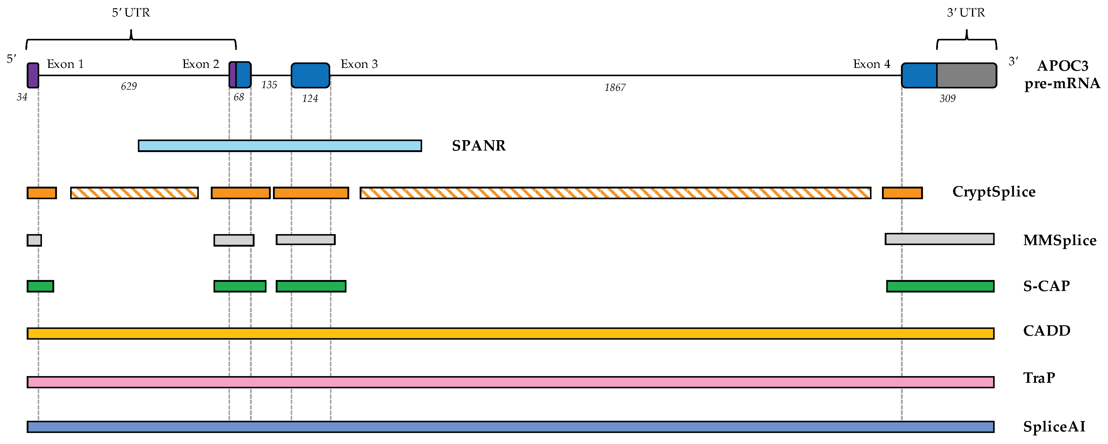
| Tool | Loci Covered |
|---|---|
| SPANR | Any exon that is not first or terminal, plus 300 bp flanking intronic sequence |
| CryptSplice | Within 60 bp of a canonical splice junction; >100 bp into intron if novel donor/acceptor is created |
| MMSplice | Any exon, plus 50 bp upstream or 13 bp downstream |
| S-CAP | Any exon, plus 50 bp flanking intronic sequence |
| CADD | All loci |
| TraP | All loci |
| SpliceAI | All loci |
© 2019 by the authors. Licensee MDPI, Basel, Switzerland. This article is an open access article distributed under the terms and conditions of the Creative Commons Attribution (CC BY) license (http://creativecommons.org/licenses/by/4.0/).
Share and Cite
Rowlands, C.F.; Baralle, D.; Ellingford, J.M. Machine Learning Approaches for the Prioritization of Genomic Variants Impacting Pre-mRNA Splicing. Cells 2019, 8, 1513. https://doi.org/10.3390/cells8121513
Rowlands CF, Baralle D, Ellingford JM. Machine Learning Approaches for the Prioritization of Genomic Variants Impacting Pre-mRNA Splicing. Cells. 2019; 8(12):1513. https://doi.org/10.3390/cells8121513
Chicago/Turabian StyleRowlands, Charlie F, Diana Baralle, and Jamie M Ellingford. 2019. "Machine Learning Approaches for the Prioritization of Genomic Variants Impacting Pre-mRNA Splicing" Cells 8, no. 12: 1513. https://doi.org/10.3390/cells8121513
APA StyleRowlands, C. F., Baralle, D., & Ellingford, J. M. (2019). Machine Learning Approaches for the Prioritization of Genomic Variants Impacting Pre-mRNA Splicing. Cells, 8(12), 1513. https://doi.org/10.3390/cells8121513