Past and Projected Weather Pattern Persistence with Associated Multi-Hazards in the British Isles

 ,
,
Abstract
:1. Introduction
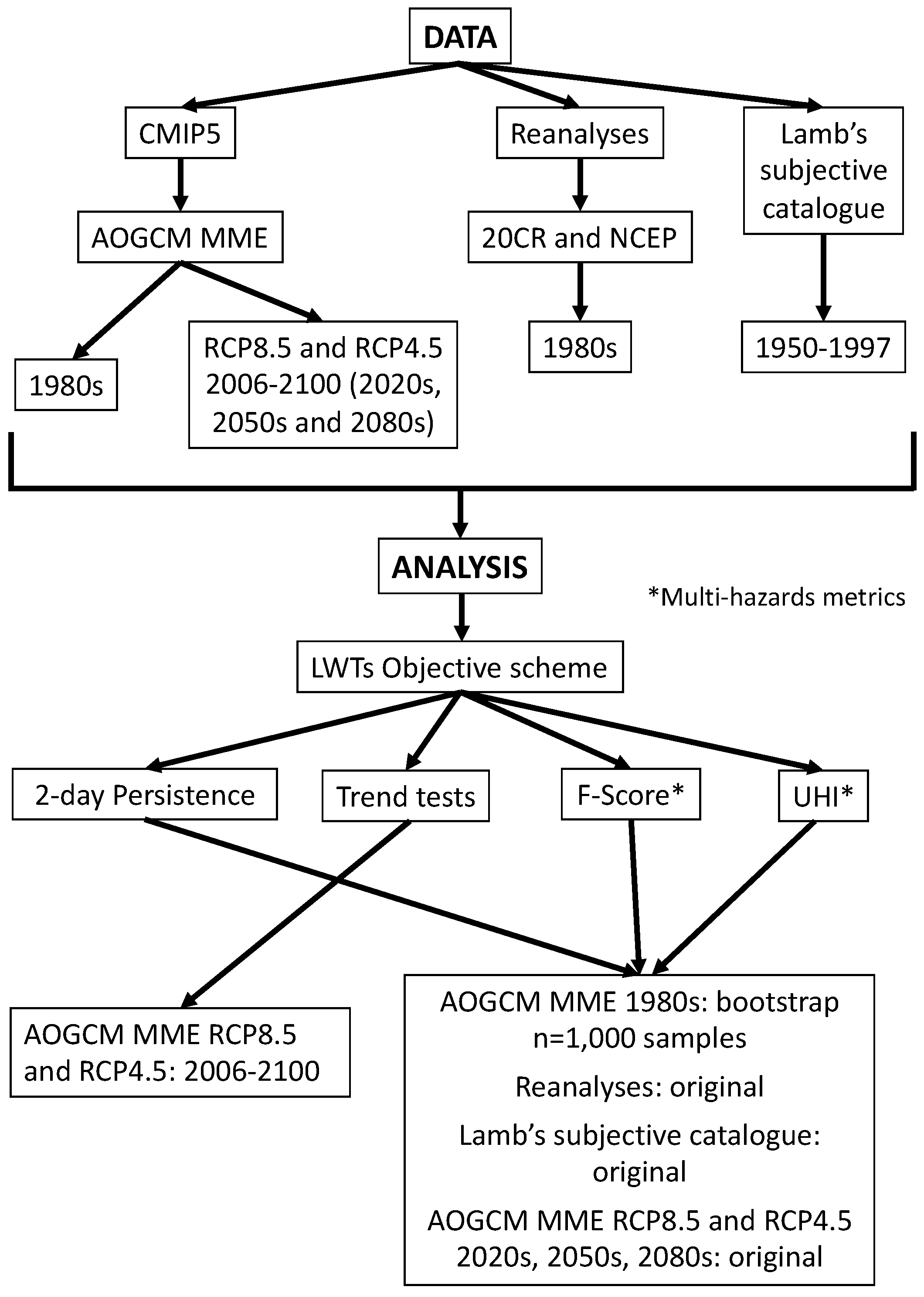
2. Methods and Data
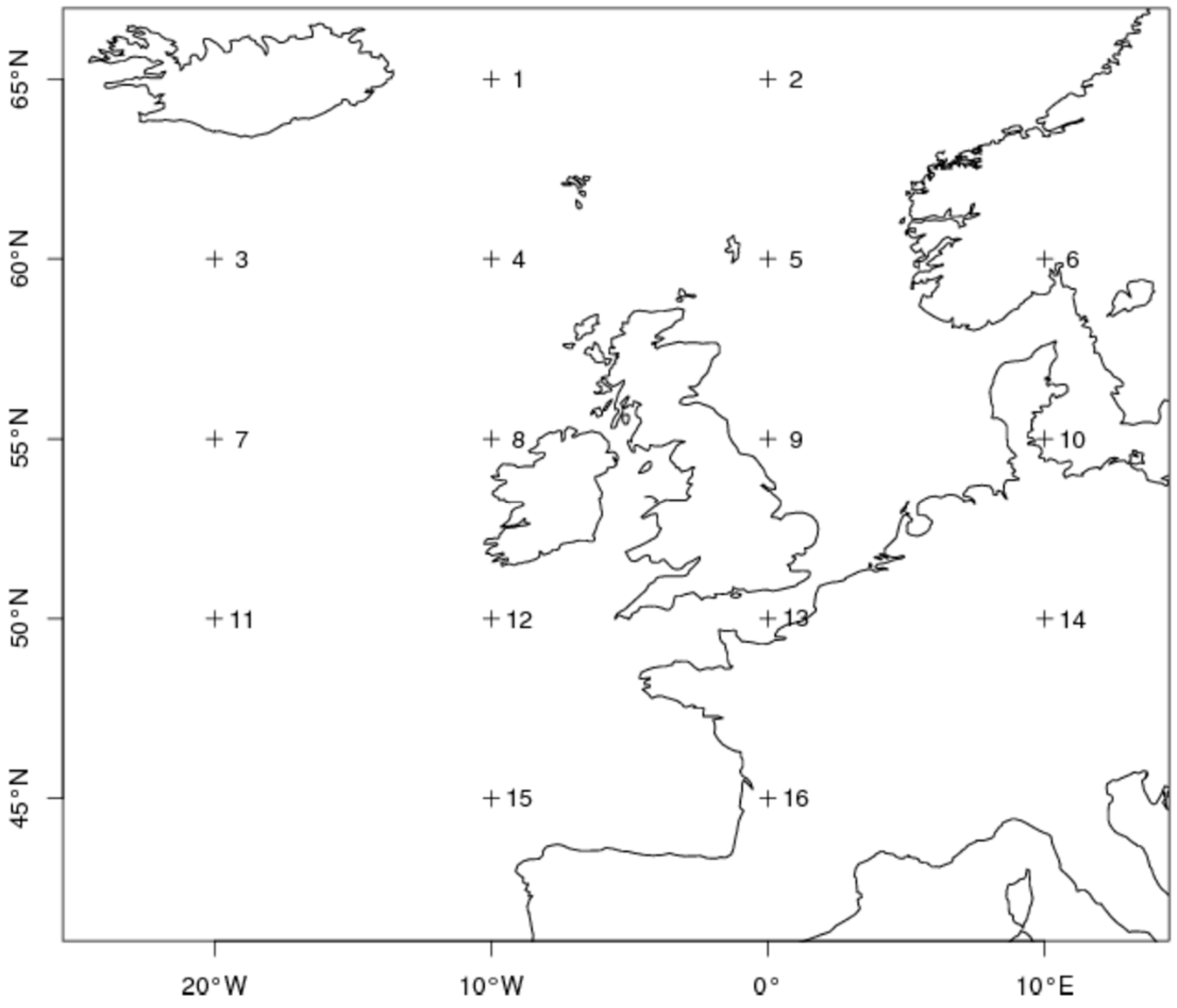
2.1. Lamb Weather Types (LWTs)
- Flow direction is given by tan−1(W/S) and is calculated on an eight-point compass with 45° per sector. If W is positive, add 180°. Thus, the W-type occurs between 247.5° and 292.5° (Equations (1) and (2));
- Lamb pure directional weather types (e.g., N, S, or E-types) correspond to an essentially straight flow, when |Z| is less than F (Equation (6));
- Lamb’s pure cyclonic (C) and anticyclonic (A) types are identified when |Z| is greater than 2F, respectively with Z > 0 and Z < 0 (Equations (3) and (6));
- Lamb’s hybrid types (e.g., AE and CSW) are characterised by a flow partially anticyclonic/cyclonic, with |Z| lying between F and 2F (Equations (3) and (6));
- An unclassified (U) type is obtained when F and |Z| are less than 6, with the choice of 6 depending on grid spacing, meaning that if using a grid resolution finer than 5° by 10° latitude-longitude it needs to be tuned (Equations (3) and (6)).
2.2. Data
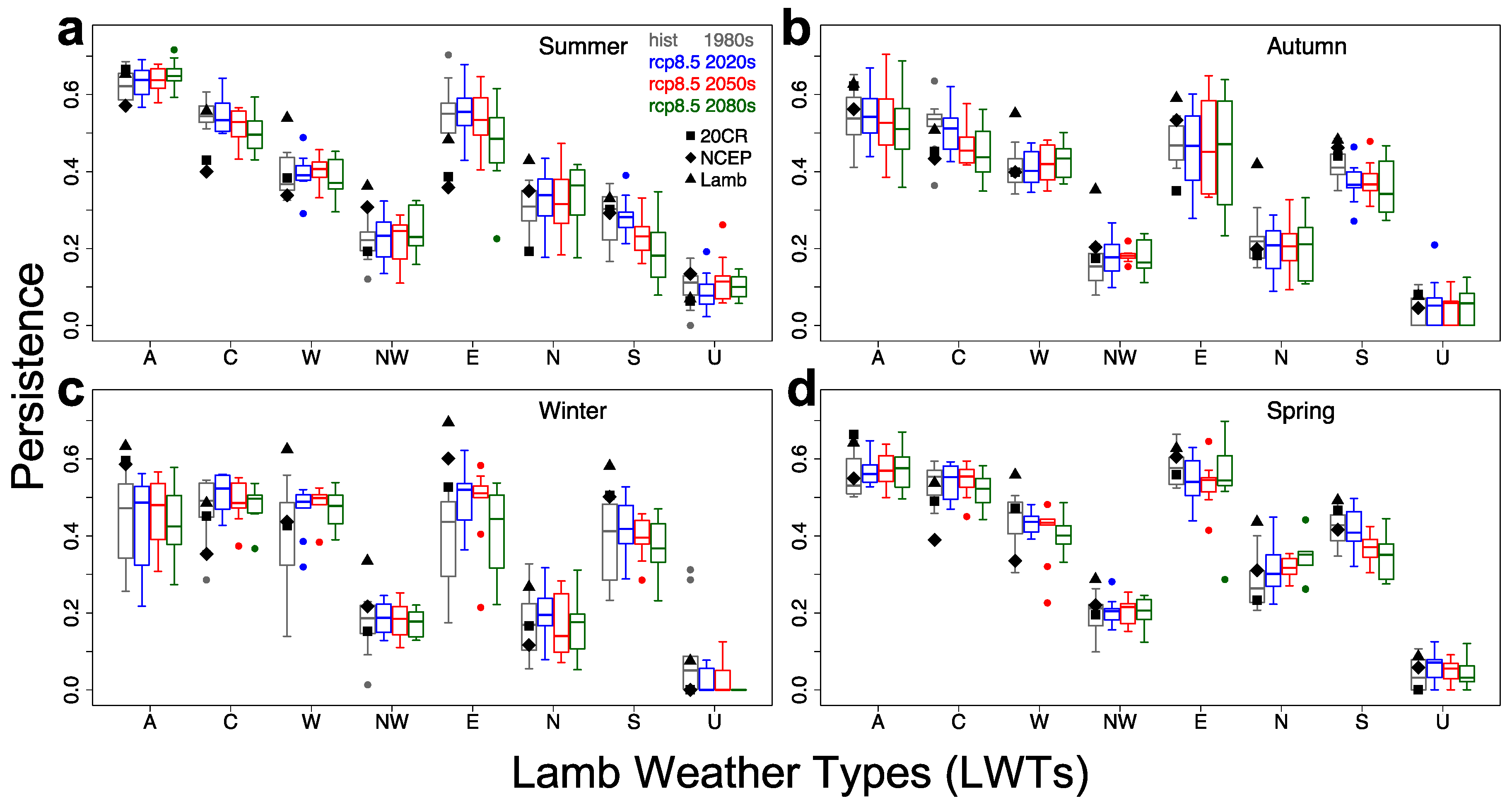
2.3. Persistence and Trend Analyses
2.4. Indices of Winter Fluvial Flooding-Wind Hazards and Summer UHI Intensity
3. Results
3.1. Persistence of Weather Patterns (MME)
3.2. Persistence of Weather Patterns (AOGCMs)
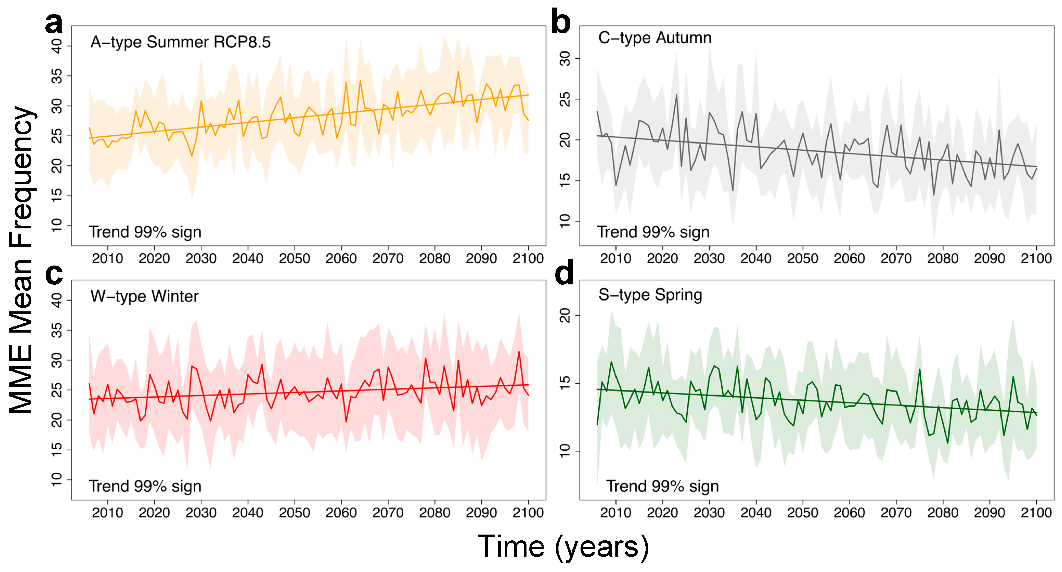
3.3. Frequency of Weather Patterns (MMEM)
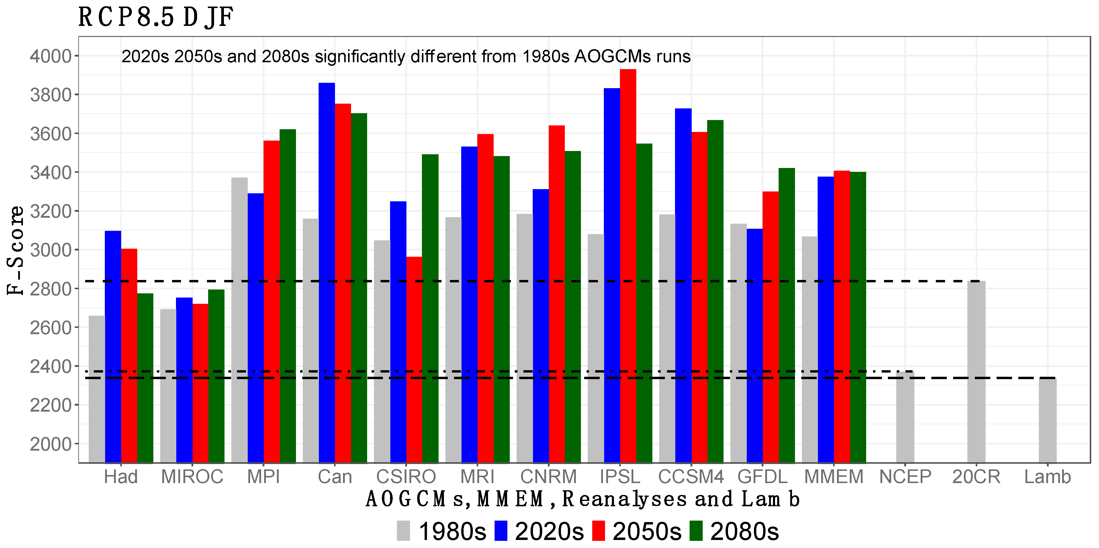
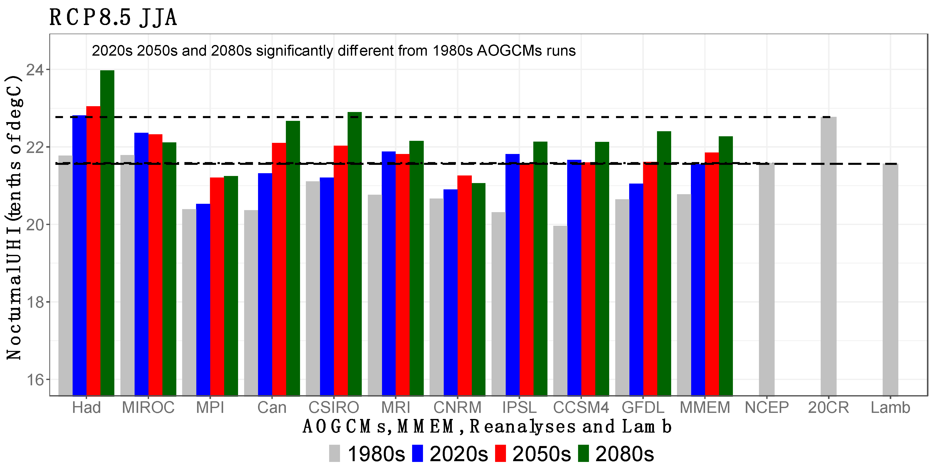
3.4. Application to Future Multi-Hazards
4. Discussion and Conclusions
Supplementary Materials
Author Contributions
Funding
Conflicts of Interest
References
- Coumou, D.; Di Capua, G.; Vavrus, S.; Wang, L.; Wang, S. The influence of Arctic amplification on mid-latitude summer circulation. Nat. Commun. 2018, 9, 2959. [Google Scholar] [CrossRef] [PubMed]
- Francis, J.; Skific, N. Evidence linking rapid Arctic warming to mid-latitude weather patterns. Philos. Trans. R. Soc. A Math. Phys. Eng. Sci. 2015, 373. [Google Scholar] [CrossRef]
- Francis, J.A.; Vavrus, S.J. Evidence linking Arctic amplification to extreme weather in mid-latitudes. Geophys. Res. Lett. 2012, 39. [Google Scholar] [CrossRef]
- Francis, J.A.; Vavrus, S.J. Evidence for a wavier jet stream in response to rapid Arctic warming. Environ. Res. Lett. 2015, 10, 14005. [Google Scholar]
- Munich, R.E. Natural Catastrophes 2014: Analyses, Assessments, Positions; Munich Re: Munich, Germany, 2015. [Google Scholar]
- Munich, Re. NatCatSERVICE—Natural Catastrophes in 2018; Munich Re: Munich, Germany, 2019. [Google Scholar]
- Stott, P.A.; Stone, D.A.; Allen, M.R. Human contribution to the European heatwave of 2003. Nature 2004, 432, 610–614. [Google Scholar] [CrossRef] [PubMed]
- Barriopedro, D.; Fischer, E.M.; Luterbacher, J.; Trigo, R.M.; García-Herrera, R. The Hot Summer of 2010: Redrawing the Temperature Record Map of Europe. Science 2011, 332, 220–224. [Google Scholar] [CrossRef] [PubMed] [Green Version]
- Bastos, A.; Gouveia, C.M.; Trigo, R.M.; Running, S.W. Analysing the spatio-temporal impacts of the 2003 and 2010 extreme heatwaves on plant productivity in Europe. Biogeosciences 2014, 11, 3421–3435. [Google Scholar] [CrossRef] [Green Version]
- Le Tertre, A.; Lefranc, A.; Eilstein, D.; Declercq, C.; Medina, S.; Blanchard, M.; Chardon, B.; Fabre, P.; Filleul, L.; Jusot, J.F.; et al. Impact of the 2003 Heatwave on All-Cause Mortality in 9 French Cities. Epidemiology 2006, 17, 75–79. [Google Scholar]
- Sun, Y.; Zhang, X.; Zwiers, F.W.; Song, L.; Wan, H.; Hu, T.; Yin, H.; Ren, G. Rapid increase in the risk of extreme summer heat in Eastern China. Nat. Clim. Chang. 2014, 4, 1082. [Google Scholar]
- Muchan, K.; Lewis, M.; Hannaford, J.; Parry, S. The winter storms of 2013/2014 in the UK: Hydrological responses and impacts. Weather 2015, 70, 55–61. [Google Scholar] [CrossRef]
- Kendon, M.; McCarthy, M. The UK’s wet and stormy winter of 2013/2014. Weather 2015, 70, 40–47. [Google Scholar] [CrossRef]
- Matthews, T.; Murphy, C.; Wilby, R.L.; Harrigan, S. Stormiest winter on record for Ireland and UK. Nat. Clim. Chang. 2014, 4, 738–740. [Google Scholar] [CrossRef]
- Zscheischler, J.; Westra, S.; Van Den Hurk, B.J.; Seneviratne, S.I.; Ward, P.J.; Pitman, A.; AghaKouchak, A.; Bresch, D.N.; Leonard, M.; Wahl, T.; et al. Future climate risk from compound events. Nat. Clim. Chang. 2018, 8, 469–477. [Google Scholar] [CrossRef]
- AghaKouchak, A.; Huning, L.S.; Chiang, F.; Sadegh, M.; Vahedifard, F.; Mazdiyasni, O.; Moftakhari, H.; Mallakpour, I. How do natural hazards cascade to cause disasters? Nature 2018, 561, 458–460. [Google Scholar] [CrossRef] [PubMed] [Green Version]
- Gill, J.C.; Malamud, B.D. Reviewing and visualizing the interactions of natural hazards. Rev. Geophys. 2014, 52, 680–722. [Google Scholar] [CrossRef] [Green Version]
- Kappes, M.S.; Keiler, M.; von Elverfeldt, K.; Glade, T. Challenges of analyzing multi-hazard risk: A review. Nat. Hazards 2012, 64, 1925–1958. [Google Scholar] [CrossRef]
- Terzi, S.; Torresan, S.; Schneiderbauer, S.; Critto, A.; Zebisch, M.; Marcomini, A. Multi-risk assessment in mountain regions: A review of modelling approaches for climate change adaptation. J. Environ. Manag. 2019, 232, 759–771. [Google Scholar] [CrossRef]
- Forzieri, G.; Feyen, L.; Russo, S.; Vousdoukas, M.; Alfieri, L.; Outten, S.; Migliavacca, M.; Bianchi, A.; Rojas, R.; Cid, A. Multi-hazard assessment in Europe under climate change. Clim. Chang. 2016, 137, 105–119. [Google Scholar] [CrossRef] [Green Version]
- Gallina, V.; Torresan, S.; Critto, A.; Sperotto, A.; Glade, T.; Marcomini, A. A review of multi-risk methodologies for natural hazards: Consequences and challenges for a climate change impact assessment. J. Environ. Manag. 2016, 168, 123–132. [Google Scholar]
- UNDRR. Sendai Framework for Disaster Risk Reduction 2015–2030; UNDRR: Geneva, Switzerland, 2015. [Google Scholar]
- Leonard, M.; Westra, S.; Phatak, A.; Lambert, M.; van den Hurk, B.; McInnes, K.; Risbey, J.; Schuster, S.; Jakob, D.; Stafford-Smith, M. A compound event framework for understanding extreme impacts. Wiley Interdiscip. Rev. Clim. Chang. 2014, 5, 113–128. [Google Scholar] [CrossRef]
- Kargel, J.S.; Leonard, G.J.; Shugar, D.H.; Haritashya, U.K.; Bevington, A.; Fielding, E.J.; Fujita, K.; Geertsema, M.; Miles, E.S.; Steiner, J.; et al. Geomorphic and geologic controls of geohazards induced by Nepal’s 2015 Gorkha earthquake. Science 2016, 351, aac8353. [Google Scholar] [PubMed]
- De Luca, P.; Hillier, J.K.; Wilby, R.L.; Quinn, N.W.; Harrigan, S. Extreme multi-basin flooding linked with extra-tropical cyclones. Environ. Res. Lett. 2017, 12, 114009. [Google Scholar] [CrossRef]
- Ward, P.J.; Couasnon, A.; Eilander, D.; Haigh, I.D.; Hendry, A.; Muis, S.; Veldkamp, T.I.; Winsemius, H.C.; Wahl, T. Dependence between high sea-level and high river discharge increases flood hazard in global deltas and estuaries. Environ. Res. Lett. 2018, 13, 84012. [Google Scholar] [CrossRef]
- Bevacqua, E.; Maraun, D.; Vousdoukas, M.I.; Voukouvalas, E.; Vrac, M.; Mentaschi, L.; Widmann, M. Higher probability of compound flooding from precipitation and storm surge in Europe under anthropogenic climate change. Sci. Adv. 2019, 5, eaaw5531. [Google Scholar] [CrossRef] [Green Version]
- Khanal, S.; Ridder, N.; de Vries, H.; Terink, W.; van den Hurk, B. Storm Surge and Extreme River Discharge: A Compound Event Analysis Using Ensemble Impact Modeling. Front. Earth Sci. 2019, 7, 224. [Google Scholar] [CrossRef]
- Collet, L.; Harrigan, S.; Prudhomme, C.; Formetta, G.; Beevers, L. Future hot-spots for hydro-hazards in Great Britain: A probabilistic assessment. Hydrol. Earth Syst. Sci. 2018, 22, 5387–5401. [Google Scholar] [CrossRef]
- De Luca, P.; Messori, G.; Wilby, R.L.; Mazzoleni, M.; Di Baldassarre, G. Concurrent wet and dry hydrological extremes at the global scale. Earth Syst. Dyn. 2019, 1–24. [Google Scholar] [CrossRef]
- Visser-Quinn, A.; Beevers, L.; Collet, L.; Formetta, G.; Smith, K.; Wanders, N.; Thober, S.; Pan, M.; Kumar, R. Spatio-temporal analysis of compound hydro-hazard extremes across the UK. Adv. Water Resour. 2019, 130, 77–90. [Google Scholar] [CrossRef]
- De Luca, P.; Messori, G.; Faranda, D. Dynamical Systems Theory Sheds New Light on Compound Climate Extremes in Europe and Eastern North America. EarthArXiv 2019. [Google Scholar] [CrossRef] [Green Version]
- Lamb, H.H. British Isles Weather Types and a Register of Daily Sequence of Circulation Patterns, 1861–1971; Geophysical Memoir 116; HMSO: London, UK, 1972.
- Jenkinson, A.F.; Collison, F.P. An Initial Climatology of Gales over the North Sea; Synoptic Climatology Branch Memorandum No. 62; Meteorological Office: Bracknell, UK, 1977.
- Jones, P.D.; Hulme, M.; Briffa, K.R. A comparison of Lamb circulation types with an objective classification scheme. Int. J. Climatol. 1993, 13, 655–663. [Google Scholar] [CrossRef]
- Jones, P.D.; Harpham, C.; Briffa, K.R. Lamb weather types derived from reanalysis products. Int. J. Climatol. 2013, 33, 1129–1139. [Google Scholar] [CrossRef]
- Jones, P.D.; Osborn, T.J.; Harpham, C.; Briffa, K.R. The development of Lamb weather types: From subjective analysis of weather charts to objective approaches using reanalyses. Weather 2014, 69, 128–132. [Google Scholar] [CrossRef]
- Wilby, R.L.; Jones, P.D.; Lister, D.H. Decadal variations in the nocturnal heat island of London. Weather 2011, 66, 59–64. [Google Scholar] [CrossRef]
- Merz, B.; Aerts, J.C.; Arnbjerg-Nielsen, K.; Baldi, M.; Becker, A.; Bichet, A.; Blöschl, G.; Bouwer, L.M.; Brauer, A.; Cioffi, F.; et al. Floods and climate: Emerging perspectives for flood risk assessment and management. Nat. Hazards Earth Syst. Sci. 2014, 14, 1921–1942. [Google Scholar] [CrossRef]
- Conticello, F.; Cioffi, F.; Merz, B.; Lall, U. An event synchronization method to link heavy rainfall events and large-scale atmospheric circulation features. Int. J. Climatol. 2018, 38, 1421–1437. [Google Scholar] [CrossRef]
- Farnham, D.J.; Doss-Gollin, J.; Lall, U. Regional Extreme Precipitation Events: Robust Inference From Credibly Simulated GCM Variables. Water Resour. Res. 2018, 54, 3809–3824. [Google Scholar] [CrossRef]
- Murawski, A.; Vorogushyn, S.; Bürger, G.; Gerlitz, L.; Merz, B. Do Changing Weather Types Explain Observed Climatic Trends in the Rhine Basin? An Analysis of Within- and Between-Type Changes. J. Geophys. Res. Atmos. 2018, 123, 1562–1584. [Google Scholar] [CrossRef]
- Murawski, A.; Bürger, G.; Vorogushyn, S.; Merz, B. Can local climate variability be explained by weather patterns? A multi-station evaluation for the Rhine basin. Hydrol. Earth Syst. Sci. 2016, 20, 4283–4306. [Google Scholar] [CrossRef] [Green Version]
- Pattison, I.; Lane, S.N. The relationship between Lamb weather types and long-term changes in flood frequency, River Eden, UK. Int. J. Climatol. 2012, 32, 1971–1989. [Google Scholar] [CrossRef]
- Matthews, T.; Murphy, C.; Wilby, R.L.; Harrigan, S. A cyclone climatology of the British-Irish Isles 1871–2012. Int. J. Climatol. 2016, 36, 1299–1312. [Google Scholar] [CrossRef]
- Ridder, N.; de Vries, H.; Drijfhout, S. The role of atmospheric rivers in compound events consisting of heavy precipitation and high storm surges along the Dutch coast. Nat. Hazards Earth Syst. Sci. 2018, 18, 3311–3326. [Google Scholar] [CrossRef] [Green Version]
- Wilby, R.L.; Wigley, T.M.L. Downscaling general circulation model output: A review of methods and limitations. Prog. Phys. Geogr. Earth Environ. 1997, 21, 530–548. [Google Scholar] [CrossRef]
- Xu, H.; Corte-Real, J.; Qian, B. Developing daily precipitation scenarios for climate change impact studies in the Guadiana and the Tejo basins. Hydrol. Earth Syst. Sci. 2007, 11, 1161–1173. [Google Scholar] [CrossRef]
- Wilby, R.L.; Quinn, N.W. Reconstructing multi-decadal variations in fluvial flood risk using atmospheric circulation patterns. J. Hydrol. 2013, 487, 109–121. [Google Scholar] [CrossRef]
- Wilby, R.L. Constructing Climate Change Scenarios of Urban Heat Island Intensity and Air Quality. Environ. Plan. B Plan. Des. 2008, 35, 902–919. [Google Scholar] [CrossRef]
- Burt, T.P.; Jones, P.D.; Howden, N.J.K. An analysis of rainfall across the British Isles in the 1870s. Int. J. Climatol. 2015, 35, 2934–2947. [Google Scholar] [CrossRef]
- Tyler, J.J.; Jones, M.; Arrowsmith, C.; Allott, T.; Leng, M.J. Spatial patterns in the oxygen isotope composition of daily rainfall in the British Isles. Clim. Dyn. 2016, 47, 1971–1987. [Google Scholar] [CrossRef]
- Stryhal, J.; Huth, R. Trends in winter circulation over the British Isles and central Europe in twenty-first century projections by 25 CMIP5 GCMs. Clim. Dyn. 2018. [Google Scholar] [CrossRef]
- Otero, N.; Sillmann, J.; Butler, T. Assessment of an extended version of the Jenkinson–Collison classification on CMIP5 models over Europe. Clim. Dyn. 2018, 50, 1559–1579. [Google Scholar] [CrossRef]
- Pope, R.J.; Butt, E.W.; Chipperfield, M.P.; Doherty, R.M.; Fenech, S.; Schmidt, A.; Arnold, S.R.; Savage, N.H. The impact of synoptic weather on UK surface ozone and implications for premature mortality. Environ. Res. Lett. 2016, 11. [Google Scholar] [CrossRef]
- Burt, T.P.; Ferranti, E.J.S. Changing patterns of heavy rainfall in upland areas: A case study from northern England. Int. J. Climatol. 2012, 32, 518–532. [Google Scholar] [CrossRef]
- Jones, P.D.; Harpham, C.; Lister, D. Long-term trends in gale days and storminess for the Falkland Islands. Int. J. Climatol. 2016, 36, 1413–1427. [Google Scholar] [CrossRef]
- Wetterhall, F.; Pappenberger, F.; He, Y.; Freer, J.; Cloke, H.L. Conditioning model output statistics of regional climate model precipitation on circulation patterns. Nonlinear Process. Geophys. 2012, 19, 623–633. [Google Scholar] [CrossRef] [Green Version]
- Richardson, D.; Fowler, H.J.; Kilsby, C.G.; Neal, R. A new precipitation and drought climatology based on weather patterns. Int. J. Climatol. 2018, 38, 630–648. [Google Scholar] [CrossRef] [PubMed]
- Wilby, R.L.; Dalgleish, H.Y.; Foster, I.D.L. The impact of weather patterns on historic and contemporary catchment sediment yields. Earth Surf. Process. Landf. 1997, 22, 353–363. [Google Scholar]
- Blenkinsop, S.; Chan, S.C.; Kendon, E.J.; Roberts, N.M.; Fowler, H.J. Temperature influences on intense UK hourly precipitation and dependency on large-scale circulation. Environ. Res. Lett. 2015, 10, 54021. [Google Scholar] [CrossRef]
- Fowler, H.J.; Kilsby, C.G. A weather-type approach to analysing water resource drought in the Yorkshire region from 1881 to 1998. J. Hydrol. 2002, 262, 177–192. [Google Scholar] [CrossRef]
- Wilby, R.L. The influence of variable weather patterns on river water quantity and quality regimes. Int. J. Climatol. 1993, 13, 447–459. [Google Scholar] [CrossRef]
- Tang, L.; Chen, D.; Karlsson, P.; Gu, Y.; Ou, T. Synoptic circulation and its influence on spring and summer surface ozone concentrations in southern Sweden. Boreal Environ. Res. 2009, 14, 889–902. [Google Scholar]
- Grundström, M.; Hak, C.; Chen, D.; Hallquist, M.; Pleijel, H. Variation and co-variation of PM10, particle number concentration, NOx and NO2 in the urban air—Relationships with wind speed, vertical temperature gradient and weather type. Atmos. Environ. 2015, 120, 317–327. [Google Scholar] [CrossRef]
- Cortesi, N.; Gonzalez-Hidalgo, J.C.; Trigo, R.M.; Ramos, A.M. Weather types and spatial variability of precipitation in the Iberian Peninsula. Int. J. Climatol. 2014, 34, 2661–2677. [Google Scholar] [CrossRef]
- Domínguez-Castro, F.; Ramos, A.M.; García-Herrera, R.; Trigo, R.M. Iberian extreme precipitation 1855/1856: An analysis from early instrumental observations and documentary sources. Int. J. Climatol. 2015, 35, 142–153. [Google Scholar] [CrossRef]
- Eiras-Barca, J.; Lorenzo, N.; Taboada, J.; Robles, A.; Miguez-Macho, G. On the relationship between atmospheric rivers, weather types and floods in Galicia (NW Spain). Nat. Hazards Earth Syst. Sci. 2018, 18, 1633–1645. [Google Scholar] [CrossRef] [Green Version]
- Lorenzo, M.N.; Taboada, J.J.; Gimeno, L. Links between circulation weather types and teleconnection patterns and their influence on precipitation patterns in Galicia (NW Spain). Int. J. Climatol. 2008, 28, 1493–1505. [Google Scholar] [CrossRef]
- Woollings, T.; Barriopedro, D.; Methven, J.; Son, S.W.; Martius, O.; Harvey, B.; Sillmann, J.; Lupo, A.R.; Seneviratne, S. Blocking and its Response to Climate Change. Curr. Clim. Chang. Rep. 2018. [Google Scholar] [CrossRef]
- Taylor, K.E.; Stouffer, R.J.; Meehl, G.A. An Overview of CMIP5 and the Experiment Design. Bull. Am. Meteorol. Soc. 2011, 93, 485–498. [Google Scholar] [CrossRef]
- Compo, G.P.; Whitaker, J.S.; Sardeshmukh, P.D.; Matsui, N.; Allan, R.J.; Yin, X.; Gleason, B.E.; Vose, R.S.; Rutledge, G.; Bessemoulin, P.; et al. The Twentieth Century Reanalysis Project. Q. J. R. Meteorol. Soc. 2011, 137, 1–28. [Google Scholar] [CrossRef]
- Kalnay, E.; Kanamitsu, M.; Kistler, R.; Collins, W.; Deaven, D.; Gandin, L.; Iredell, M.; Saha, S.; White, G.; Woollen, J.; et al. The NCEP/NCAR 40-Year Reanalysis Project. Bull. Am. Meteorol. Soc. 1996, 77, 437–471. [Google Scholar] [CrossRef]
- Hulme, M.; Barrow, E. Climate of the British Isles: Present, Past and Future; Routledge: London, UK, 1997. [Google Scholar]
- Jones, P.D.; Kelly, P.M. Principal component analysis of the Lamb Catalogue of Daily Weather Types: Part 1, annual frequencies. Int. J. Climatol. 1982, 2, 147–157. [Google Scholar]
- Lamb, H.H. Types and spells of weather around the year in the British Isles: Annual trends, seasonal structure of the year, singularities. Q. J. R. Meteorol. Soc. 1950, 76, 393–429. [Google Scholar] [CrossRef]
- Hulme, M.; Briffa, K.R.; Jones, P.D.; Senior, C.A. Validation of GCM control simulations using indices of daily airflow types over the British Isles. Clim. Dyn. 1993, 9, 95–105. [Google Scholar] [CrossRef]
- Diaz-Nieto, J.; Wilby, R.L. A comparison of statistical downscaling and climate change factor methods: Impacts on low flows in the River Thames, United Kingdom. Clim. Chang. 2005, 69, 245–268. [Google Scholar] [CrossRef]
- Li, T.; Horton, R.M.; Kinney, P.L. Projections of seasonal patterns in temperature-related deaths for Manhattan, New York. Nat. Clim. Chang. 2013, 3, 717. [Google Scholar] [PubMed]
- Dolinar, E.K.; Dong, X.; Xi, B. Evaluation and intercomparison of clouds, precipitation, and radiation budgets in recent reanalyses using satellite-surface observations. Clim. Dyn. 2016, 46, 2123–2144. [Google Scholar] [CrossRef]
- Decker, M.; Brunke, M.A.; Wang, Z.; Sakaguchi, K.; Zeng, X.; Bosilovich, M.G. Evaluation of the Reanalysis Products from GSFC, NCEP, and ECMWF Using Flux Tower Observations. J. Clim. 2011, 25, 1916–1944. [Google Scholar] [CrossRef]
- Wilby, R.L. Stochastic weather type simulation for regional climate change impact assessment. Water Resour. Res. 1994, 30, 3395–3403. [Google Scholar] [CrossRef]
- Gagniuc, P.A. Markov Chains: From Theory to Implementation and Experimentation; John Wiley & Sons: Hoboken, NJ, USA, 2017. [Google Scholar] [CrossRef]
- Spedicato, G.A. Discrete Time Markov Chains with R. R J. 2017, 9, 84–104. [Google Scholar]
- Mann, H.B.; Whitney, D.R. On a Test of Whether one of Two Random Variables is Stochastically Larger than the Other. Ann. Math. Stat. 1947, 18, 50–60. [Google Scholar] [CrossRef]
- Hamed, K.H.; Ramachandra Rao, A. A modified Mann-Kendall trend test for autocorrelated data. J. Hydrol. 1998, 204, 182–196. [Google Scholar] [CrossRef]
- Sen, P.K. Estimates of the Regression Coefficient Based on Kendall’s Tau. J. Am. Stat. Assoc. 1968, 63, 1379–1389. [Google Scholar] [CrossRef]
- O’Hare, G.P.P.; Wilby, R.L. A Review of Ozone Pollution in the United Kingdom and Ireland with an Analysis Using Lamb Weather Types. Geogr. J. 1995, 161, 1–20. [Google Scholar] [CrossRef]
- Pope, R.J.; Savage, N.H.; Chipperfield, M.P.; Arnold, S.R.; Osborn, T.J. The influence of synoptic weather regimes on UK air quality: Analysis of satellite column NO2. Atmos. Sci. Lett. 2014, 15, 211–217. [Google Scholar] [CrossRef]
- Tang, Q.; Zhang, X.; Francis, J.A. Extreme summer weather in northern mid-latitudes linked to a vanishing cryosphere. Nat. Clim. Chang. 2013, 4, 45. [Google Scholar]
- Pfleiderer, P.; Schleussner, C.F.; Kornhuber, K.; Coumou, D. Summer weather becomes more persistent in a 2 °C world. Nat. Clim. Chang. 2019. [Google Scholar] [CrossRef]
- Screen, J.A.; Simmonds, I. The central role of diminishing sea ice in recent Arctic temperature amplification. Nature 2010, 464, 1334. [Google Scholar] [PubMed]
- Cohen, J.; Screen, J.A.; Furtado, J.C.; Barlow, M.; Whittleston, D.; Coumou, D.; Francis, J.; Dethloff, K.; Entekhabi, D.; Overland, J.; et al. Recent Arctic amplification and extreme mid-latitude weather. Nat. Geosci. 2014, 7, 627. [Google Scholar] [CrossRef]
- Francis, J.A. Why Are Arctic Linkages to Extreme Weather Still up in the Air? Bull. Am. Meteorol. Soc. 2017, 98, 2551–2557. [Google Scholar] [CrossRef]
- Francis, J.A.; Vavrus, S.J.; Cohen, J. Amplified Arctic warming and mid-latitude weather: New perspectives on emerging connections. Wiley Interdiscip. Rev. Clim. Chang. 2017, 8, e474. [Google Scholar] [CrossRef]
- Barnes, E.A. Revisiting the evidence linking Arctic amplification to extreme weather in midlatitudes. Geophys. Res. Lett. 2013, 40, 4734–4739. [Google Scholar] [CrossRef]
- Woollings, T.; Harvey, B.; Masato, G. Arctic warming, atmospheric blocking and cold European winters in CMIP5 models. Environ. Res. Lett. 2014, 9, 14002. [Google Scholar] [CrossRef]
- Burt, T.P.; Howden, N.J.K. North Atlantic Oscillation amplifies orographic precipitation and river flow in upland Britain. Water Resour. Res. 2013, 49, 3504–3515. [Google Scholar] [CrossRef]
- Murphy, J.M.; Sexton, D.M.; Jenkins, G.J.; Boorman, P.M.; Booth, B.B.; Brown, C.C.; Clark, R.T.; Collins, M.; Harris, G.R.; Kendon, E.J.; et al. UK Climate Projections Science Report: Climate Change Projections; Met Office Hadley Centre: Exeter, UK, 2009.
- Hess, P.; Brezowsky, H. Katalog der Großwetterlagen Europas. In Berichte des Deutschen Wetterdienstes in der US-Zone 33; DeutscherWetterdienst in der US-Zone: Bad Kissingen, Germany, 1952. [Google Scholar]
- Prein, A.F.; Bukovsky, M.S.; Mearns, L.O.; Bruyère, C.L.; Done, J.M. Simulating North American Weather Types With Regional Climate Models. Front. Environ. Sci. 2019, 7, 36. [Google Scholar] [CrossRef]
- Kalkstein, L.S.; Nichols, M.C.; Barthel, C.D.; Greene, J.S. A new spatial synoptic classification: Application to air-mass analysis. Int. J. Climatol. 1996, 16, 983–1004. [Google Scholar] [CrossRef]


| LWT | Description |
|---|---|
| Anticyclonic (A) | Anticyclones centred over, near, or extending over the British Isles. |
| Cyclonic (C) | Depressions passing frequently or stagnating over the British Isles. The central isobar of the depression should extend over the mainland of Britain or Ireland. |
| Westerly (W) | High pressure to the south and low pressure to the north, giving a sequence of depressions travelling eastward across the Atlantic. This is the main, progressive zonal type. |
| North-westerly (NW) | Azores anticyclone displaced northeast or north towards the British Isles. Depressions forming near Iceland and travelling south-east into the North Sea. |
| Easterly (E) | Anticyclones over Scandinavia extending towards Iceland across the Norwegian Sea. Depressions generally to the south of the region over south-west Europe and the western Atlantic. |
| Northerly (N) | High pressure to the west or northwest of Britain extending from Greenland southwards, possibly as far as the Azores. Depressions travel southward from the Norwegian Sea. |
| Southerly (S) | High pressure over central and northern Europe. Depressions blocked to the west or travelling north or north-eastwards off western coasts. |
| Unclassified (U) | Weather pattern weak or chaotic. |
| Model Name | Research Institute | Lat-Lon Resolution | Ensemble Member |
|---|---|---|---|
| HadGEM2-ES | Met Office, United Kingdom | 1.25° × 1.875° | r1i1p1 |
| MPI-ESM-LR | Max Planck Institute for Meteorology, Germany | 1.9° × 1.9° | r1i1p1 |
| MRI-CGCM3 | Meteorological Research Institute, Japan | 1.1° × 1.1° | r1i1p1 |
| CNRM-CM5 | National Centre for Meteorological Research, France | 1.4° × 1.4° | r1i1p1 |
| CanESM2 | Canadian Center for Climate Modeling and Analysis, Canada | 2.8° × 2.8° | r1i1p1 |
| MIROC5 | Model for Interdisciplinary Research on Climate, Japan | 1.4° × 1.4° | r1i1p1 |
| CSIRO-Mk3.6.0 | Commonwealth Scientific and Industrial Research Organisation, Australia | 1.9° × 1.9° | r10i1p1 |
| IPSL-CM5A-LR | Institute Pierre-Simon Laplace, France | 1.9° × 3.75° | r1i1p1 |
| CCSM4 | National Center for Atmospheric Research, USA | 0.94° × 1.25° | r6i1p1 |
| GFDL-CM3 | Geophysical Fluid Dynamics Laboratory, USA | 2° × 2.5° | r1i1p1 |
© 2019 by the authors. Licensee MDPI, Basel, Switzerland. This article is an open access article distributed under the terms and conditions of the Creative Commons Attribution (CC BY) license (http://creativecommons.org/licenses/by/4.0/).
Share and Cite
De Luca, P.; Harpham, C.; Wilby, R.L.; Hillier, J.K.; Franzke, C.L.E.; Leckebusch, G.C. Past and Projected Weather Pattern Persistence with Associated Multi-Hazards in the British Isles. Atmosphere 2019, 10, 577. https://doi.org/10.3390/atmos10100577
De Luca P, Harpham C, Wilby RL, Hillier JK, Franzke CLE, Leckebusch GC. Past and Projected Weather Pattern Persistence with Associated Multi-Hazards in the British Isles. Atmosphere. 2019; 10(10):577. https://doi.org/10.3390/atmos10100577
Chicago/Turabian StyleDe Luca, Paolo, Colin Harpham, Robert L. Wilby, John K. Hillier, Christian L. E. Franzke, and Gregor C. Leckebusch. 2019. "Past and Projected Weather Pattern Persistence with Associated Multi-Hazards in the British Isles" Atmosphere 10, no. 10: 577. https://doi.org/10.3390/atmos10100577