Statistics of the Optical Turbulence from the Micrometeorological Measurements at the Baykal Astrophysical Observatory Site

Abstract

The paper focuses on the investigations of the optical turbulence structure. The distributions of the repeatability of the structure characteristic of the air refractive index are obtained. A scenario of decreasing the intensity of the optical turbulence in the summer is discussed. Numerical estimates of this scenario are given. Using classical methods of wavefront analysis, the results of the first studies of the vertical structure of atmospheric turbulence at the Baykal astrophysical observatory site are presented.

1. Introduction

The degradation of image quality due to the atmospheric turbulence has been a long-known problem. Turbulent fluctuations of both air temperature and wind speed induce variations in the air refractive index. The study of the atmospheric turbulence and its optical properties is important for astroclimatic research, planning time of astronomical observations as well as searching for the physical mechanisms of its formation. In particular, the study of the surface layer over rough terrain is relevant. In rough terrain, the structure of the turbulence is broken. With wave and vortex disturbances arising, mesoscale airflows may induce the intense turbulence and variations in the exchange of heat, momentum, and mass. The work is aimed at studying the structure of optical turbulence at the Baykal astrophysical observatory site. Statistics of the optical turbulence includes a lot of parameters, some of which are analyzed in [1,2]. We focus on the study of the the main characteristic of the optical turbulence that affects the image quality is the structure characteristic of the air refractive index fluctuations $C_n^2$. The quantity $C_n^2$ is the parameter included in Kolmogorov–Obukhov “$2/3$”-power law:

$$D_n=C_n^2{r}^{2/3},$$

(1)

where n is the air refraction index, $D_n$ is the structure function, and r is the distance between two given points at which the air refraction index is determined.

As the air refraction index fluctuations are related mainly to the air temperature fluctuations, $C_n^2$ is proportional to the structure characteristic of the air temperature fluctuations $C_T^2$:

$$C_n^2={\left(\frac{AP}{<T{>}^2}\right)}^2{C}_T^2,$$

(2)

where A is constant for the light wavelength $\lambda$ ($A=79.3\times {10}^{-6}$ at $\lambda$ = 0.5 $\mathsf{\mu }$m), P—the atmospheric pressure, and $<T>$—averaged air temperature for the given time period. The quantity $C_n^2$ defines the well known Fried radius $r_0$, which described the quality of seeing [3]:

$$r_0={\left(0.423k^{2}sec\alpha \underset{0}{\overset{H}{\int }}{C}_n^2\left(z\right)dz\right)}^{-3/5},$$

(3)

where $\alpha$—zenith angle, $k=2\pi /\lambda$, $\lambda$—the wavelength of the light, $H\sim 20$ km—the height of the “optically active” atmosphere.

In addition, the isoplanatic angle is determined by the vertical profile $C_n^2\left(z\right)$ [3]:

$${\theta }_0={\left(2.91{\left(\frac{2\pi }{\lambda }\right)}^2{sec}^{8/3}\alpha {\int }_0^H{C}_n^2\left(z\right)z^{5/3}dz\right)}^{-3/5}.$$

(4)

In order to improve our knowledge about the statistical properties of turbulent mixing in the atmospheric boundary layer, the exchange of turbulent kinetic and potential energy in the atmosphere as well as optical turbulence, long-period measurements of both the air temperature, and wind speed have been performed.

2. The Repeatability of the Optical Turbulence at the Baykal Astrophysical Observatory Site

To study the atmospheric turbulence, large scale air motions, temporal variations of the mean meteorological characteristics, the data of ultrasonic anemometers are widely used [4,5,6,7,8].The results of a field intercomparison experiment of a number of sonic anemometer models point to biases in the measured characteristics. However, biases are generally very small for these sensors [9]. Comparative statistical analysis of the mean meteorological characteristics measured by the ultrasonic anemometers with data of the lidars and mechanical anemometers shows a very good agreement [6,7,10,11].

To estimate the strength of the optical turbulence in the atmospheric boundary layer at the Baykal astrophysical observatory site, we performed the measurements of the air temperature and wind speed using meteorological weather station “AMK-03” (sonic anemometer) mounted on a mast (Figure 1) [8]. The height of the meteorological weather station above the underlying surface was about 30 m. Using the meteorological weather station “AMK-03” mounted on the mast, we carried out the measurements every day during the time period from 1 January to 31 December 2018. The estimations of the air temperature and components of the wind speed are based on the dependence of the group speed of sound in the atmosphere on the air temperature. The data allow us to obtain long period time series of the air temperature and wind speed measured with high sampling rate (10 Hz). Initial averaging of the air temperature, the structure characteristic of the air temperature fluctuations and the structure characteristic of the air refractive index fluctuations was performed every 3 min. The time interval between two measurements was 10 min. The total amount of accumulated data are about 17,000 values of averaged structure characteristic of the air refractive index fluctuations during the year. Using time series recorded, we assess mean air temperature $<T>$ and $C_n^2$ using a standard approach [7].

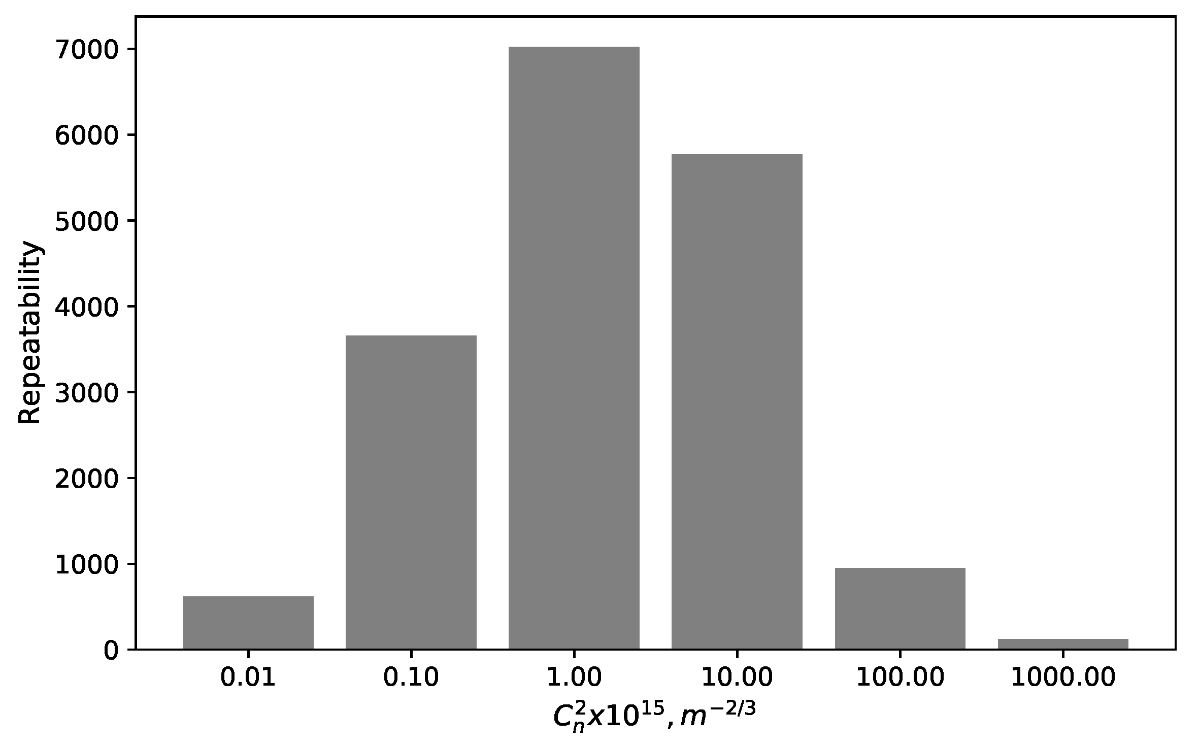
The distribution of the repeatability of the structure characteristic of the air refractive index fluctuations for the period from from 1 January to 31 December 2018 is shown in Figure 2.

It is important that there is a significant asymmetry in the repeatability of $C_n^2$. The atmospheric boundary layer at the Baykal astrophysical observatory site is characterized by a moderate turbulence. The values of $C_n^2$ often exceed ${10}^{-14}{m}^{-2/3}$.

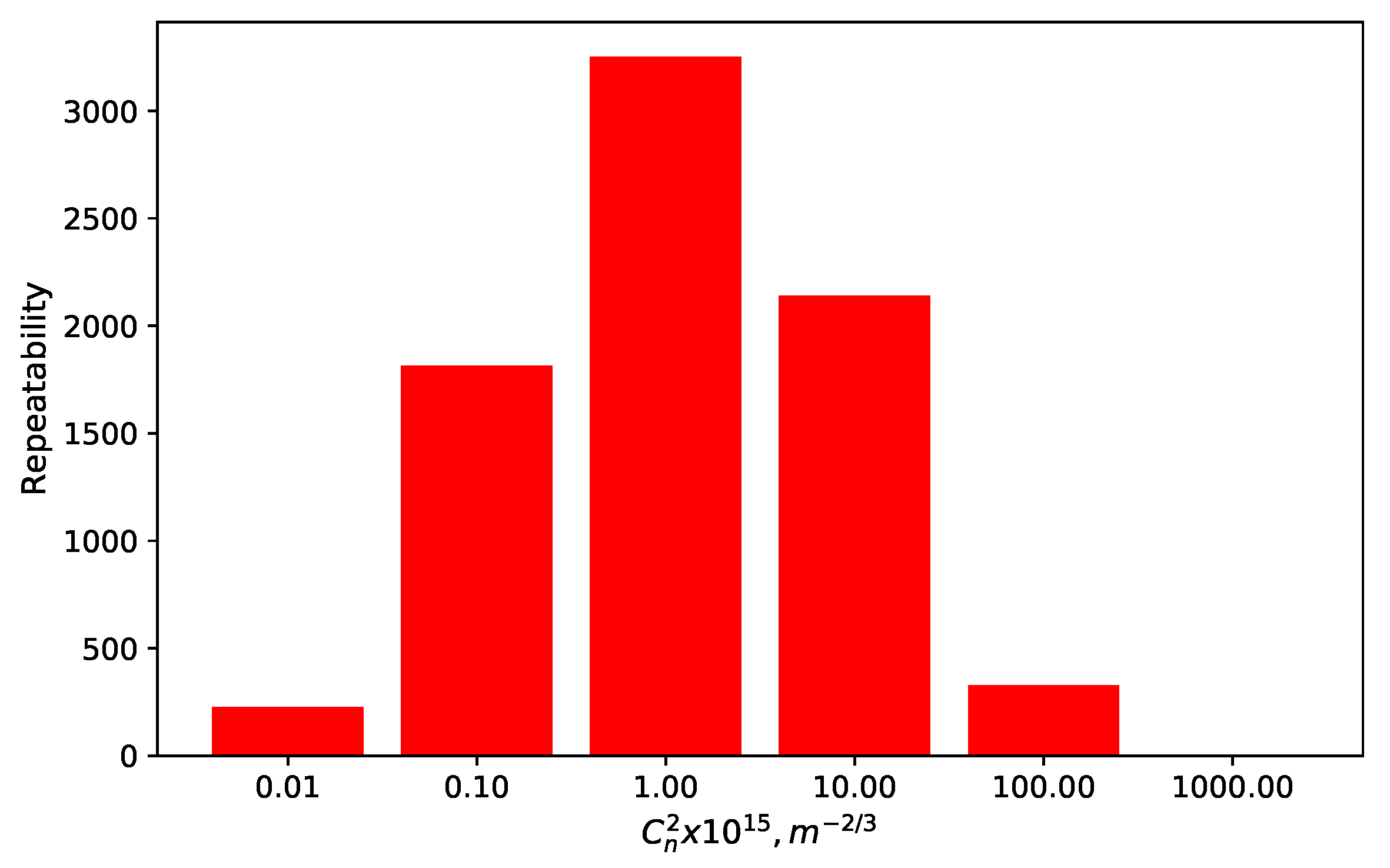
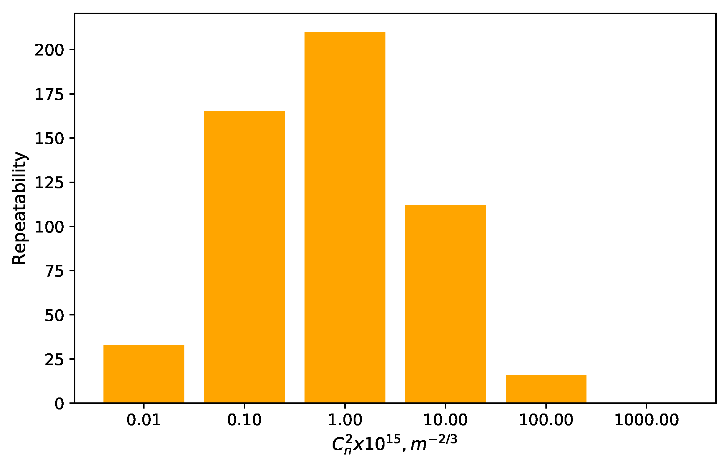
To analyze the temporal variability of the optical turbulence, we estimated the distributions of the repeatability of the structure characteristic of the air refractive index fluctuations in different seasons. The repeatabilities of the optical turbulence at the Baykal astrophysical observatory site in summer, autumn, winter, and spring are shown in Figure 3, Figure 4, Figure 5 and Figure 6, respectively.

Unfortunately, the measurement data include not only calm weather, clear sky, but also strong winds, cases when the wind speed exceeded 15 m/s. Quantitative estimates of the repeatability of the optical turbulence are shown in

Table 1. The repeatability R of the optical turbulence at the Baykal astrophysical observatory site in different seasons.

${\mathit{C}}_{\mathit{n}}^2$	R	${\mathit{C}}_{\mathit{n}}^2$	R
Summer		Spring
$\le {10}^{-17}{m}^{-2/3}$	0.03	$\le {10}^{-17}{m}^{-2/3}$	0.06
${10}^{-17}$–${10}^{-16}{m}^{-2/3}$	0.23	${10}^{-17}$–${10}^{-16}{m}^{-2/3}$	0.31
${10}^{-16}$–${10}^{-15}{m}^{-2/3}$	0.42	${10}^{-16}$–${10}^{-15}{m}^{-2/3}$	0.39
${10}^{-15}$–${10}^{-14}{m}^{-2/3}$	0.28	${10}^{-15}$–${10}^{-14}{m}^{-2/3}$	0.21
${10}^{-14}$–${10}^{-13}{m}^{-2/3}$	0.04	${10}^{-14}$–${10}^{-13}{m}^{-2/3}$	0.03
${10}^{-13}$–${10}^{-12}{m}^{-2/3}$	0	${10}^{-13}$–${10}^{-12}{m}^{-2/3}$	0
Autumn		Winter
$\le {10}^{-17}{m}^{-2/3}$	0.04	$\le {10}^{-14}{m}^{-2/3}$	0.02
${10}^{-17}$–${10}^{-16}{m}^{-2/3}$	0.17	${10}^{-14}$–$5\times {10}^{-14}{m}^{-2/3}$	0.1
${10}^{-16}$–${10}^{-15}{m}^{-2/3}$	0.37	$5\times {10}^{-14}$–${10}^{-13}{m}^{-2/3}$	0.33
${10}^{-15}$–${10}^{-14}{m}^{-2/3}$	0.36	${10}^{-13}$–$3\times {10}^{-13}{m}^{-2/3}$	0.4
${10}^{-14}$–${10}^{-13}{m}^{-2/3}$	0.05	$3\times {10}^{-13}{m}^{-2/3}$–$5\times {10}^{-13}{m}^{-2/3}$	0.13
${10}^{-13}$–${10}^{-12}{m}^{-2/3}$	0.01	$5\times {10}^{-13}$–${10}^{-12}{m}^{-2/3}$	0.02

. For convenience, repeatability is given in fractions R:

$$R=\frac{n_i}{N},$$

(5)

where $n_i$ is the number of cases in fixed range of $C_n^2$ changes, and N is the total number of cases in season. The analysis of obtained distributions shows that the structure of the optical turbulence changes significantly during the year. The strongest optical turbulence is observed in the winter, the mean value of $C_n^2=3.3\times {10}^{-13}{m}^{-2/3}$. The most favorable conditions are noted in summer, the mean value of $C_n^2=3.1\times {10}^{-15}{m}^{-2/3}$. It is significant that cases with weak turbulence (∼${10}^{-17}{m}^{-2/3}$) are observed throughout the year except for winter. In winter, the range of variations of $C_n^2$ is significantly narrowed. This may be due to the fact that the measurements covered the cold period with open water (the lake has not frozen yet). In addition, compared with spring and summer, the number of cases with moderate turbulence increases in the autumn.

Investigating the $C_n^2$ distributions discussed above, the surface layer turbulence is found to be weaker in summer than in winter. First of all, this is due to the suppression of the surface layer turbulence under the influence of the cold air over the lake in the summer. The high stability of the surface layer in the summer causes a decreasing of the turbulent fluctuations of both wind speed and air temperature. Moreover, significantly increasing the intensity of turbulence and a narrow range of $C_n^2$ changes in winter can be associated with the action of open (unfrozen) water. A warm water surface provides high vertical air temperature gradients inducing the development of convective instability.

3. The First Study of the Vertical Structure of the Surface Layer at the Baykal Astrophysical Observatory

In the previous chapter, we discussed the distributions of the repeatabilities of the structure characteristic of the air refractive index fluctuations that characterize the strength of the optical turbulence at height of 30 m. Although the optical turbulence is the most intense in the lower atmospheric layers, the upper layers can make a significant contribution to variations of Fried radius and the isoplanatic angle. There are a number of techniques for the measurements of the vertical profiles of atmospheric turbulence [12,13,14]. To recover the vertical profiles of the atmospheric turbulence, one may use methods based on the slope detection and the ranging (Slodar) technique. It should be noted that the vertical profiles of the optical turbulence may be restored with a Slodar technique with very high resolution (10 m or less) only in the lower layers of the atmosphere.

To determine the features of the vertical structure of the surface layer at the Baykal astrophysical observatory, we performed measurements of the wavefront local slopes using a Shack–Hartmann sensor of the large solar vacuum telescope for the time period from 26 June 2018 to 28 June 2018. Main parameters of the large solar vacuum telescope and the Shack–Hartmann wavefront sensor used are given in

Table 2. Main parameters of the large solar vacuum telescope and Shack–Hartmann wavefront sensor.

Parameter	Value
Aperture diameter	600 mm
Focal length	40 m
Radiation wavelength	0.535 $\mathsf{\mu }$m
Camera resolution	640 × 480 $pix$
Pixel size	7.4 $\mathsf{\mu }$m
Number of subapertures	8 × 8
Equivalent size of subaperture	7.5 cm
Angular pixel size	0.83 ${}^{″}$
Frame frequency	70 Hz
Exposure	30 ms

.

Motion of images in each subaperture is estimated using extended light sources—images of solar edge. According to formula [14], we estimated cross-correlation functions:

$$C_s(i,j)=\langle \delta x_1·\delta x_2\rangle ,$$

(6)

where

$$\delta x_1(i,0)=\sum _{i=m}^t{s}_m\left(i\right)-s_m\left(0\right),$$

(7)

$$\delta x_2(i,\beta )=\sum _{i=1}^m{s}_m(i+\beta z_m)-s_m\left(\beta z_m\right).$$

(8)

Indices 1 and 2 correspond to light sources (the individual spaced regions of the solar edge), $z_m$ is the height of the turbulent layer m, $s_m\left(0\right)$ is wavefront slope induced by the turbulent layer m on reference subaperture, $i,j$—indices of the subapertures, and $\beta$—angle between "axial" and "non axial" objects within the field of view of the given subaperture.

In calculations, there is a task to extract the local slopes of the wavefront measured by the Shack–Hartmann sensor using the solar edge images. Multiple centroiding techniques are applied to extract the local slopes including analysis of gravity centers, weighted gravity centers, filtering, and correlation based centroiding techniques. To extract the local slopes of the wavefront, we used a weighted gravity centers technique [15].

Applying the standard technique [13], we estimated the functions $C_s$ which characterize the vertical profiles of the optical turbulence in the lower layers. The technique is based on a relation between the wavefronts’ distortions spaced at the telescope pupil and altitude of the turbulent layer through which the wavefronts of a few light sources pass. Positive correlation coefficients of wavefront distortions indicate the existence of a turbulent layer. The examples of calculated functions $C_s$ to determine the vertical structure of the atmospheric turbulence are shown in Figure 7.

Analysis of the calculated functions depicted in Figure 7 shows that there are a few peaks. These peaks are induced by the individual turbulent layers. The height of the turbulent layer is determined by angle between the spaced fragments of the solar edge according to formula [14]:

$$z_m=\frac{D}{n\theta }cos\alpha .$$

(9)

$\alpha$ is the zenith angle, $D/n$ is the distance between centers of analyzed subapertures, and $\theta$ is the angle between individual spaced regions of the solar edge. The peaks correspond the angles of 5–10 and 27–35 arcsec. By triangulating the wavefront distortions and using formula (9), we estimate that the heights corresponding to $\theta$ are 1500–3000 m and 400–600 m, respectively.

4. Conclusions

The research results show that atmospheric turbulence in the surface layer at the Baykal astrophysical observatory site is most developed in the winter. At this time, the number of cases with weak turbulence is minimal. The best conditions for astronomical experiments are observed in the summer. Atmospheric turbulence is suppressed in summer. It was found that in the autumn period the distribution shape is violated: there is mainly moderate turbulence. Increased repeatability of moderate and even weak turbulence is noted in the spring. The nature of the changes of the optical turbulence is consistent with astronomical observations qualitatively. Calculations have enabled quantitative estimates of changes of the optical turbulence. Furthermore, we plan to use an improved algorithm [4] to calculate the statistics of turbulent characteristics. Increased accuracy is ensured by taking into account the shape of the turbulence spectrum at low frequencies.This will allow a detailed study of the structure of atmospheric flows and energy exchange between large and small scales in rough terrain.

In addition, we performed the measurements of the local slopes of the wavefront. By triangulation of local slopes, we reveal the heights of the turbulent layers in the atmospheric boundary layer at the Baykal astrophysical observatory site. The obtained heights (1500–3000 m and 400–600 m) are consistent with the data of lidar observations [16].

The obtained estimations of the structure characteristic of the air refractive index fluctuations as well as revealed features in the vertical distribution of the turbulence will be used for development of the spectral model of turbulent atmosphere [1,17].