Forecasting Particulate Matter Concentration Using Linear and Non-Linear Approaches for Air Quality Decision Support

Abstract

Air quality status on the East Coast of Peninsular Malaysia is dominated by Particulate Matter (PM₁₀) throughout the years. Studies have affirmed that PM₁₀ influence human health and the environment. Therefore, precise forecasting algorithms are urgently needed to determine the PM₁₀ status for mitigation plan and early warning purposes. This study investigates the forecasting performance of a linear (Multiple Linear Regression) and two non-linear models (Multi-Layer Perceptron and Radial Basis Function) utilizing meteorological and gaseous pollutants variables as input parameters from the year 2000–2014 at four sites with different surrounding activities of urban, sub-urban and rural areas. Non-linear model (Radial Basis Function) outperforms the linear model with the error reduced by 78.9% (urban), 32.1% (sub-urban) and 39.8% (rural). Association between PM₁₀ and its contributing factors are complex and non-linear in nature, best captured by an Artificial Neural Network, which generates more accurate PM₁₀ compared to the linear model. The results are robust enough for precise next day forecasting of PM₁₀ concentration on the East Coast of Peninsular Malaysia.

1. Introduction

Air quality in a developing country such as Malaysia has decreased gradually because of rapid urbanization, industrialization and population growth [1]. Southeast Asia cities, including Malaysia are notified as surrounded by particulate matter (PM₁₀) in air quality problems [2,3,4,5]. PM₁₀ or known as coarse particle is defined as the particulate matter that having an aerodynamic diameter of less than (≤) 10 µm [6]. PM₁₀ had received special attention especially in Peninsular Malaysia, as it was proven to have the highest index through the Air Pollutant Index (API) compared to other criteria pollutants annually. Moreover, the status of API in the East Coast of Peninsular Malaysia was noted as having a good to moderate level, where only a few days were recorded to have unhealthy levels of PM₁₀ concentration during the dry season months (May to September) [3]. The main sources of PM₁₀ in Malaysia are emissions from the motor vehicles, heat and power plants, industries and open combustion. High concentrations of PM in the atmosphere (for instance African dust) happen when there exists a low amount of rainfall combined with high temperatures, which prompts the re-suspension of dust. Arid areas such as the Sahara contribute to natural mineral dust. Anthropogenic activities associated with various gaseous and particulate emissions can be determined by air quality temporal and spatial variations in a region. Engine combustion (diesel and petrol), industrial, mining, building, cement, agriculture and many more are examples of an anthropogenic source of particulate matter emission. Motor vehicle emission occurs mostly in urban areas where population densities are much higher than the global average. PM₁₀ is under escalated toxicological and epidemiological examinations [7] and has been considered in affecting human health [8], namely by causing diseases such as respiratory illness [9] and cardiovascular diseases [10]. World Health Organization (WHO) additionally utilized PM₁₀ as a marker of air contamination introduction as it is noteworthy as an environmental hazard component worldwide [11]. Considering the proven adverse health effects especially on human health, the forecasting of PM₁₀ in advance and the assessment of the model is important, as it allows authorities to take control measures to ensure the health of the population and improve air quality in specific locations.

The problem of atmospheric pollutants such as PM₁₀ concentration is not a straightforward issue of controlling the emission sources. The complexity of PM₁₀ concentration in the atmosphere relies on meteorological factors and gaseous pollutants [12] with multi-confronted qualities over different spatial-transient scales. The meteorological factors and gaseous pollutants are ambient temperatures, relative humidity, wind speed, wind direction, global radiation, rainfall amount, mean sea level pressure (MSLP), sulphur dioxide (SO₂), carbon monoxide (CO) and nitrogen dioxide (NO₂). Meteorological factors have a strong influence on ambient air quality through the various mechanisms in the atmosphere, both directly and indirectly. Wind speed and wind direction are responsible for some mechanisms of particle emission in the atmosphere, such as re-suspension of particles and diffusion, as well as the dispersion of particles. The increase of wind speed results in low pollutant concentration, as it dilutes the pollutant. Rain removes particulates in the atmosphere through a “scavenging” process, and it is able to dissolve other gaseous pollutants. The frequent high rainfall amount generally results in better air quality. Precipitation provides the information on the removing process of pollutants in the atmosphere through wet deposition. PM₁₀ can be scavenged from the atmosphere by rain through two basic processes. The first is termed in-cloud scavenging by the cloud elements and precipitation, usually called rainout or snow out. It is the result of the aerosol serving as a cloud nucleus or undergoing capture by cloud cover water or ice particles. The second process is termed below-cloud scavenging, usually called washout. This is a result of the removal of the sub-cloud aerosol by the raindrops as they fall. Measuring ambient temperature strengthens air quality assessment, air quality modeling and anticipated forecasting model. Recorded daily maximum temperatures are linked with low wind speed, little precipitation and high daily maximum mixing height. The temperature typically increases evaporation processes and the high relative humidity will induce the increment of the amount of water vapor and rain that will remove the pollutants in the atmosphere. MSLP and PM₁₀ concentrations have a positive relationship. At the point where the ground is controlled by a low MSLP, high MSLP air mass is counter-clockwise around the focal point of the flow. Accordingly, an updraft is created in the focal point and the amount of wind increases, which helps pollutants moving upwards. At that point, PM₁₀ concentrations are getting modest. Conversely, as the high MSLP dominates the ground, the air at the center part is reduced and demonstrates a clockwise rotation. At that point, the weather is decent and wind speed shows an increment. Therefore, this condition is suitable for the buildup of a thermal inversion layer. The thermal inversion layer will prompt a stable atmospheric condition. In this way, pollutants are substantially harder to dilute and can be found on the surrounding land surface. Subsequently, under a control of stable condition, air pollution will increase. PM₁₀, after it is emitted to the atmosphere, is subjected to several meteorological factors and gaseous pollutants [13]. These factors control the arrangement, transportation and expulsion of particulates in the atmosphere, which gets distinctly complex and shows a non-linear character [14]. Throughout the years, various factual methodologies, such as physically-based deterministic and statistical approaches, have been proposed to forecast the PM₁₀ concentration [15,16,17,18]. In spite of their obvious valuable contributions, no earlier conclusion can be drawn regarding the appropriate model without considering distinctive meteorological factors and gaseous pollutants. Understanding the interaction between these factors and PM₁₀ concentration is useful in forecasting strategies in Malaysia.

The relationship between PM₁₀ concentration, meteorological factors and gaseous pollutants has been proven statistically by using several multivariate analyses, especially the development of Multiple Linear Regression (MLR) models to forecast PM₁₀ concentration [19,20,21]. Unfortunately, MLR relies on several assumptions, such as that the independent variables are linearly independent (multi-collinearity), that there is homogeneity of variance (homoscedasticity) and that the variables are normally distributed [22,23,24]. However, in a real world situation, the PM₁₀ concentration data that is measured in terms of temporal variation does not demonstrate linear characteristics, and therefore, are hard to examine and forecast accurately. The development of traditional modeling techniques such as MLR in nonlinear situation is proven to give less accuracy in forecasting [25]. Thus, for the purpose of exploration of real data PM₁₀ concentration temporal data, it seems crucial that non-linear models; for instance, Artificial Neural Networks (ANN) were developed for more accurate and precise PM₁₀ concentration forecasting [26]. Furthermore, ANN quickly processes the information with no particular presumptions of the way of the non-linearity [27]. Therefore, the development of ANN models in forecasting PM₁₀ concentration is important as ANN models can capture the complexity and non-linear character of PM₁₀ in the atmosphere under the influence of meteorological and gaseous pollutants.

Undeniably, various studies have been performed on PM₁₀ forecasting, worldwide and in Malaysia. However, this effort has less been reported especially in the eastern part of Peninsular Malaysia, rather than the western part of Peninsular Malaysia. The increment of year by year of industrialization, urbanization and population on the East Coast of Peninsular Malaysia is believed to reduce the air quality and affect human health [28]. Hence, it is advantageous to develop three forecasting algorithm techniques, which comprise linear and non-linear algorithms. In the real world situation, an area is distinctly differentiated through land use type, and therefore, different land use that is known as the majority notified in the East Coast of Peninsular Malaysia composed of the urban, suburban and rural areas which representing the cities of Kuala Terengganu and Kota Bharu, Kuantan, and Jerantut, respectively, were selected as the field of interest. Moreover, no comprehensive modeling study has been undertaken that attempts to research the variation of PM₁₀ concentration caused by different meteorological factors and gaseous pollutants in the East Coast of Peninsular Malaysia. The combination of this knowledge is important in building significant PM₁₀ forecasting tools for beneficial information in air quality management. In this study, the predictive ability of the linear model, for instance the Multiple Linear Regression (MLR), and that of non-linear models approaches, such as the Multi-Layer Perceptron (MLP) and Radial Basis Function (RBF), for PM₁₀ concentration forecasting were investigated at the study areas. These models were critically assessed through performance indicators keeping in mind the end goal to choose the best-fitted model for each study areas for accurate forecasting.

2. Materials and Methods

2.1. Study Area

This research was performed in the East Coast of Peninsular Malaysia, which covers the states of Pahang, Terengganu and Kelantan. Two urban sites were selected in this research, located at Kuala Terengganu, Terengganu and Kota Bharu, Kelantan. One sub-urban site was located at Kuantan, Pahang and one rural site was located at Jerantut, Pahang. Two urban areas were selected in this study due to their future rapid development as planned by the Malaysian government through the National Physical Plan, more specifically the East Coast Economic Region (ECER). Moreover, construction of the East Coast Rail Line (ECRL) will transform several areas to urban areas. Furthermore, the complexity of urban areas is another reason for the selection of two urban areas for better validating and testing the robustness of models being developed. The study areas are depicted in Figure 1. The details information in terms of station ID, the location of the air quality monitoring station, the classification or land use, as well as longitude and latitude of each selected air quality monitoring stations, is stated in

Table 1. Selected air quality monitoring stations in East Coast of Peninsular Malaysia.

Site	Station ID	Location	Classification	Latitude, Longitude
S1	CA0034	Chabang Tiga Primary School, Kuala Terengganu	Urban	5°18.455′ N 103°07.213′ E
S2	CA0022	Tanjong Chat Secondary School, Kota Bharu, Kelantan	Urban	6°08.443′ N 102°14.955′ E
S3	CA0014	Indera Mahkota Primary School, Kuantan, Pahang	Sub-Urban	3°49.138′ N 103° 17.817′ E
S4	CA0007	Batu Embun Meteorological Station, Jerantut, Pahang	Rural	3°58.238′ N 102°20.863′ E

.

2.2. Data Acquisition

The secondary data has a 15-year time span, from 1 January 2000 to 31 December 2014. This long term historical data was needed, as it can represent the variation of pollutants comprehensively [29]. The PM₁₀ data used in this research was recorded as a major aspect of a Malaysian Continuous Air Quality Monitoring (CAQM) program, using the β-ray attenuation mass monitor (BAM-1020), as made by Met One Instruments Inc. The instrument basically is built-in with a cyclone and PM₁₀ head particle trap, fiberglass tape, flow control and a data logger. This instrument delivers a fairly high resolution of 0.1 µg/m³ at a 16.7 L/min flow rate, with lower detection limits of 4.8 µg/m³ and 1.0 µg/m³ for 1h and 24 h, respectively [30]. The installation, operation and maintenance of Air Quality Monitoring Stations (AQMS) are performed by Alam Sekitar Malaysia Sdn. Bhd (ASMA) on behalf of the Malaysian Department of Environment [31].

The forecasting of PM₁₀ concentration in this study is on a daily basis [32]. In order to gain a better understanding of PM₁₀ concentration, 10 daily averaged parameters were taken into consideration. This study used a daily average of particulate matter with an aerodynamic diameter less than 10 µm (PM₁₀, µg m⁻³), ambient temperature (AT, °C), relative humidity (RH, %), wind speed (WS, m s⁻¹), global radiation (GR, MJ m⁻²), Mean Sea Level Pressure (MSLP, hPa), rainfall amount (RA, millimeter), carbon monoxide (CO, ppm), nitrogen dioxide (NO₂, ppm) and sulphur dioxide (SO₂, ppm). The data were acquired from the Air Quality Division, Department of Environment (DOE), Ministry of Natural Resources and Environment of Malaysia, as well as from the Malaysian Meteorological Department (MMD), Ministry of Energy, Science, Technology, Environment and Climate Change. The reliability of data from DOE has consistently assured through quality assurance and quality control [33]. Moreover, the procedures used to follow the standard drawn by United States of Environmental Protection Agency (USEPA) [30].

The data were divided into two sets; 70% (N = 3835) for the development of the linear model (Multiple Linear Regression (MLR)). In the case of non-linear models, the Multi-Layer Perceptron (MLP) and the Radial Basis Function (RBF) were used, and the remaining 30% (N = 1644) for model validation [34,35]. The separation of this data is important in ANN as a method of early stopping. This early stopping technique is important, as it avoids any underfitting and overfitting of an ANN network [36] and allows the network to stop training the model itself when the verification errors starts to increase when compared to the training error. The lowest squared error on the verification is supposed to have the best generalization ability [37]. During the training of ANN models, the stopping criteria are the number of epochs and the decrease in the training error [38]. The model validation for the linear model, in the case for non-linear models, known as model testing, is aimed at measuring the agreement of the models, generalizing with an independent data set [39].

2.3. Imputation of Missing Values

Data in the dataset might missing due to the instruments problem, weather, maintenance and changing of siting monitor. This can introduce errors while developing the prediction model. Missing data in terms of percentage (%) were calculated by dividing the numbers of missing data and numbers of total data; then, data were multiplied with 100%. Linear interpolation technique was applied in the imputation of missing values, as the missing percentage was less than 25%. Linear interpolation imputed the missing values using the mean value of the last and first available data in the dataset in SPSS^® version 23 [40]. The formulation is given as:

$$f\left(x\right)=f\left(x_0\right)+\frac{f\left(x_1\right)-f\left(x_0\right)}{x_1-x_0}\times \left(x-x_0\right)$$

(1)

where $x$ = independent value, $x_1$ and $x_0$ = known values of the independent variable and $f\left(x\right)$ = value of dependent variable for a value of the independent variable.

2.4. Data Normalization

Units of measurement for the variables are different; thus, data normalization is needed. Min-max technique of data normalization is adapted in this study which in the end, the values are between 0 and 1 [0, 1] [41,42] for an accurate predictive model [43]. The technique is based on the following [44]:

$$z_i=\frac{x_i-min\left(x\right)}{max\left(x\right)-min\left(x\right)}$$

(2)

where $x=\left(x_1,\dots , x_n\right)$ and $z_i$ is the $i\mathrm{th}$ normalized data.

2.5. Multiple Linear Regression (MLR)

The regression analysis is most frequently used for forecasting. The objective is to build up a mathematical model that can be utilized to forecast the dependent variable based on the inputs of independent variables [45,46]. The coefficient of determination (R²) is a marker to decide if the information gives adequate proof to show that the general models contribute to the overall variance in data. In the MLR model, the error term signified by ε is thought to be regularly disseminated with the mean 0 and change σ² (which is constant). Similarly, $\epsilon$ is thought to be uncorrelated. In this research, it was accepted that the MLR model has $k$ independent variables and that there are $n$ observations. In this way, the regression model can be composed as [47]:

$$Y_i={\beta }_o+{\beta }_1{x}_{1i}+\cdots +{\beta }_k{x}_{ki}+{\epsilon }_i \mathrm{with}i=1,\dots ,n$$

(3)

where $b_i$ is the regression coefficients, $x_i$ is independent variables and $\epsilon$ is a stochastic error associated with the regression.

Collinearity occurs when two model covariates have a linear relationship. This makes the individual contribution of each variable difficult to discern, introduces redundancy and makes the model excessively sensitive to the data. The multi-collinearity assumption was verified by Variance of Inflation Factor (VIF) accompanied with the regression output, where as long as the VIF is under 10 the conducted regression should be fine, where there is no multi-collinearity between the independent variables [24]. The VIF is given by:

$$VI{F}_I=\frac{1}{1-R_i^2}$$

(4)

where $VI{F}_i$ is the variance inflation factor related with the $i\mathrm{th}$ predictor and $R_i^2$ is the multiple coefficients of determination in a regression of the $i\mathrm{th}$ predictor on all other predictors.

By performing the Durbin-Watson (D-W) Test, autocorrelation can be recognized. Autocorrelation basically uncovers the capability of PM₁₀ concentration of current day to estimate the following day of PM₁₀ concentration. The test values can change in the vicinity of 0 and 4 with an estimation of 2 implying that the lingering is uncorrelated [19]. The D-W is given by:

$$D-W=\frac{{\sum }_{i=1}^n{\left(e_i-e_{i-1}\right)}^2}{{\sum }_{i=1}^n{e}_i^2}$$

(5)

where $n$ is number of data and $e_i$ = $y_i-{\overline{y}}_i$ ($y_i$ = observed data and ${\overline{y}}_i$ is the forecasted data).

2.6. Multi-Layer Perceptron

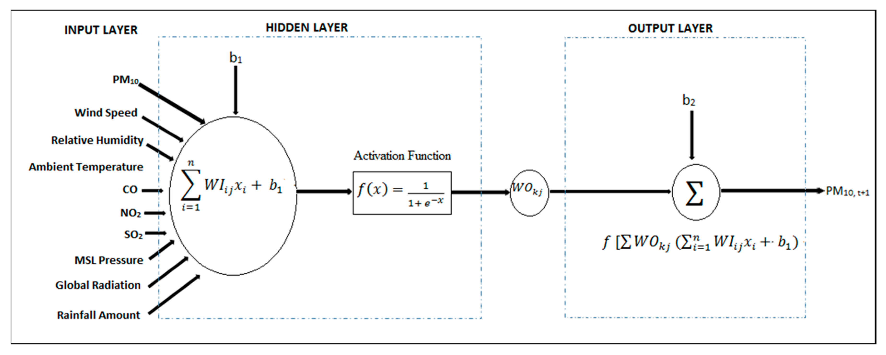
MLP models consist of several types, but the most commonly used in air pollution forecasting is the Feed Forward topologies of Multi-Layer Perceptron (MLP) as shown in Figure 2 [37,48,49].

The MLP starts when the interested input parameters are fed into the network. These input parameters provide input signals and these signals are sent to the network starting from the input layer to the hidden layer and from the hidden layer to the output layer. The scaled input vector, which introduces neurons to the input layer, is multiplied by weights, which is a real number quantity. The neuron in the hidden layer sums up this information, including bias.

$$y_o={\sum }_{i=1}^n{w}_i{x}_i+b$$

(6)

This weighted sum information is still in its linear model. The non-linearity of information or model occurs when it is passing through the activation or transfer function.

$$f\left(x\right)=\frac{1}{1+e^{-x}}$$

(7)

Then:

$$y_o=f \left[{\sum }_{i=1}^n w_i{x}_i+b\right]$$

(8)

where $y_o$ is the output, $W_i$ is weight vector, $X_i$ is the scaled input vector, $b$ is the bias, $f$ is the transfer function and $x$ represents the total sum of weighted inputs.

Once the error signal is computed, the process of model fitting ends. The difference between target and output is used to compute the error signal in the model, which corresponds to the input [50]. Mathematically, the equation of MLP with several numbers of neurons is given as:

$$y_o=f [\sum W{O}_{kj} ({\sum }_{i=1}^n W{I}_{ij}{x}_i+b_1)+b_2]$$

(9)

where $W{I}_{ij}$ and $W{O}_{kj}$ are the weights of input and output layers, respectively, and $b_1$ and $b_2$ are biased in the input and output layer, respectively. The determination of various neurons in the hidden layer is an exceptionally basic assessment and is known to be user-specified [51]. Furthermore, the excessive number of neurons in the hidden layer may bring about underfitting or overfitting, which builds the noteworthy blunders of the created models [34]. This situation may happen amid the training stage. The number of neurons in the hidden layer is found by the trial and error approach, which starts with one neuron and progressively includes more neurons one by one [36,52]. Keeping in mind the end goal to decide the optimum number of neurons in the hidden layer in the most targeted way, this trial and error method was rehashed 10 times at arbitrarily appointed picked data points [43], and the optimum number of neurons was selected in view of the least performance error (average of all trials) as measured by Root Mean Square Error (RMSE) [41,52] and R² values [52].

There are no standard rules on the minimum and maximum number of neurons in the hidden layer [53]; however, the scope of an optimum number of neurons in the hidden layer has been recommended by a few researchers. The proper number of neurons in hidden layer ranges from $2 \sqrt{M}+N$ to $2M+1$; $M$ is the number of input and $N$ is the number of output node [54]. The diverse number of neurons were tried in MLP models by utilizing $\frac{M}{2}-2$ up to $\frac{M}{2}+2$, where $M$ is the number of input variables [55]. It was recommended that the number of neurons in the hidden layer as $M+1$ [56], and $\left(\frac{2}{3}\right)\times \left(M+N\right)$ [57]. Other than that, a previous study proposed and effectively demonstrated that the number of neurons in the hidden layer is not bigger than twice the number of inputs [58].

The activation or transfer function played an important role in ANN by producing a non-linear decision through non-linear blends of weighted inputs. This activation function then transforms input signals into output signals. This activation function presents the non-linearity in the MLP model, and subsequently contrasts it from the linear model. Sigmoid units of activation functions map the input to a value in the range of 0 to 1. This research utilizes three sigmoid functions that are generally utilized as a part of MLP; for example, purelin (linear), log-sigmoid (logsig) and hyperbolic tangent sigmoid (tansig) [34,52]. The tansig transfer function in the hidden layer is recommended to be utilized by previous studies [55,59], while the logsig transfer function is proposed by [43,60] and a linear (purelin) activation function is used in the output layer [55].

In order to train the optimum configuration of the MLP network, the learning rate was set to 0.05 [59]. This prevents the network from diverging from the target output; additionally, it enhances the general execution. The bias is defined as 1 [34], both at the hidden layer and output layer for the activation function (sigmoid) employment. The initialization of the MLP network was trained with 5000 epochs [37]. Therefore, considering the above-stated topology and criteria of MLP, several networks consisting three-layered MLP were trained in order to optimize or to find the best activation function of hidden and output layer, as well as the number of nodes or neurons in the hidden layer. The development of MLP is generally composed of three main steps: (1) define the training sets; (2) train the MLP; (3) apply the network to a new set of data (Testing). All implementations and computations were performed using Matrix Laboratory (MATLAB) (MathWorks, Inc. Massachusetts USA) [61].

2.7. Radial Basis Function

MLP networks inherent several drawbacks which include slow convergence speed, network topology specification and poor generalization performance [62]. Although several of its optimization techniques can be employed on the network, most will result in computationally high demands, and therefore, it is difficult to put this MLP model into practice. The RBF network was developed, which visualizes a more effective algorithm for a faster convergence speed and good generalization ability [63]. The architecture of RBF model is shown in Figure 3.

RBF consists of three layers; input layer, hidden layer and output layer. In terms of training time, RBF has a shorter training time as compared with other models [64]. Its specialty is that the hidden layer is composed of a transfer function known as Gaussian (radial basis). These hidden neurons work in measuring the weight distance between the input layer and output layer [65]. Two RBF parameters, known as center and spread, are important as the first weight connecting the input layer and hidden layer. The second weight connects the radial basis function to the output layer. The Gaussian is given as [66]:

$$øj\left(x\right)=\exp (-\frac{{\Vert x-\mu j\Vert }^2}{2{\sigma }^{2}j}),$$

(10)

where $x$ represents the input, $\mu$ the center of the RBF unit and ${\sigma }_j$ is the spread of the Gaussian basis function.

The optimum number of nodes in hidden layer depends on the behavior of training dataset. The training process concludes the optimum number of nodes in the hidden layer. A different spread number is used in this study [36] and the number of nodes is equivalent to the number of epochs in for the trained model. Training error is constant at 0.001 [62], while the suitable spread is determined through a trial and error method [42], with a scale of 0.1 from 0 to 1 [67]. The performance is based on the lowest RMSE and highest R² values for the best predictive model. The output layer is the linear function for executable results. The output layer is given with [68]:

$$y_{k\left(x\right)}={\sum }_{j=1}^M W_{kj}{\varphi }_j\left(X\right)+W_{ko}$$

(11)

where $M$ = number of basis functions, $x$ = output data vector, $W_{kj}$ = weighted connection between the basis function and output layer, ${\varphi }_j$ = nonlinear function of unit $j$ in the RBF and $W_{ko}$ = weighted connection in the output layer.

2.8. Performance Indicators

The selection of the best-fitted model, MLR, MLP or RBF at each site, was based on the performance indexes or performance indicators. Performance Indicator (PI) measures two things: (1) accuracy measure and (2) error measure. The accuracy measures evaluate values from 0 to 1, whereby the best model is considered when the evaluated values are close to 1, while the best model for error measures are selected if the evaluated value is close to 0 [69,70].

Performance indicators that were used are [29,69]:

(a)

Root Mean Square Error (RMSE):

$$RMSE={[(\frac{1}{n-1}){\sum }_{i=1}^n {\left(P_i-O_i\right)}^2]}^{1/2}$$

(12)

(b)

Index of Agreement (IA):

$$IA=\left[\frac{{\sum }_{i=1}^n{\left(P-O_i\right)}^2}{{\sum }_{i=1}^n (|P_i-\overline{O}|+{|O_i-\overline{O}|}^2}\right]$$

(13)

(c)

Normalized Absolute Error (NAE):

$$NAE=\frac{{\sum }_{i=1}^n |P_i-O_i|}{{\sum }_{i=1}^n O_i}$$

(14)

(d)

Correlation Coefficient (R²):

$$R^2={\left(\frac{{\sum }_{i=1}^n\left(P_i-\overline{P}\right)\left(O_i-\overline{O}\right)}{n·S_{pred }·S_{obs}}\right)}^2$$

(15)

(e)

Prediction Accuracy (PA):

$$PA={\sum }_{i=1}^n\frac{\left(P_i-\overline{P}\right)\left(O_i-\overline{O}\right)}{\left(n-1\right)S_{pred}{S}_{obs}}$$

(16)

where $n$ = total number measurements at a particular site, $P_i$ = forecasted values, $O_i$= observed values, $\overline{P}$ = mean of forecasted values, $\overline{O}$ = mean of observed values, S_pred = standard deviation of forecasted values and S_obs = standard deviation of the observed values.

3. Results and Discussion

3.1. Descriptive Statistics

The descriptive statistics and boxplot showing the temporal variation of PM₁₀ concentrations during the study period (2000–2014) for each site are summarized in

Table 2. Descriptive statistics (mean ± standard deviation) of air pollutants and meteorological parameters. PM₁₀: Particulate Matter; CO: Carbon Monoxide; SO₂: Sulphur Dioxide; NO₂: Nitrogen Dioxide.

Site	S1	S2	S3	S4
PM10 (µg/m3)	51.72 ± 15.09	40.74 ± 14.32	34.08 ± 12.12	37.34 ± 14.79
Wind Speed (m/s)	1.50 ± 0.42	1.49 ± 0.47	1.81 ± 0.45	1.01 ± 0.19
Temperature (°C)	27.33 ± 1.45	27.00 ± 1.38	26.94 ± 1.51	26.45 ± 1.54
Relative Humidity (%)	81.14 ± 5.33	79.36 ± 5.68	83.94 ± 6.69	82.83 ± 5.16
Rainfall Amount (mm)	7.52 ± 21.23	7.48 ± 20.68	8.88 ± 23.72	5.93 ± 13.41
Atmospheric Pressure (hPa)	1010.18 ± 1.74	1010.01 ± 1.72	1009.86 ± 1.54	1009.97 ± 1.54
CO (ppm)	0.45 ± 0.15	0.65 ± 0.24	0.36 ± 0.14	0.30 ± 0.13
SO2 (ppm)	0.00093 ± 0.00075	0.00099 ± 0.0011	0.0013 ± 0.00076	0.00080 ± 0.00068
NO2 (ppm)	0.0055 ± 0.0016	0.0072 ± 0.0027	0.0059 ± 0.0020	0.0020 ± 0.00088
Solar Radiation (MJ/m2)	Not Available	18.37 ± 5.54	16.80 ± 4.86	Not Available

.

3.2. Multiple Linear Regression Model

The MLR models were developed and the models’ summary is depicted in

Table 3. Summary of the Multiple Linear Regression (MLR) models for PM₁₀ forecasting. VIF: Variance of Inflation Factor; D-W: Durbin-Watson. R²: Correlation Coefficient.

Site	Model	R2	Range of VIF	D-W Statistics
S1	PM10,t+1 concentration = 0.037 + 0.709(PM10) − 0.231(Rainfall Amount) + 0.044(MSLP) + 0.101(NO2) + 0.039(Wind Speed) − 0.023(SO2) − 0.027(CO)	0.594	1.077–1.921	2.007
S2	PM10,t+1 concentration = 0.116 + 0.763(PM10) − 0.148(Rainfall Amount) − 0.030(CO) + 0.034 (Ambient Temperature) − 0.040 (Relative Humidity) − 0.027(SO2)	0.601	1.116–1.513	2.021
S3	PM10,t+1 concentration = 0.016 + 0.805(PM10) + 0.020 (Global radiation) + 0.032(NO2)	0.680	1.054–1.205	2.131
S4	PM10,t+1 concentration = 0.044 + 0.820(PM10) − 0.086(Rainfall Amount) − 0.025(Wind Speed) − 0.009(SO2) − 0.024(CO) + 0.019(NO2)	0.706	1.012–1.926	2.150

. The range of the Variance Inflation Factor (VIF) for the independent variables of the MLR model was in the range of 1.012–1.926. The VIF values were lower than 10, which demonstrates that the multi-collinearity issue does not exists in the model. Durbin Watson (D-W) statistics demonstrate that the models are able to cater the autocorrelation, as the values were in the range of 2.007–2.150. The residual (error) is critical in choosing the ampleness of the factual model. On the off chance that the error demonstrates any sort of pattern, it is interpreted that the model does not deal with all of the methodical data (Figure 4 and Figure 5). Figure 4 indicates histograms of the residuals of PM₁₀ models. The residual analysis shows that the residuals were normally distributed with zero mean and constant variance. The plots of fitted values with residuals for the PM₁₀ model are shown in Figure 5, indicating that the residuals are uncorrelated because the residuals are contained in a horizontal band and hence obviously that variance is constant.

3.3. Multi-Layer Perceptron Model

The number of neurons in the hidden layer is assessed through a few references as expressed in Section 2.6 (Materials and Methods). The range of the tried number of neurons in the hidden layer is organized and appeared in

Table 4. Calculated range of neurons.

Site	Number of Inputs	Range of Neurons
1	9	1–19
2	10	1–21
3	10	1–21
4	9	1–19

.

The best combination of different sigmoid functions, which includes Logsig, Tansig and Purelin, were determined through several trials in the training phase. It should be noted that the best results are marked with bold (

Table 5. MLP models of different activation functions. RMSE: Root Mean Square Error. Best results marked in bold.

Activation Function for Hidden Layer	Activation Function for Output Layer	Optimum Number of Neurons in Hidden Layer	RMSE (µg/m3)	R2
(a) Site 1
Logsig	Purelin	18	8.49	0.691
Logsig	Tansig	17	8.58	0.684
Tansig	Purelin	17	8.54	0.687
Tansig	Logsig	18	8.57	0.685
Logsig	Logsig	17	8.60	0.683
Tansig	Tansig	19	8.51	0.690
(b) Site 2
Logsig	Purelin	20	9.44	0.722
Logsig	Tansig	21	9.45	0.720
Tansig	Purelin	21	9.48	0.718
Tansig	Logsig	20	9.49	0.716
Logsig	Logsig	19	9.50	0.715
Tansig	Tansig	20	9.45	0.720
(c) Site 3
Logsig	Purelin	19	7.60	0.766
Logsig	Tansig	21	7.63	0.761
Tansig	Purelin	17	7.59	0.767
Tansig	Logsig	21	7.62	0.761
Logsig	Logsig	17	7.64	0.760
Tansig	Tansig	20	7.60	0.765
(d) Site 4
Logsig	Purelin	18	9.57	0.794
Logsig	Tansig	15	9.59	0.792
Tansig	Purelin	19	9.59	0.792
Tansig	Logsig	19	9.65	0.786
Logsig	Logsig	18	9.61	0.790
Tansig	Tansig	17	9.62	0.790

). The selection of the best model during the training phase is strictly based on the R² and RMSE. Site 1, Site 2 and Site 4 have the best combination of Logsig-Purelin activation function while Site 3 has the best combination of Tansig-Purelin activation function. The combination of Logsig/Tansig-Purelin activation functions is similar to the results deliberated by [43,55,59,60] and has been proposed by several researchers in training the MLP model [34,52]. The optimum number of neurons in hidden layer varies among 17–20 with 18 neurons (Site 1), 20 neurons (Site 2), 17 neurons (Site 3) and 18 neurons (Site 4). The inputs that are fed into the MLP models are able to explain 69% (Site 1), 72% (Site 2), 77% (Site 3) and 79% (Site 4) of the variance in data. The forecasted and observed PM₁₀ concentrations for all sites are depicted in Figure 6. There is a very good agreement between the predicted and observed concentration of PM₁₀ during the training phase of MLP models.

3.4. Radial Basis Function Models

Trial and error method for different spread numbers are used and the best predictive model is marked with bold (

Table 6. Result using different spread numbers. Best results marked in bold.

Spread Number	Number of Neurons	RMSE (µg/m3)	R2
(a) Site 1
0.1	1736	4.08	0.928
0.2	2129	4.09	0.928
0.3	2336	4.09	0.928
0.4	2414	4.09	0.928
0.5	2447	4.09	0.928
0.6	2473	4.08	0.928
0.7	2519	4.09	0.928
0.8	2500	4.09	0.928
0.9	2695	4.09	0.928
1	3620	4.08	0.929
(b) Site 2
0.1	1705	7.11	0.920
0.2	1745	7.11	0.920
0.3	2042	7.11	0.920
0.4	2171	7.11	0.920
0.5	2254	7.11	0.921
0.6	2264	7.11	0.920
0.7	2306	7.11	0.920
0.8	2331	7.11	0.920
0.9	2334	7.11	0.920
1	2332	7.11	0.920
(c) Site 3
0.1	1181	6.56	0.893
0.2	1378	6.57	0.892
0.3	1587	6.57	0.892
0.4	1696	6.57	0.892
0.5	1753	6.57	0.892
0.6	1778	6.57	0.892
0.7	1826	6.57	0.892
0.8	1835	6.57	0.892
0.9	1857	6.57	0.892
1	1878	6.57	0.892
(d) Site 4
0.1	730	9.19	0.827
0.2	458	9.19	0.826
0.3	545	9.19	0.826
0.4	619	9.19	0.826
0.5	684	9.19	0.826
0.6	715	9.19	0.826
0.7	723	9.19	0.826
0.8	754	9.19	0.826
0.9	772	9.19	0.826
1	764	9.19	0.826

). The optimum number of nodes in the hidden layer was automatically determined during the training of the model. The best spread number was 1 with 3620 neurons in the hidden layer, 0.5 with 2254 neurons, 0.1 with 1181 neurons and 0.1 with 730 neurons for Site 1, Site 2, Site 3, and Site 4, respectively. In terms of accuracy, Site 1 was able explain 93% of the total variance in data, Site 2 could explain 92%, Site 3 89% and Site 4 83%. The error was measured via RMSE, which were 4.08 µg/m³_, 7.11 µg/m³, 6.56 µg/m³ and 9.19 µg/m³, for Site 1, Site 2, Site 3 and Site 4, respectively. Overall, the predictive model for rural site has slightly lower accuracy as compared with urban and suburban sites. Figure 7 depicts the forecasted and observed concentration of PM₁₀ at all areas.

The remaining 30% of the data were used for the model testing by using the selected combination of activation functions and the optimum number of neurons, as during the training stage. The forecasted daily PM₁₀ concentrations for the model derived for all sites were plotted against the observed values to determine a goodness-of-fit of the models as validation for the linear models. The regression lines showing 95% confidence interval were also drawn. Most of the points fall in the range of 95% confidence interval. Lines A and C are the upper and lower 95% confidence limit for the regression model. The R² is between 0.549–0.665 for the MLR models (Figure 8), 0.680–0.812 for the MLP models (Figure 9) and 0.693–0.886 for the RBF models (Figure 10).

3.5. Models Evaluation and Selection

Several performance indicators, such as Root Mean Square Error (RMSE), Normalized Absolute Error (NAE), Correlation Coefficient (R²), Prediction Accuracy (PA) and Index of Agreement (IA), were used in the process of the evaluation and selection of the best-fitted model for each site. The error measures such as RMSE and NAE show the best model if the evaluated values are near zero, while R², PA and IA are known as accuracy measures; when these values approach one, it indicates a better model. It should be noted that the best results are marked in bold (

Table 7. Results of models evaluation through performance indicators. Best results marked in bold. (Root Mean Square Error (RMSE), Normalized Absolute Error (NAE), Correlation Coefficient (R²), Prediction Accuracy (PA) and Index of Agreement (IA), Radial Basis Function (RBF), Multi-Layer Perceptron(MLP)).

Site	Method	RMSE (µg/m3)	NAE	R2	PA	IA
1	MLR	28.0	0.499	0.569	0.546	0.543
	MLP	7.42	0.120	0.811	0.810	0.946
	RBF	6.29	0.0981	0.864	0.863	0.963
2	MLR	18.0	0.373	0.548	0.608	0.677
	MLP	7.45	0.136	0.758	0.758	0.928
	RBF	5.12	0.0896	0.885	0.885	0.969
3	MLR	11.4	0.225	0.598	0.878	0.807
	MLP	8.11	0.170	0.679	0.680	0.898
	RBF	7.95	0.149	0.692	0.693	0.902
4	MLR	10.6	0.235	0.665	0.912	0.838
	MLP	6.39	0.135	0.800	0.799	0.942
	RBF	6.37	0.143	0.801	0.802	0.943

).

In terms of the non-linear model, RBF was chosen as the best model rather than the MLP model. Results show that the RBF model was able to reduce the error with 6.29 µg/m³ (RMSE), 0.0981 (NAE), and increase the accuracy with 0.864 (R²), 0.863 (PA) and 0.963 (IA); meanwhile, the MLP model showed results of 7.42 µg/m³ (RMSE), 0.120 (NAE), 0.811 (R²), 0.810 (PA) and 0.946 (IA). RBF for Site 2 also showed a low error and high accuracy, with 5.12 µg/m³ (RMSE), 0.0896 (NAE), 0.885 (R²), 0.885 (PA) and 0.969 (IA), compared to the MLP model with 7.45 µg/m³ (RMSE), 0.136 (NAE), 0.758 (R²), 0.758 (PA) and 0.928 (IA). The same model was also chosen for Site 3 and Site 4, with 7.95 µg/m³ (RMSE), 0.149 (NAE), 0.692 (R²), 0.693 (PA) and 0.902 (IA) and 6.37 (RMSE), 0.143 (NAE), 0.801 (R²), 0.802 (PA) and 0.943 (IA), respectively, as compared to the MLP model for the same site with 8.11 µg/m³ (RMSE), 0.170 (NAE), 0.679 (R²), 0.680 (PA) and 0.898 (IA) and 6.39 µg/m³ (RMSE), 0.135 (NAE), 0.800 (R²), 0.799 (PA) and 0.942 (IA), respectively. Generally, the results show that both MLP and RBF models are close to each other. Unfortunately, the initial weight values are randomly assigned; thus, repeated simulations or training are needed to obtain the best representation of that particular model for MLP. In contrast, RBF has unique training without repeated training simulations [71]. The small area of input space in RBF provides better approximation than MLP, which uses a sigmoid function, which consumes a larger space [42].

This study looks in the profundity of the comparison between the two models used for the prediction of PM₁₀ concentration on the next day. It was proven that for the non-linear model, in particular, RBF is a better model in the prediction of PM₁₀ concentration than the linear model, namely MLR, since the statistical indices of the first were methodically better contrasted with the ones of the reference model. The non-linear model was able in reducing the error of the models by 78.9% (Site 1), 73.8% (Site 2), 32.1% (Site 3) and 39.8% (Site 4). Interestingly, the non-linear model proved an increase in the accuracy of forecasting by 62.3% (Site 1), 48.2% (Site 2), 16.2% (Site 3) and 15.0% (Site 4). This study was able prove that there was an improvement of the non-linear model in terms of reducing the model’s error and increasing the model’s accuracy for PM₁₀ forecasting. Moreover, the execution of the RBF-ANN display is exceptionally practical, and in this manner, it can be considered for operational utilization. Results from previous, similar studies are in agreement with these findings, as shown in

Table 8. Comparison with similar studies. (Multiple Linear Regression (MLR), Artificial Neural Networks (ANN), Multilayer Perceptron (MLP), Radial Basis Function (RBF), Extreme Learning Machine (ELM), Principal Component Analysis (PCA), Square Multilayer Perceptron (SMLP)).

Source	Country	Pollutants	R2	Model Type
Elbayoumi et al., (2015) [71]	Malaysia	PM10 and PM2.5	0.44–0.57 (MLR) 0.65–0.78 (MLP)	MLR, ANN (MLP)
Zhang and Ding (2017) [72]	Hong Kong	PM2.5, NO2, NOx, SO2, O3	0.50–0.64 (MLR) 0.52–0.67 (ANN)	MLR, ANN (RBF, MLP, ELM)
Ceylan and Bulkan (2018) [73]	Turkey	PM10	0.32 (MLR) 0.84 (MLP)	MLR, ANN (MLP)
Abdullah et al., (2018) [35]	Malaysia	PM10	0.53 (MLR) 0.69 (MLP)	MLR, ANN (MLP)
Ul-Saufie et al., (2013) [58]	Malaysia	PM10	0.62 (MLR) 0.64 (MLP)	MLR, ANN (MLP), PCA
Ordieres et al., (2005) [74]	US-Mexico	PM2.5	0.40 (MLR) 0.38 (MLP) 0.37 (SMLP) 0.46 (RBF)	MLR, ANN (MLP, SMLP, RBF)

. It is proven that, the development of stepwise MLR model executed with high error and low accuracy as compared to the MLP model in the prediction of PM₁₀ and PM_2.5 [71]. The MLP model, if properly trained with suitable and optimum neuron numbers in the hidden layer, might provide a meaningful air quality prediction model. Another study proved that the ANN model is better in the prediction of particulate matter in Hong Kong, which is in agreement with our findings [72]. Prediction of PM₁₀ in Sakarya City in Turkey has proved that the nonlinear model (MLP) outperforms the linear model (MLR) with vast differences in the R² of 0.84 and 0.32, respectively [73]. Similarly, a previous study in the development of prediction model in industrial area confirmed that the MLP model is able to increase the accuracy by 29.9%, and can reduce the error by 69.3% as compared to the MLR model [35]. Another study in Malaysia clarified that there is an improvement of the linear model in R² as compared to nonlinear model [58]. Findings have shown that the nonlinear models outperform the linear model in the prediction of PM_2.5 at the USA-Mexico border. Furthermore, the RBF model is more suited for the prediction process as compared to MLP [74]. Great performance of non-linear models was because of the way that it can display very non-linear functions and can be prepared to precisely conclude when given new concealed data. Moreover, ANN does not require any earlier assumptions with respect to the conveyance of training data, and no decision with regards to the relative significance of the different info estimations should be made [75]. These highlights of the neural networks make them the alluring contrasting option when creating numerical models and picking between statistical methodologies. Moreover, they have some outstanding effective applications in tackling issues of different orders [36,42,76].

4. Conclusions

This study was able to prove that among the forecasting algorithms, the non-linear algorithm is better in forecasting the next day’s PM₁₀ concentrations, with RBF giving the best prediction value. The RBF model was able to forecast PM₁₀ concentration successfully, explaining 93% and 92% (urban), 89% (suburban) and 83% (rural) of the variance in the data. Thus, we recommend the local authority and the DOE to use the RBF models in forecasting PM₁₀ concentration in areas without AQMS with similar land use for improving air quality at specific locations. Moreover, with this model, authorities can warn communities of dangerous levels of PM₁₀ sooner, so that they can reduce outdoor activities and decrease their exposure to unhealthy levels of air quality. This result can also be adopted at regions on the West Coast of Peninsular Malaysia and East Malaysia (Sabah and Sarawak), provided that they follow the methods highlighted in this study, using local meteorological and gaseous pollutants data.

References

- Latif, M.T.; Azmi, S.Z.; Noor, A.D.M.; Ismail, A.S.; Johny, Z.; Idrus, S.; Mohamed, A.F.; Mokhtar, M. The impact of urban growth on regional air quality surrounding the Langat river basin. Environmentalist 2011, 31, 315–324. [Google Scholar] [CrossRef]
- Reddington, C.L.; Yoshioka, M.; Balasubramaniam, R.; Ridley, D.; Toh, Y.Y.; Arnold, S.R.; Spracklen, D.V. Contribution of vegetation and pea fires to particulate air pollution in Southeast Asia. Environ. Res. Lett. 2014, 9, 1–12. [Google Scholar] [CrossRef]
- Department of Environment, Malaysia. Malaysia Environmental Quality Report 2014. Available online: https://www.doe.gov.my/portalv1/en/ (accessed on 17 April 2019).
- Fong, S.Y.; Ismail, M.; Abdullah, S. Seasonal variation of criteria pollutant in an urban coastal environment: Kuala Terengganu. MATEC Web Conf. 2017, 87, 03011. [Google Scholar] [CrossRef]
- Ismail, M.; Yuen, F.S.; Abdullah, S. Particulate matter status and its relationship with meteorological factors in the East Coast of Peninsular Malaysia. J. Eng. Appl. Sci. 2016, 11, 2588–2593. [Google Scholar] [CrossRef]
- Razak, N.A.; Zubairi, Y.Z.; Yunus, R.M. Imputing missing values in modelling the PM10 concentrations. Sains Malays. 2014, 43, 1599–1607. [Google Scholar]
- Han, X.; Naeher, L.P. A review of traffic-related air pollution exposure assessment studies in the developing world. Env. Int. 2006, 32, 106–120. [Google Scholar] [CrossRef]
- Rai, P.K. Biomagnetic Monitoring of Particulate Matter. In Indo-Burma Hotspot Region, 1st ed.; Elsevier Science: Amsterdam, The Netherlands, 2016; pp. 75–109. [Google Scholar] [CrossRef]
- Utell, M.J.; Frampton, M.W. Acute health effects of ambient air pollution: The ultrafine particle hypothesis. J. Aerosol Med. 2000, 13, 355–359. [Google Scholar] [CrossRef]
- Perez, L.; Tobias, A.; Querol, X.; Kunzli, N.; Pey, J.; Alastuey, A.; Viana, M.; Valero, N.; Gonzalez-Cabre, M.; Sunyer, J. Coarse particles from Saharan dust and daily mortality. Epidemiology 2008, 19, 800–807. [Google Scholar] [CrossRef]
- World Health Organization. Guidelines for Air Quality; Department of Public Health, Environmental and Social Determinants of Health (PHE): Geneva, Switzerland, 2009. [Google Scholar]
- Carnevale, C.; Finzi, G.; Pederzoli, A.; Turini, E.; Volta, M. Lazy learning based surrogate models for air quality planning. Env. Model. Softw. 2016, 83, 47–57. [Google Scholar] [CrossRef]
- Fong, S.Y.; Abdullah, S.; Ismail, M. Forecasting of particulate matter (PM10) concentration based on gaseous pollutants and meteorological factors for different monsoon of urban coastal area in Terengganu. J. Sustain. Sci. Manag. 2018, 5, 3–17. [Google Scholar]
- Borrego, C.; Tchepel, O.; Costa, A.M.; Amorim, J.H.; Miranda, A.I. Emission and dispersion modelling of Lisbon air quality at local scale. Atmos. Environ. 2003, 35, 5197–5205. [Google Scholar] [CrossRef]
- Ha, Q.P.; Wahid, H.; Duc, H.; Azzi, M. Enhanced radial basis function neural networks for ozone level estimation. Neurocomputing 2015, 155, 62–70. [Google Scholar] [CrossRef]
- Zhang, Y.; Bocquet, M.; Mallet, V.; Seigneur, C.; Baklanov, A. Real-time air quality forecasting, part I: History, techniques and current status. Atmos. Env. 2012, 60, 632–655. [Google Scholar] [CrossRef]
- Diaz-Robles, L.A.; Ortega, J.C.; Fu, J.S.; Reed, G.D.; Chow, J.C.; Watson, J.G.; Moncada-Herrera, J.A. A hybrid ARIMA and artificial neural networks model to forecast particulate matter in urban areas: The case of Temuco, Chile. Atmos. Environ. 2008, 42, 8331–8340. [Google Scholar] [CrossRef] [Green Version]
- Karakitsios, S.P.; Papaloukas, C.L.; Kassomenos, P.A.; Pilidis, G.A. Assessment and forecasting of benzene concentrations in a street canyon using artificial neural networks and deterministic models: Their response to “what if” scenarios. Ecol. Model. 2006, 193, 253–270. [Google Scholar] [CrossRef]
- Ul-Saufie, A.Z.; Yahaya, A.S.; Ramli, N.A.; Hamid, H.A. Performance of multiple linear regression model for long-term PM10 concentration forecasting based on gaseous and meteorological parameters. J. Appl. Sci. 2012, 12, 1488–1494. [Google Scholar] [CrossRef]
- Abdullah, S.; Ismail, M.; Fong, S.Y. Multiple linear regression (MLR) models for long term PM10 concentration forecasting during different monsoon seasons. J. Sustain. Sci. Manag. 2017, 12, 60–69. [Google Scholar]
- Ismail, M.; Abdullah, S.; Jaafar, A.D.; Ibrahim, T.A.E.; Shukor, M.S.M. Statistical modeling approaches for PM10 forecasting at industrial areas of Malaysia. AIP Conf. Proc. 2018, 2020, 020044-1–020044-6. [Google Scholar] [CrossRef]
- Ul-Saufie, A.Z.; Yahya, A.S.; Ramli, N.A.; Hamid, H.A. Comparison between multiple linear regression and feed forward back propagation neural network models for predicting PM10 concentration level based on gaseous and meteorological parameters. Int. J. Appl. Sci. Technol. 2011, 1, 42–49. [Google Scholar]
- Jackson, L.S.; Carslaw, N.; Carslaw, D.C.; Emmerson, K.M. Modelling trends in OH radical concentrations using generalized additive models. Atmos. Chem. Phys. 2009, 9, 2021–2033. [Google Scholar] [CrossRef] [Green Version]
- O’brien, R.M. A caution regarding rules of thumb for variance inflation factors. Qual. Quant. 2007, 41, 673–690. [Google Scholar] [CrossRef]
- Zhang, G.P. Time series forecasting using a hybrid ARIMA and neural network model. Neurocomputing 2003, 50, 159–175. [Google Scholar] [CrossRef]
- Paschalidou, A.K.; Karakitsios, S.; Kleanthous, S.; Kassomenos, P.A. Forecasting hourly PM10 concentration in Cyprus through artificial neural networks and multiple regression models: Implications to local environmental management. Environ. Sci. Pollut. Res. 2011, 18, 316–327. [Google Scholar] [CrossRef] [PubMed]
- Al-Alawi, S.; Abdul-Wahab, S.; Bakheit, C. Combining principal component regression and artificial neural networks for more accurate forecasting of ground-level ozone. Environ. Model. Softw. 2008, 23, 396–403. [Google Scholar] [CrossRef]
- Abdullah, S.; Ismail, M.; Ahmed, A.N. Identification of air pollution potential sources through principal component analysis (PCA). Int. J. Civ. Eng. Technol. 2018, 9, 1435–1442. [Google Scholar]
- Domanska, D.; Wojtylak, M. Explorative forecasting of air pollution. Atmos. Environ. 2014, 93, 19–30. [Google Scholar] [CrossRef]
- Latif, M.T.; Dominick, D.; Ahamad, F.; Khan, M.F.; Juneng, L.; Hamzah, F.M.; Nazir, M.S.M. Long term assessment of air quality from a background station on the Malaysian Peninsula. Sci. Total. Environ. 2014, 482, 336–348. [Google Scholar] [CrossRef]
- Afroz, R.; Hassan, M.N.; Ibrahim, N.A. Review of air pollution and health in Malaysia. Environ. Res. 2003, 92, 71–77. [Google Scholar] [CrossRef]
- Kurt, A.; Oktay, A.B. Forecasting air pollutant indicator levels with geographic models 3 days in advance using neural network. Expert Syst. Appl. 2010, 37, 7986–7992. [Google Scholar] [CrossRef]
- Mohammed, N.I.; Ramli, N.A.; Yahya, A.S. Ozone phytotoxicity evaluation and forecasting of crops production in tropical regions. Atmos. Environ. 2013, 68, 343–349. [Google Scholar] [CrossRef]
- Wong, M.S.; Xiao, F.; Nichol, J.; Fung, J.; Kim, J.; Campbell, J.; Chan, P.W. A multi-scale hybrid neural network retrieval model for dust storm detection, a study in Asia. Atmos. Res. 2015, 158–159, 89–106. [Google Scholar] [CrossRef]
- Abdullah, S.; Ismail, M.; Samat, N.N.A.; Ahmed, A.N. Modelling particulate matter (PM10) concentration in industrialized area: A comparative study of linear and nonlinear algorithms. ARPN J. Eng. Appl. Sci. 2018, 13, 8226–8234. [Google Scholar]
- Alp, M.; Cigizoglu, K. Suspended sediment load simulation by two artificial neural network methods using hydrometeorological data. Environ. Model. Softw. 2007, 22, 2–13. [Google Scholar] [CrossRef]
- Fontes, T.; Silva, L.M.; Silva, M.P.; Barros, N.; Carvalho, A.C. Can artificial neural networks be used to predict the origin of ozone episodes? Sci. Total Environ. 2014, 488–489, 197–207. [Google Scholar] [CrossRef] [PubMed]
- De Mattos Neto, P.S.G.; Madeiro, F.; Ferreira, T.A.E.; Cavalcanti, G.D.C. Hybrid intelligent system for air quality forecasting using phase adjustment. Eng. Appl. Artif. Intel. 2014, 32, 185–191. [Google Scholar] [CrossRef]
- Efron, B.; Tibshirani, R. Improvements on cross-validation: The 623 + bootstrap method. J. Am. Stat. Assoc. 1997, 92, 548–560. [Google Scholar]
- Yu, R.; Liu, X.C.; Larson, T.; Wang, Y. Coherent approach for modeling and nowcasting hourly near-road Black Carbon concentrations in Seattle, Washington. Transp. Res. D 2015, 34, 104–115. [Google Scholar] [CrossRef]
- Abdullah, S.; Ismail, M.; Fong, S.Y.; Ahmed, A.N. Neural network fitting using Lavenberq Marquardt algorithm for PM10 concentration forecasting in Kuala Terengganu. J. Telecommun. Electron. Comput. Eng. 2016, 8, 27–31. [Google Scholar]
- Xia, C.; Wang, J.; McMenemy, K. Short, medium and long term load forecasting model and virtual load forecaster based on radial basis function neural networks. Int. J. Elec Power. 2010, 32, 743–750. [Google Scholar] [CrossRef] [Green Version]
- Feng, X.; Li, Q.; Zhu, Y.; Hou, J.; Jin, L.; Wang, J. Artificial neural networks forecasting of PM2.5 pollution using air mass trajectory based geographic model and wavelet transformation. Atmos. Environ. 2015, 107, 118–128. [Google Scholar] [CrossRef]
- Zhao, N.; Wen, X.; Yang, J.; Li, S.; Wang, Z. Modelling and forecasting of viscosity of water-based nanofluids by radial basis function neural networks. Powder Technol. 2015, 281, 173–183. [Google Scholar] [CrossRef]
- Juneng, L.; Latif, M.T.; Tangang, F. Factors influencing the variations of PM10 aerosol dust in Klang Valley, Malaysia during the summer. Atmos. Environ. 2011, 45, 4370–4378. [Google Scholar] [CrossRef]
- Abdullah, S.; Ismail, M.; Fong, S.Y.; Ahmed, A.N. Evaluation for long term PM10 forecasting using multi linear regression (MLR) and principal component regression (PCR) models. EnvironmentAsia 2016, 9, 101–110. [Google Scholar] [CrossRef]
- Kovac-Andric, E.; Brana, J.; Gvozdic, V. Impact of meteorological factors on ozone concentrations modelled by time series and multivariate statistical methods. Ecol. Inform. 2009, 4, 117–122. [Google Scholar] [CrossRef]
- Sarigiannis, D.A.; Karakitsios, S.P.; Kermenidou, M.; Nikolaki, S.; Zikopoulos, D.; Semelidis, S.; Papagiannakis, A.; Tzimou, R. Total exposure to airborne particulate matter in cities: The effect of biomass combustion. Sci. Total Environ. 2014, 493, 795–805. [Google Scholar] [CrossRef]
- Salazar-Ruiz, E.; Ordieres, J.B.; Vergara, E.P.; Capuz-Rizo, S.F. Development and comparative analysis of tropospheric ozone forecasting models using linear and artificial intelligence-based models in Mexicali, Baja California (Mexico) and Calexico, California (US). Environ. Model. Softw. 2008, 23, 1056–1069. [Google Scholar] [CrossRef]
- Biancofiore, F.; Verdecchia, M.; Carlo, P.D.; Tomassetti, B.; Aruffo, E.; Busilacchio, M.; Bianco, S.; Tommaso, S.D.; Colangeli, C. Analysis of surface ozone using a recurrent neural network. Sci. Total Environ. 2015, 514, 379–387. [Google Scholar] [CrossRef]
- Csepe, Z.; Makra, L.; Voukantsis, D.; Matyasovszky, I.; Tusnady, G.; Karatzas, K.; Thibaudon, M. Predicting daily ragweed pollen concentrations using computational intelligence techniques over two heavily polluted areas in Europe. Sci. Total Environ. 2014, 476–477, 542–552. [Google Scholar] [CrossRef]
- Arjun, K.S.; Aneesh, K. Modelling studies by application of artificial neural network using Matlab. J. Eng. Sci. Technol. 2015, 10, 1477–1486. [Google Scholar]
- Sun, G.; Hoff, S.J.; Zelle, B.C.; Nelson, M.A. Development and comparison backpropagation and generalized regression neural network models to predict diurnal and seasonal gas and PM10 concentrations and emissions from swine buildings. Am. Soc. Agric. Biol. Eng. 2008, 51, 685–694. [Google Scholar] [CrossRef]
- Fletcher, D.; Goss, E. Forecasting with neural networks: An application using bankruptcy data. Inf. Manag. 1993, 24, 159–167. [Google Scholar] [CrossRef]
- Voukantsis, D.; Karatzas, K.; Kukkonen, J.; Rasanen, T.; Karppinen, A.; Kolehmainen, M. Intercomparison of air quality data using principal component analysis, and forecasting of PM10 and PM2.5 concentrations using artificial neural networks, in Thessalloniki and Helsinki. Sci. Total Environ. 2011, 409, 1266–1276. [Google Scholar] [CrossRef] [PubMed]
- May, D.B.; Sivakumar, M. Prediction of urban storm water quality using artificial neural networks. Environ. Model. Softw. 2009, 24, 296–302. [Google Scholar] [CrossRef]
- Demirel, M.C.; Venancio, A.; Kahya, E. Flow forecast by SWAT model and ANN in Pracana basin, Portugal. Adv. Eng. Softw. 2009, 40, 467–473. [Google Scholar] [CrossRef]
- Ul-Saufie, A.Z.; Yahaya, A.S.; Ramli, N.A.; Rosaida, N.; Hamid, H.A. Future daily PM10 concentrations forecasting by combining regression models and feedforward backpropagation models with principal component analysis (PCA). Atmos. Environ. 2013, 77, 621–630. [Google Scholar] [CrossRef]
- Hossain, M.M.; Neaupane, K.; Tripathi, N.K.; Piantanakulchai, M. Forecasting of groundwater arsenic contamination using geographic information system and artificial neural network. EnvironmentAsia 2013, 6, 38–44. [Google Scholar]
- Singh, K.P.; Gupta, S.; Kumar, A.; Shukla, S.P. Linear and nonlinear modeling approaches for urban air quality forecasting. Sci. Total Environ. 2012, 426, 244–255. [Google Scholar] [CrossRef]
- Mathworks. MATLAB and Statistics Toolbox Release 2015b; The MathWorks, Inc.: Natick, MA, USA, 2015. [Google Scholar]
- Wang, W.; Xu, Z.; Lu, J.W. Three improved neural network models for air quality forecasting. Eng. Comput. 2003, 20, 192–210. [Google Scholar] [CrossRef] [Green Version]
- Broomhead, D.; Lowe, D. Multivariable functional interpolation and adaptive networks. Complex Syst. 1988, 2, 321–355. [Google Scholar]
- Daliakopouls, I.N.; Coulibaly, P.; Tsanis, I.K. Groundwater level forecasting using artificial neural networks. J. Hydrol. 2005, 309, 229–240. [Google Scholar] [CrossRef]
- Yu, L.; Lai, K.K.; Wang, S. Multistage RBF neural network ensemble learning for exchange rates forecasting. Neurocomputing 2008, 71, 3295–3302. [Google Scholar] [CrossRef]
- Turnbull, D.; Elkan, C. Fast recognition of musical genres using RBF networks. IEEE Trans. Knowl. Data Eng. 2005, 17, 580–584. [Google Scholar] [CrossRef] [Green Version]
- Abdullah, S.; Ismail, M.; Ghazali, N.A.; Ahmed, A.N. Forecasting particulate matter (PM10) concentration: A radial basis function neural network approach. AIP Conf. Proc. 2018, 2020, 020043-1–020043-6. [Google Scholar] [CrossRef]
- Foody, G.M. Supervised image classification by MLP and RBF neural networks with and without an exhaustively defined set of classes. Int. J. Remote Sens. 2004, 25, 3091–3104. [Google Scholar] [CrossRef]
- Ahmat, H.; Yahaya, A.S.; Ramli, N.A. The Malaysia PM10 analysis using extreme value. J. Eng. Sci. Technol. 2015, 10, 1560–1574. [Google Scholar]
- Ismail, M.; Abdullah, S.; Yuen, F.S. Study on environmental noise pollution at three different primary schools in Kuala Terengganu, Terengganu state. J. Sustain. Sci. Manag. 2015, 10, 103–111. [Google Scholar]
- Elabayoumi, M.; Ramli, N.A.; Yusof, N.F.F.M. Development and comparison of regression models and feedforward backpropagation neural network models to predict seasonal indoor PM2.5–10 and PM2.5 concentrations in naturally ventilated schools. Atmos. Pollut. Res. 2015, 6, 1013–1023. [Google Scholar] [CrossRef]
- Zhang, J.; Ding, W. Prediction of Air Pollutants Concentration Based on an Extreme Learning Machine: The Case of Hong Kong. Int J. Environ. Res. Public Health 2017, 14, 114. [Google Scholar] [CrossRef]
- Ceylan, Z.; Bulkan, S. Forecasting PM10 levels using ANN and MLR: A case study for Sakarya City. Glob. Nest J. 2018, 20, 281–290. [Google Scholar] [CrossRef]
- Ordieres, J.B.; Vergara, E.P.; Capuz, R.S.; Salazar, R.E. Neural network prediction model for fine particulate matter (PM2.5) on the US–Mexico border in El Paso (Texas) and Ciudad Juárez (Chihuahua). Environ. Model. Softw. 2005, 20, 547–559. [Google Scholar] [CrossRef]
- Chen, H.; Kim, A.S. Forecasting of permeate flux decline in cross flow membrane filtration of colloidal suspension: A radial basis function neural network approach. Desalination 2006, 192, 415–428. [Google Scholar] [CrossRef]
- Xing, J.J.; Luo, R.M.; Guo, H.L.; Li, Y.Q.; Fu, H.Y.; Yang, T.M.; Zhou, Y.P. Radial basis function network-based transformation for nonlinear partial least-squares as optimized by particle swarm optimization: Application to QSAR studies. Chemom. Intell. Lab. Syst. 2014, 130, 37–44. [Google Scholar] [CrossRef]
Figure 1.
Location of study areas.
Figure 2.
Architecture of the Multi-Layer Perceptron (MLP) network.
Figure 3.
Architecture of Radial Basis Function (RBF) network.
Figure 4.
Standardized residual analysis of PM10 for MLR (Multiple Linear Regression) model.
Figure 5.
Testing assumption of variance and uncorrelated with mean equal to zero for MLR.
Figure 6.
Forecasted and observed PM10 concentration during training phase of MLP.
Figure 7.
Forecasted and observed PM10 concentration during training phase of RBF.
Figure 8.
Scatter plot of forecasted PM10 concentration (µg/m3) against observed PM10 concentration (µg/m3) for Site 1–Site 4 (MLR).
Figure 9.
Scatter plot of forecasted PM10 concentration (µg/m3) against observed PM10 concentration (µg/m3) for Site 1–Site 4 (MLP).
Figure 10.
Scatter plot of forecasted PM10 concentration (µg/m3) against observed PM10 concentration (µg/m3) for Site 1–Site 4 (RBF).