Influence of Wintertime Polar Vortex Variation on the Climate over the North Pacific during Late Winter and Spring


Key Laboratory for Semi-Arid Climate Change of the Ministry of Education, College of Atmospheric Sciences, Lanzhou University, Lanzhou 730000, China
*
Author to whom correspondence should be addressed.
Atmosphere 2019, 10(11), 670; https://doi.org/10.3390/atmos10110670
Submission received: 23 June 2019
/
Revised: 22 August 2019
/
Accepted: 27 August 2019
/
Published: 1 November 2019
(This article belongs to the Special Issue Effects of Climate Change on Earth's Upper Atmosphere)
Abstract
:The effects of wintertime stratospheric polar vortex variation on the climate over the North Pacific Ocean during late winter and spring are analyzed using the National Centers for Environmental Predictions, version 2 (NCEP2) reanalysis dataset. The analysis revealed that, during weak polar vortex (WPV) events, there are noticeably lower geopotential height anomalies over the Bering Sea and greater height anomalies over the central part of the North Pacific Ocean than during strong polar vortex (SPV) events. The formation of the dipolar structure of the geopotential height anomalies is due to a weakened polar jet and a strengthened mid-latitude jet in the troposphere via geostrophic equilibrium. The mechanisms responsible for the changes in the tropospheric jet over the North Pacific Ocean are summarized as follows: when the stratospheric polar westerly is decelerated, the high-latitude eastward waves slow down, and the enhanced equatorward propagation of the eddy momentum flux throughout the troposphere at 60° N. Consequently, the eddy-driven jet over the North Pacific Ocean also shows a southward displacement, leading to a weaker polar jet but a stronger mid-latitude westerly compared with those during the SPV events. Furthermore, anomalous anti-cyclonic flows associated with the higher pressure over the North Pacific Ocean during WPV events induce a warming sea surface temperature (SST) over the western and central parts of the North Pacific Ocean and a cooling SST over the Bering Sea and along the west coast of North America. This SST pattern can last until May, which favors the persistence of the anti-cyclonic flows over the North Pacific Ocean during WPV events. A well-resolved stratosphere and coupled atmosphere-ocean model (CMCC-CMS) can basically reproduce the impacts of stratospheric polar vortex variations on the North Pacific climate as seen in NCEP2 data, although the simulated dipole of geopotential height anomalies is shifted more southward.
1. Introduction
Since the discovery of the downward propagation of the Northern Annular Mode (NAM) in the polar region [1,2], the importance of stratospheric processes has attracted increasing public attention for the improvement of the weather predictability and climate prediction [3,4,5,6]. From the perspective of the climatological mean, the wintertime high-latitude stratosphere is very cold and is dominated by a westerly circumpolar jet, which is generally considered as the edge of the polar vortex [7]. When the Arctic westerly jet is weakened by the dissipation of planetary scale waves breaking into the stratosphere, more extreme weather is likely to occur in the northern mid-latitudes [8,9,10].
Following the weakening of the stratospheric polar vortex, the Eurasian continent may experience more cold air from the north or the northeast [11,12,13,14], especially during the sudden stratospheric warming (SSW) events, when the Arctic stratospheric temperature increases dramatically in a short time [15]. Generally speaking, SSW events can be classified into two types, i.e., polar vortex splitting and displacement cases [16]. Previous studies found that vortex splitting events can lead to negative temperature anomalies over Eurasia of up to −3 K, associated with an increase in high-latitude blocking events in the Atlantic sectors [17]. By contrast, the cooling over the Eurasian continent, induced by the polar vortex displacement, is weaker than that induced by the vortex splitting events [16,17,18]. Some studies also suggested that a moderately weak signal in the Arctic stratosphere could propagate downward and cause a cold weather and an increased number of cold days in Europe [19,20]. Tomassini et al. [21] pointed out that ~40% of extreme cold air outbreaks in Europe during winter may be preceded by a weakening of the stratospheric polar vortex. On the other hand, the polar vortex intensification has a nearly opposite influence on the Eurasian weather and climate to that of polar vortex weakening [22,23]. Besides the cold temperature over the Eurasian continent caused by the polar vortex variation, the influence of the stratospheric polar vortex changes on the weather over North America has also attracted a significant amount of attention [24]. Previous studies have established a clear link between the North Atlantic Oscillation (NAO)/Arctic Oscillation (AO), which is closely related to the polar vortex variations, and the weather and climate over the North American continent [17,25,26,27]. Scaife et al. [26] and Nakamura et al. [27] confirmed that the surface NAO/AO is significantly modulated by the stratospheric polar vortex variations. Scaife et al. [26] pointed out that there are warming anomalies over southern North America but cooling anomalies over northeastern North America and Greenland because of a strengthened NAO induced by the stratospheric circulation changes. In addition, Mitchell et al. [17] found that polar vortex displacement events can induce anomalously cold temperatures of magnitude −1.5 K over North America and increased blocking activities over Canada.
The above-mentioned studies mostly focused on the impact of stratospheric polar vortex changes on the weather and climate over continents with a large population or the Atlantic Ocean, where the NAO teleconnection pattern is active. Furthermore, an increasing number of studies have confirmed the potential connections between the stratospheric polar vortex and the climate over the North Pacific Ocean [28,29,30,31]. Recently, Xie et al. [28] found that Arctic stratospheric ozone (ASO) variation could affect El Niño-Southern Oscillation (ENSO) events after 20 months by modulating the atmosphere-ocean feedback over the North Pacific Ocean, i.e., ASO affects North Pacific Oscillation (NPO) and then induces a Victoria Mode (VM) anomaly, which is closely related to ENSO events. However, until now, there have been few studies to clarify why the Arctic stratospheric circulations can affect the surface climate over the North Pacific Ocean, which is one of the key processes involved in the connection between ASO and ENSO [28]. Previous studies have successfully confirmed the essential role of stratosphere-troposphere coupling in the AO pattern [26,27,32,33,34], which could affect the atmospheric circulations over the North Pacific [35,36]. Nevertheless, AO is a zonally symmetric mode of climate variability and can hardly completely characterize the local stratosphere-troposphere coupling over the North Pacific Ocean. In addition, many studies indicated that the wave-mean flow interactions play an important role in stratosphere-troposphere coupling [37,38,39,40]. Thus, it is also interesting to analyze the wave-mean flow interactions over the North Pacific associated with the stratospheric polar vortex variations. Addressing these problems may help to improve the prediction of the tropospheric weather and climate over the North Pacific Ocean and even over the tropical climate. In this study, we attempt to analyze more details concerning the influence of the Arctic stratospheric polar vortex on the North Pacific climate (e.g., pressure, temperature, wind, and precipitation) and its underlying mechanisms during late winter and spring. This article is structured as follows: Section 2 presents the data and methodology, Section 3 presents the main results, and Section 4 provides a summary of this work.
2. Data, Methodology, and Model
2.1. Reanalysis and SST Data
The monthly mean meteorological fields (i.e., geopotential height, zonal and meridional wind) used in this study are derived from the National Centers for Environmental Predictions, version 2 (NCEP2) reanalysis dataset with a resolution of 2.5° latitude × 2.5° longitude from 1979 to 2017 [41]. NCEP2 reanalysis data is an improved version of the NCEP1 model with more up-to-date physics, and corrections of known errors in NCEP1 [41,42]. In addition, the monthly total precipitation rate is derived from the enhanced NCEP Climate Prediction Center (CPC) Merged Analysis of Precipitation (CMAP) data set. The monthly dataset consists of two files containing monthly averaged precipitation rate values. Values are obtained from five kinds of satellite estimates (GPI, OPI, SSM/I scattering, SSM/I emission, and MSU) and gauge data. The enhanced file also includes blended NCEP/NCAR reanalysis precipitation values [43].
The Hadley Centre sea ice and sea surface temperature data set (HadISST) data is performed to analyze the impacts of stratospheric polar vortex changes on the North Pacific SST. The HadISST SST data is taken from the Met Office Marine Data Bank (MDB) and reconstructed using a two-stage reduced-space optimal interpolation procedure, followed by superposition of quality-improved gridded observations onto the reconstructions to restore local detail. More details about the HadISST data can be found in Rayner et al. [44]. The HadISST data used here covers the period 1979–2017 and has a horizontal resolution 1° × 1°.
2.2. Methodology
In this study, the strength of the stratospheric polar vortex is calculated by the January–February mean of the zonal wind averaged between 10 and 50 hPa over 60°–90° N. To analyze the influence of polar vortex variations on the climate over the North Pacific, a composite analysis is performed with respect to the normalized polar vortex strength index. The composite difference for a given field is calculated by averaging the differences in the detrended monthly mean field between anomalously weak polar vortex (WPV) events and strong polar vortex (SPV) events. The criterion for WPV and SPV event is the normalized polar vortex strength for the period 1979–2017, which should be less and greater than −0.5 and 0.5, respectively (Figure 1a). According to this criterion, the years of 1985, 1987, 1988, 1998, 1999, 2001, 2002, 2004, 2006, 2009, 2010, and 2013 represent the WPV events, whereas the years of 1983, 1984, 1986, 1989, 1990, 1993, 1996, 1997, 2000, 2005, 2007, 2011, 2015, and 2016 correspond to the SPV events. It should be pointed out that there are almost no differences in the composite analysis results based on the different threshold values regarding the selection of anomalous polar vortex events (e.g., 0.5 or 1 standard deviation). We use Student’s t-test to test the statistical significance of the composite analysis results. The Student’s t-statistic is used to calculate the statistical probability that two sample populations have meaningfully distinct averages [45]. Here, X and Y are the sample averages, , are the corresponding variances, and N and M are the number of degrees of freedom associated with the two populations.
Here, the phase speed spectra of transient eddy fluxes and the eddy-driven jet are used to analyze the wave-mean flow interactions during the stratosphere-troposphere coupling associated with the anomalous polar vortex events. The phase speed spectra of the transient eddy momentum flux is calculated by the space-time co-spectra of zonal and meridional wind fields for the 90-day January–February–March (JFM) time series derived from NCEP2 daily data in each year of WPV and SPV events. Waves with a period longer than 90 days are filtered out. The obtained frequency–wavenumber spectra are transformed into angular phase speed–wavenumber spectra and then summed over the wavenumber to acquire a function of the latitude and angular phase speed. For further details, please refer to Randel and Held [46]. In addition, the eddy-driven jet speed and latitude are defined as the maximum value of the synoptic-scale westerly every day and its corresponding latitude during late winter and early spring, which are then depicted using probability distribution function. A 10-day low-pass Lanczos filter, with a 61-day window, to a low-pass filter is performed for the results before the eddy-driven jet calculation, in order to remove the variability associated with individual synoptic systems [47].
2.3. CMCC-CMS Climate Simulation
To verify the composite analysis results derived from the NCEP2 data, the Centro Euro-Mediterraneo per i Cambiamenti Climatici-Climate Model with Stratosphere (CMCC-CMS), a coupled atmosphere-ocean-sea-ice general circulation model, is used in this study. The atmospheric component of CMCC-CMS is ECHAM5, with 95 vertical levels extending from the ground to 0.01 hPa with a T63 horizontal resolution. This version of ECHAM5 includes a well-resolved stratosphere in the sense that the stratospheric planetary wave–mean flow interaction is explicitly resolved, and the effects of both orographic and non-orographic gravity waves on the stratospheric and mesospheric large-scale flows are parameterized [48,49]. It has been documented that the CMCC-CMS model is well suited for studying the stratosphere-troposphere coupling [50,51,52]. The ocean–sea–ice component of CMCC-CMS is OPA-LIM, which has 31 levels and a horizontal resolution of 2° × 2° [53,54]. The physical and technical coupling interface is described by Fogli et al. [55]. The results presented here are derived from the Coupled Model Inter-comparison Project–Phase 5 (CMIP5) historical CMCC-CMS experiment for the period 1979–2005. Figure 1b shows that there are significant differences of the polar vortex strength between NCEP2 data and CMCC-CMS simulation, suggesting that the CMCC-CMS transient climate simulation can hardly reproduce accurately every-year NCEP2 result. However, in the present study, we only focus on the impacts of extremely strong and weak polar vortex events on the North Pacific climate. Our following study found that the CMCC-CMS model can basically reproduce the North Pacific climate changes because of polar vortex variations as seen in the NCEP2 reanalysis data.
3. Impacts of Stratospheric Polar Vortex Changes
Figure 2a shows the differences between WPV and SPV events in the 300 hPa geopotential height during February. It can be observed that there are negative height anomalies over the Bering Sea, while the height over the central part of the North Pacific Ocean shows positive anomalies. This dipolar structure resembles a positive NPO pattern, consistent with the finding of Xie et al. [28] that an increased Arctic stratospheric ozone, corresponding to a weaker polar vortex, could induce a positive NPO pattern. In the polar region, there are positive height anomalies reflecting a weaker polar vortex. It should be noted that the height anomalies associated with the anomalous stratospheric polar vortex events have a barotropic structure, with a dipole extending from the ground (Figure 2c) to the upper troposphere (Figure 2a) over the North Pacific Ocean. However, the magnitude of the negative height anomalies in the lower troposphere over the Bering Sea is smaller than that in the upper troposphere, which may be due to the surface friction.
In March, the negative height anomalies at 300 hPa over the Bering Sea (Figure 2d) are weaker than those in February, whereas the positive height anomalies over the central part of North Pacific become stronger and expand to the whole North Pacific Ocean compared with those in February. In April, the negative anomalies in the high latitudes and the positive anomalies in the middle latitudes at 300 hPa and 500 hPa are more zonally symmetric (Figure 2g,h) than those in February and March, with the positive anomalies over northeastern Canada in March moving to the United States. The responses in May associated with the stratospheric polar vortex are further weakened (Figure 2j–l) and are marginal at the surface (Figure 2l). The above-mentioned results suggest that the geopotential height anomalies over the North Pacific Ocean because of the stratospheric polar vortex changes in winter could last until May. The geopotential height anomalies are actually closely related to the zonal wind anomalies when the stratospheric polar vortex is weakened or strengthened.
The contour lines in Figure 3 show the tropospheric zonal wind differences between WPV and SPV events, while the shaded color represents the geopotential height differences between them. It should be noted that the negative height anomalies over the Bering seas are located in the north of the increased zonal wind center between 40° and 60° N, whereas there is a positive height anomaly center in the south of this wind center (Figure 3 left). The zonal wind anomalies and height anomalies have a quadrature phase difference from February to May. This phenomenon can be explained by geostrophic equilibrium. The CMCC-CMS simulation results also show that the zonal wind anomalies and height anomalies have a quadrature phase difference (Figure 3 middle), consistent with the NCEP2 composite results. However, the dipolar structure of geopotential height anomalies derived from CMCC-CMS simulation shows a southward displacement compared with those derived from NCEP2 reanalysis data. The southward displacement of the dipole is clearer in the differences between CMCC-CMS and NCEP2 anomalies (Figure 3 right), which is characterized by a negative center over the central part of the North Pacific Ocean and a positive center over the southern part.
The tropospheric zonal wind anomalies are closely related to the stratospheric wind changes associated with anomalous stratospheric polar vortex events. Figure 4 shows the height–latitude cross section of the composite anomalies between WPV and SPV events in the zonal wind (shaded) over the North Pacific and the climatological mean of the zonal wind (contour). During WPV events, there are negative anomalies in the zonal wind to the poleward of 60° N, while the zonal wind in the south of 60° N shows positive anomalies compared with those during SPV events, which indicates a weakened stratospheric polar jet. The decreased zonal wind anomalies in the subpolar region can be also found in the troposphere during winter and early spring. Also note that the negative center moves downward from January to March, suggesting a downward propagation of the zonal momentum in the polar region.
The stratosphere-troposphere coupling is achieved by the wave-mean flow interactions on a daily time-scale. Figure 5a–c shows the latitude-phase speed diagrams for the transient eddy momentum flux in the upper troposphere during WPV and SPV events. There are positive eddy momentum fluxes at 30° N, corresponding to a strong poleward propagation of the momentum flux at this latitude [46]. Figure 5 also includes the position of the zonal mean zonal wind at each latitude. It should be noted that during WPV events, the critical line in the high latitudes is more significantly shifted toward a lower speed region than that during SPV events (Figure 5c), which is consistent with the weakened stratospheric polar jet in WPV events. Linear theory indicates that waves can hardly propagate meridionally beyond their critical line in which = c [56]. This means that more transient momentum fluxes, of which the phase speed is larger than the reduced mean flow, are absorbed in the high latitudes, leading to a reduced poleward or enhanced equatorward propagation of the eddy momentum flux at 60° N (Figure 5c). Conversely, there is an enhanced poleward propagation of the eddy momentum flux at 30° N. This dipolar pattern of eddy momentum fluxes favors an equatorward displacement of the westerly jet [38]. Figure 6a,c shows the probability distribution function of the eddy-driven jet speed in the upper and middle troposphere (300–500 hPa) within the North Pacific sectors over the polar region and in the middle latitudes. Note that the frequency of a weak (strong) jet speed over the polar region during WPV events (blue lines) is larger (smaller) than that during SPV events (red lines) (Figure 6a), while the eddy jet in the middle latitudes has a nearly opposite response (Figure 6c), supporting a weakened polar jet and an increased mid-latitude westerly in the troposphere over the North Pacific Ocean. Furthermore, the center of the eddy jet is more likely to be located at lower latitudes during WPV events than that during SPV events (Figure 6e), suggesting an equatorward displacement of the polar jet.
According to the interaction mechanism between two counter-propagating Rossby waves [57], the eastward propagating synoptic-scale waves in the lower troposphere is also slowed down in response to the slower waves in the lower stratosphere and upper troposphere [58,59]. As a result, there is also a reduced poleward propagation of the eddy momentum flux in the high latitudes (Figure 5f) and a weaker and southward displacement of the eddy-driven jet in the lower troposphere (700–850 hPa, Figure 6 right). The above results indicate that the stratospheric wind changes associated with anomalous polar vortex events modulate the eddy momentum flux and thereby the eddy-driven jet throughout the troposphere, finally leading to the tropospheric height (pressure) changes.
It is known that the memory of the atmosphere is short and this raises a question concerning the anti-cyclonic flows over the North Pacific Ocean during WPV events could persistent throughout the entire spring. This may be because the changing tropospheric circulations associated with anomalous stratospheric polar vortex events could even affect the sea surface temperature (SST) and then provide feedback on tropospheric circulation. Figure 7 shows the differences in SST and sea level pressure (SLP) between WPV and SPV events. Note that there are warming Hadley SST anomalies over the Central and Western Pacific, and cooling anomalies along the west coast of North America and over the Bering Sea between WPV and SPV events (Figure 7a). The SST anomalies may be caused by the anomalous anti-cyclonic flows at the North Pacific surface associated with WPV events (Figure 7b), corresponding to a weakening of the Aleutian Low, leading to a southward cold (northward warm) advection in the Eastern (Western) Pacific and favoring the cooling (warming) SST along the west coast of North America and over the Bering Sea (over the Central and Western Pacific) [60].
By contrast, the CMCC-CMS simulated SST anomalies resemble those in the observations of a positive center in the western and central part of the North Pacific and a negative center in the northern and eastern parts of the North Pacific Ocean (Figure 7c), although there are some positive SST anomalies along the west coast of North America that have not been observed. The discrepancy between the observed and modelled SST over the North Pacific Ocean may be related to the southward displacement of anti-cyclonic flows (comparing Figure 7b,d), which is clear in the difference between CMCC-CMS and NCEP2 SLP anomalies, with negative (positive) SLP anomalies over the northern (southern) part of the North Pacific Ocean (Figure 7f). The above features agree well with the southward shift of the centers of geopotential height anomalies over the North Pacific in the CMCC-CMS simulation (Figure 3).
Empirical orthogonal function (EOF) analysis of SST over the North Pacific is performed to compare the differences in the seasonal SST evolution between WPV and SPV events. To obtain uniform leading modes of SST in every year, we use daily SST for the whole period 1979–2017 as the input data of EOF analysis. Before the EOF analysis, daily SST anomalies were calculated at each grid point by subtracting the long-term mean from individual daily mean. The first and second leading mode of the SST over the North Pacific Ocean resembles the Pacific Decadal Oscillation (PDO, Figure 8a) [61] and the VM (Figure 8b) [62], respectively. After obtaining the spatial patterns EOF1 and EOF2 from EOF analysis, the principal component 1 (PC1) and PC2 are defined as the projection of SST anomalies on EOF1 and EOF2, respectively. Note that both PC1 and PC2 during WPV events are significantly larger than those during SPV events from February to May (Figure 8c), suggesting that the warmer (colder) SST over the western and central (eastern and northern) parts of the North Pacific Ocean during WPV events than that during SPV events can persist from late winter to spring. Additionally, it should be noted that the difference between WPV and SPV events in PC1 + PC2 increases from February to March but decreases after late April (Figure 8d), which is consistent with the maximum positive height anomalies between WPV and SPV events at 1000 hPa in March (Figure 2f). On the other hand, the warming SST over the central part of the North Pacific Ocean can further weaken the Aleutian Low [63,64,65,66], which favors the persistence of the high-pressure anomalies and anomalous anti-cyclonic flows over the North Pacific Ocean (Figure 2 right).
Figure 9 shows the differences in the precipitation (contour) and water vapor flux (colorful vectors) over the North Pacific Ocean in later winter and spring. In February and March, there is more precipitation in the northwestern part of the North Pacific during WPV events than during SPV events, whereas the precipitation over the southeastern parts of the North Pacific Ocean is lower during WPV events. While the anomalously high pressure over the North Pacific associated with WPV events constrains precipitation there, the changes in the horizontal water vapor transport because of atmospheric circulation can also affect the precipitation anomalies. The wet southwesterly winds, accompanied with more water vapor at the western edge of the anomalous anti-cyclonic flows over the North Pacific Ocean, lead to increased precipitation over the northwestern part of the North Pacific Ocean. At the eastern edge of the higher-pressure anomalies, the dry northerlies bring less water vapor from the Bering Sea to the southeastern part of the North Pacific, leading to less precipitation in this region. The positive center of precipitation anomalies moves to the West Pacific Ocean in April, while in May, there is less precipitation over the western and central parts of the North Pacific Ocean during WVP events, which may be related to a larger effect of the anomalous high pressure suppression than that of the water vapor transport.
4. Summary and Conclusions
Using NCEP2 reanalysis data and a well-resolved stratosphere climate model (CMCC-CMS), this study has investigated the influence of Arctic stratospheric polar vortex variations on the climate (e.g., pressure, circulation, and precipitation) over the North Pacific during late winter and spring, as well as the underlying mechanisms behind the effects. During WPV events, there are negative geopotential height anomalies over the Bering Sea and positive height anomalies over the central part of the North Pacific from February to May, compared with those during SPV events. Particularly note that the height anomalies associated with anomalous stratospheric polar vortex events are barotropic with a dipole from the ground to the upper troposphere (Figure 2) over the North Pacific Ocean.
The geopotential height anomalies over the North Pacific are closely related to the zonal wind changes associated with the polar vortex variations. During WPV events, a decelerated westerly in the lower stratosphere slows eastward Rossby waves at the tropopause level and reduces the poleward propagation of the eddy momentum flux in the high latitudes (Figure 5c). According to the interaction mechanism between two counter-propagating Rossby waves, the eastward propagating tropospheric Rossby wave also slows down (Figure 5f). The reduced poleward propagation of the eddy momentum flux in the troposphere weakens the high-latitude westerly but strengthens the mid-latitude westerly, leading to an equatorward displacement of the eddy-driven jet in the troposphere (Figure 6). Then the perturbed zonal westerly in the lower troposphere can influence the tropospheric geopotential height via the geostrophic equilibrium, i.e., the decreased zonal wind in the Arctic region causes negative height anomalies over the Bering Sea, whereas the increased zonal wind in the middle latitudes leads to positive height anomalies over the central part of the North Pacific Ocean (Figure 3). SPV events have nearly an opposite effect on the tropospheric circulation over the North Pacific Ocean compared with WPV events.
Furthermore, the anomalous anti-cyclonic flows associated with high pressure over the North Pacific Ocean during WPV events correspond to a weakened Aleutian Low and lead to a warmer SST over the western and central parts of the North Pacific Ocean and colder SST over the Bering Sea and along the west coast of North America. Such SST anomalies can last until May and reach their peak value in March and early April (Figure 8c,d), which may favor the persistence of the high-pressure anomalies and anomalous anti-cyclonic flows over the North Pacific Ocean. Finally, it is found that the precipitation over the North Pacific Ocean shows a dipolar structure in February and March, with more precipitation in the northwestern part of the North Pacific and less precipitation over the southeastern part during WPV events than during SPV events. The precipitation anomalies over the North Pacific Ocean are caused by the water vapor transport induced by the anti-cyclonic flows (Figure 9).
The CMCC-CMS model can reproduce positive pressure anomalies accompanied by anomalous anti-cyclonic flows in the central part of the North Pacific during WPV events compared to SPV events (Figure 3 middle). As a result, there are warming (cooling) SST anomalies in the western and central (eastern and northern) parts of the North Pacific Ocean in the CMCC-CMS simulation during WPV events (Figure 7c). It should also be noted that there is a significant discrepancy in the North Pacific climate anomalies between the NCEP2 data and CMCC-CMS simulation, i.e., there is a southward displacement of the center of positive pressure anomalies and anti-cyclonic flows in the CMCC-CMS simulation compared with those in NCEP2 composite results (Figure 3). This suggests that the impacts of the stratospheric polar vortex changes on the North Pacific climate deserve further climate model verification.
Previous studies pointed out that the Arctic stratospheric polar vortex is weaker during El Niño events than that during La Niña events [67,68,69]. Thus, we exclude the strong El Niño (La Niña) events of which the January–February mean of normalized Niño3 index is greater (less) than +0.5 (−0.5) from the selected WPV (SPV) events. Figure 10 shows the composite differences in 1000 hPa geopotential height and horizontal winds between WPV and SPV events without ENSO events. Note that there still exist dipole-like geopotential height anomalies with a positive center over the North Pacific Ocean accompanied with anti-cyclonic flows and a negative center over Bering Sea. However, when ENSO events are excluded, the magnitude of positive geopotential height anomalies is stronger than that with ENSO events included, especially in April and May. The anti-cyclonic flows in May even reappear compared with Figure 2l. This is because the Aleutian Low tends to deepen during El Niño events [70,71,72], suggesting that excluding El Niño events could enhance the magnitude of anomalous positive pressure and anti-cyclonic flows over the North Pacific during WPV events.
Author Contributions
Methodology, M.X.; formal analysis, K.Z. and J.Z.; data curation, T.W.; supervision, J.Z.; project administration, J.Z.; funding acquisition, J.Z.
Funding
The research was funded by National Key Research and Development Program of China: 2018YFC1506003 National Science Foundation of China: 41705022.
Acknowledgments
We thank NOAA for NCEP2 data (https://www.esrl.noaa.gov/psd/data/gridded/data.ncep.reanalysis2.surface.html). We thank CMIP5 project for providing the CMCC-CMS historical simulation. The model simulation results can be downloaded from https://esgf-node.llnl.gov/projects/cmip5/.
Conflicts of Interest
The authors declare no conflict of interest.
References
- Baldwin, M.; Dunkerton, T. Propagation of the Arctic Oscillation from the stratosphere to the troposphere. J. Geophys. Res. Atmos. 1999, 104, 30937–30946. [Google Scholar] [CrossRef]
- Baldwin, M.P.; Dunkerton, T.J. Stratospheric harbingers of anomalous weather regimes. Science 2001, 294, 581–584. [Google Scholar] [CrossRef] [PubMed]
- Hardiman, S.C.; Butchart, N.; Charltonperez, A.J.; Shaw, T.A.; Akiyoshi, H.; Baumgaertner, A.; Bekki, S.; Braesicke, P.; Chipperfield, M.; Dameris, M. Improved predictability of the troposphere using stratospheric final warmings. J. Geophys. Res. Atmos. 2011, 116, 597–616. [Google Scholar] [CrossRef]
- Tripathi, O.P.; Baldwin, M.; Charlton-Perez, A.; Charron, M.; Eckermann, S.D.; Gerber, D.; Harrison, E.G.; Jackson, D.R.; Kim, B.M.; Kuroda, Y. The predictability of the extratropical stratosphere on monthly time-scales and its impact on the skill of tropospheric forecasts. Q. J. R. Meteorol. Soc. 2015, 141, 987–1003. [Google Scholar] [CrossRef]
- Son, S.W.; Lim, Y.; Yoo, C.; Hendon, H.H.; Kim, J. Stratospheric control of the Madden–Julian oscillation. J. Clim. 2017, 30, 1909–1922. [Google Scholar] [CrossRef]
- Xie, F.; Li, J.; Sun, C.; Ding, R.; Xing, N.; Yang, Y.; Zhou, X.; Ma, X. Improved Global Surface Temperature Simulation using Stratospheric Ozone Forcing with More Accurate Variability. Sci. Rep. 2018, 8, 14474. [Google Scholar] [CrossRef]
- Waugh, D.W.; Sobel, A.H.; Polvani, L.M. What is the polar vortex, and how does it influence weather? Bull. Am. Meteorol. Soc. 2016, 98, 37–44. [Google Scholar] [CrossRef]
- Kolstad, E.W.; Breiteig, T.; Scaife, A.A. The association between stratospheric weak polar vortex events and cold air outbreaks in the Northern Hemisphere. Q. J. R. Meteorol. Soc. 2010, 136, 886–893. [Google Scholar] [CrossRef] [Green Version]
- Kim, B.M.; Son, S.W.; Min, S.K.; Jeong, J.H.; Kim, S.J.; Zhang, X.; Shim, T.; Yoon, J.H. Weakening of the stratospheric polar vortex by Arctic sea-ice loss. Nat. Commun. 2014, 5, 4646. [Google Scholar] [CrossRef] [Green Version]
- Chen, Q.; Xu, L.; Cai, H. Impact of Stratospheric Sudden Warming on East Asian Winter Monsoons. Adv. Meteorol. 2015, 2015, 640912. [Google Scholar] [CrossRef]
- Scaife, A.A.; Knight, J.R. Ensemble simulations of the cold European winter of 2005–2006. Q. J. R. Meteorol. Soc. 2010, 134, 1647–1659. [Google Scholar] [CrossRef]
- Jung, T.; Palmer, T.N.; Rodwell, M.J.; Serrar, S. Understanding the Anomalously Cold European Winter of 2005/06 Using Relaxation Experiments. Mon. Weather Rev. 2010, 138, 3157–3174. [Google Scholar] [CrossRef]
- Chen, Q.L.; Zhan, L.; Fan, G.Z.; Zhu, K.Y.; Wen, Z.; Zhu, H.Q. Indications of stratospheric anomalies in the freezing rain and snow disaster in South China, 2008. Sci. China 2011, 54, 1248. [Google Scholar] [CrossRef]
- Zhang, J.; Tian, W.; Chipperfield, M.P.; Xie, F.; Huang, J. Persistent shift of the Arctic polar vortex towards the Eurasian continent in recent decades. Nat. Clim. Chang. 2016, 6, 1094. [Google Scholar] [CrossRef]
- Schoeberl, M.R. Stratospheric Warmings: Observations and Theory (Paper 8R0642). Rev. Geophys. 1978, 16, 521–538. [Google Scholar] [CrossRef]
- Charlton, A.J.; Polvani, L.M. A New Look at Stratospheric Sudden Warmings. Part I: Climatology and Modeling Benchmarks. J. Clim. 2007, 20, 449–469. [Google Scholar] [CrossRef]
- Mitchell, D.M.; Gray, L.J.; Anstey, J.; Baldwin, M.P.; Charlton-Perez, A.J. The Influence of Stratospheric Vortex Displacements and Splits on Surface Climate. J. Clim. 2013, 26, 2668–2682. [Google Scholar] [CrossRef] [Green Version]
- Seviour, W.J.M.; Mitchell, D.M.; Gray, L.J. A practical method to identify displaced and split stratospheric polar vortex events. Geophys. Res. Lett. 2013, 40, 5268–5273. [Google Scholar] [CrossRef] [Green Version]
- Wang, L.; Chen, W. Downward Arctic Oscillation signal associated with moderate weak stratospheric polar vortex and the cold December 2009. Geophys. Res. Lett. 2010, 37, 90–98. [Google Scholar] [CrossRef]
- Vargin, P. Stratospheric Polar Vortex Splitting in December 2009. Atmos. Ocean 2015, 53, 29–41. [Google Scholar] [CrossRef]
- Tomassini, L.; Baldwin, M.P.; Bunzel, F.; Giorgetta, M. The role of stratosphere-troposphere coupling in the occurrence of extreme winter cold spells over northern Europe. J. Adv. Modeling Earth Syst. 2012, 4. [Google Scholar] [CrossRef]
- Kuroda, Y. Role of the stratosphere on the predictability of medium-range weather forecast: A case study of winter 2003–2004. Geophys. Res. Lett. 2008, 35, 402–411. [Google Scholar] [CrossRef]
- Huang, J.; Tian, W.; Zhang, J.; Qian, H.; Tian, H.; Luo, J. The Connection between Extreme Stratospheric Polar Vortex Events and Tropospheric Blockings: Stratospheric polar vortex and tropospheric blockings. Q. J. R. Meteorol. Soc. 2017, 143, 1148–1164. [Google Scholar] [CrossRef]
- Wallace, J.M.; Held, I.M.; Thompson, D.W.J. Global warming and winter weather. Science 2014, 343, 729–730. [Google Scholar] [CrossRef] [PubMed]
- Thompson, D.W.J.; Wallace, J.M. The Arctic Oscillation Signature in the Wintertime Geopotential Height and Temperature Fields. Geophys. Res. Lett. 1944, 25, 1297–1300. [Google Scholar] [CrossRef]
- Scaife, A.A.; Knight, J.R.; Vallis, G.K.; Folland, C.K. A stratospheric influence on the winter NAO and North Atlantic surface climate. Geophys. Res. Lett. 2005, 32. [Google Scholar] [CrossRef] [Green Version]
- Nakamura, T.; Yamazaki, K.; Iwamoto, K.; Honda, M.; Miyoshi, Y.; Ogawa, Y.; Ukita, J. The stratospheric pathway for Arctic impacts on midlatitude climate. Geophys. Res. Lett. 2016, 43, 3494–3501. [Google Scholar] [CrossRef] [Green Version]
- Xie, F.; Li, J.; Tian, W.; Fu, Q.; Jin, F.F.; Hu, Y.; Yang, Y. A connection from Arctic stratospheric ozone to El Niño-Southern oscillation. Environ. Res. Lett. 2016, 11, 124026. [Google Scholar] [CrossRef]
- Xie, F.; Li, J.; Zhang, J.; Tian, W.; Hu, Y.; Zhao, S.; Yang, Y. Variations in North Pacific sea surface temperature caused by Arctic stratospheric ozone anomalies. Environ. Res. Lett. 2017, 12, 114023. [Google Scholar] [CrossRef] [Green Version]
- Garfinkel, C.I. Might stratospheric variability lead to improved predictability of ENSO events? Environ. Res. Lett. 2017, 12, 031001. [Google Scholar] [CrossRef]
- Harari, O.; Garfinkel, C.I.; Ziskin Ziv, S.; Morgenstern, O.; Zeng, G.; Tilmes, S.; O’Connor, F.M. Influence of Arctic stratospheric ozone on surface climate in CCMI models. Atmos. Chem. Phys. 2019, 19, 9253–9268. [Google Scholar] [CrossRef] [Green Version]
- Black, R.X. Stratospheric forcing of surface climate in the Arctic Oscillation. J. Clim. 2002, 15, 268–277. [Google Scholar] [CrossRef]
- Gong, H.; Wang, L.; Chen, W.; Wu, R.; Zhou, W.; Liu, L.; Nath, D.; Lan, X. Diversity of the wintertime Arctic Oscillation pattern among CMIP5 models: Role of the stratospheric polar vortex. J. Clim. 2019, 32, 5235–5250. [Google Scholar] [CrossRef]
- Nie, Y.; Scaife, A.A.; Ren, H.L.; Comer, R.E.; Andrews, M.B.; Davis, P.; Martin, N. Stratospheric initial conditions provide seasonal predictability of the North Atlantic and Arctic Oscillations. Environ. Res. Lett. 2019, 14, 034006. [Google Scholar] [CrossRef]
- Nakamura, T.; Tachibana, Y.; Honda, M.; Yamane, S. Influence of the Northern Hemisphere annular mode on Enso by modulating westerly wind bursts. Geophys. Res. Lett. 2006, 33. [Google Scholar] [CrossRef]
- Chen, S.; Chen, W.; Yu, B.; Graf, H.-F. Modulation of the seasonal footprinting mechanism by the boreal spring Arctic Oscillation. Geophys. Res. Lett. 2013, 40, 6384–6389. [Google Scholar] [CrossRef]
- Kuroda, Y.; Kodera, K. Role of planetary waves in the stratosphere-troposphere coupled variability in the Northern Hemisphere winter. Geophys. Res. Lett. 1999, 26, 2375–2378. [Google Scholar] [CrossRef]
- Limpasuvan, V.; Hartmann, D.L. Wave-Maintained Annular Modes of Climate Variability. J. Clim. 2000, 13, 4414–4429. [Google Scholar] [CrossRef]
- Harnik, N.; Lindzen, R.S. The effect of reflecting surfaces on the vertical structure and variability of stratospheric planetary waves. J. Atmos. Sci. 2001, 58, 2872–2894. [Google Scholar] [CrossRef]
- Perlwitz, J.; Harnik, N. Downward coupling between the stratosphere and troposphere: The relative roles of wave and zonal mean processes. J. Clim. 2004, 17, 4902–4909. [Google Scholar] [CrossRef]
- Kanamitsu, M.; Ebisuzaki, W.; Woolen, J.; Yang, S.-K.; Hnilo, J.J.; Fiorino, M.; Potter, G.L. NCEP-DOE AMIP-II Reanalysis (R-2). Bull. Am. Meteorol. Soc. 2002, 83, 1631–1643. [Google Scholar] [CrossRef]
- Roads, J. The NCEP-NCAR, NCEP-DOE, and TRMM tropical atmosphere hydrologic cycles. J. Hydrometeorol. 2003, 4, 826–840. [Google Scholar] [CrossRef]
- Xie, P.; Arkin, P.A. Global precipitation: A 17-year monthly analysis based on gauge observations, satellite estimates, and numerical model outputs. Bull. Am. Meteorol. 1997, 78, 2539–2558. [Google Scholar] [CrossRef]
- Rayner, N.A.A.; Parker, D.E.; Horton, E.B.; Folland, C.K.; Alexander, L.V.; Rowell, D.P.; Kaplan, A. Global analyses of sea surface temperature, sea ice, and night marine air temperature since the late nineteenth century. J. Geophys. Res. Atmos. 2003, 108. [Google Scholar] [CrossRef]
- Zhang, J.; Tian, W.; Wang, Z.; Xie, F.; Wang, F. The influence of ENSO on northern midlatitude ozone during the winter to spring transition. J. Clim. 2015, 28, 4774–4793. [Google Scholar] [CrossRef]
- Randel, W.J.; Held, I.M. Phase Speed Spectra of Transient Eddy Fluxes and Critical Layer Absorption. J. Atmos. Sci 1991, 48, 688–697. [Google Scholar] [CrossRef]
- Woollings, T.; Hannachi, A.; Hoskins, B. Variability of the North Atlantic eddy-driven jet. Q. J. R. Meteorol. Soc. 2010, 136, 856–868. [Google Scholar] [CrossRef]
- Manzini, E.; Giorgetta, M.A.; Esch, M.; Kornblueh, L.; Roecknen, E. The influence of sea surface temperatures on the northern winter stratosphere: Ensemble simulations with the MAECHAM5 model. J. Clim. 2006, 19, 3863–3881. [Google Scholar] [CrossRef]
- Cagnazzo, C.; Manzini, E. Impact of the Stratosphere on the Winter Tropospheric Teleconnections between ENSO and the North Atlantic and European Region. J. Clim. 2009, 22, 1223. [Google Scholar] [CrossRef]
- Weare, B.C.; Cagnazzo, C.; Fogli, P.G.; Manzini, E.; Navarra, A. Madden-Julian Oscillation in a climate model with a well-resolved stratosphere. J. Geophys. Res. Atmos. 2012, 117. [Google Scholar] [CrossRef]
- Manzini, E.; Cagnazzo, C.; Fogli, P.G.; Bellucci, A.; Müller, W.A. Stratosphere-troposphere coupling at inter-decadal time scales: Implications for the North Atlantic Ocean. Geophys. Res. Lett. 2012, 39. [Google Scholar] [CrossRef] [Green Version]
- Davini, P.; Cagnazzo, C.; Anstey, J.A. A blocking view of the stratosphere-troposphere coupling. J. Geophys. Res. Atmos. 2014, 119, 11–100. [Google Scholar] [CrossRef]
- Madec, G.; Delecluse, P.; Imbard, M.; Lévy, C.; Madec, G.; Delecluse, P.; Imbard, M. Ocean General Circulation Model Reference Manual. Available online: https://www.researchgate.net/profile/Gurvan_Madec/publication/243055542_OPA_81_Ocean_General_Circulation_Model_reference_manual/links/02e7e51d1b695c81c5000000/OPA-81-Ocean-General-Circulation-Model-reference-manual.pdf (accessed on 29 August 2019).
- Timmermann, R.; Goosse, H.; Madec, G.; Fichefet, T.; Ethe, C.; Dulière, V. On the representation of high latitude processes in the ORCA-LIM global coupled sea ice ocean model. Ocean Model. 2005, 8, 175–201. [Google Scholar] [CrossRef]
- Fogli, P.G.; Manzini, E.; Vichi, M.; Alessandri, A.; Patara, L.; Gualdi, S.; Scoccimarro, E.; Masina, S.; Navarra, A. INGV-CMCC Carbon (ICC): A carbon cycle Earth system model. Soc. Sci. Electron. Publ. 2009. [Google Scholar] [CrossRef]
- Holton, D.; Leovy, C.B.; Holton, J.R. Middle Atmosphere Dynamics, 1st ed.; Academic Press: Cambridge, UK, 1987; Volume 40. [Google Scholar]
- Heifetz, E.; Bishop, C.H.; Hoskins, B.J.; Methven, J. The counter-propagating Rossby-wave perspective on baroclinic instability. I: Mathematical basis. Q. J. R. Meteorol. Soc. 2010, 130, 211–231. [Google Scholar] [CrossRef]
- Wittman, M.A.H.; Charlton, A.J.; Polvani, L.M. The Effect of Lower Stratospheric Shear on Baroclinic Instability. J. Atmos. Sci. 2007, 64, 479–496. [Google Scholar] [CrossRef]
- Chen, G.; Held, I.M. Phase speed spectra and the recent poleward shift of Southern Hemisphere surface westerlies. Geophys. Res. Lett. 2007, 34, 857–862. [Google Scholar] [CrossRef]
- Chhak, K.C.; Lorenzo, E.D.; Schneider, N.; Cummins, P.F. Forcing of low-frequency ocean variability in the Northeast Pacific. J. Clim. 2009, 22, 1255–1276. [Google Scholar] [CrossRef]
- Mantua, N.J.; Hare, S.R.; Zhang, Y.; Wallace, J.M.; Francis, R.C. A Pacific interdecadal climate oscillation with impacts on salmon production. Bull. Am. Meteorol. 1997, 78, 1069–1080. [Google Scholar] [CrossRef]
- Ding, R.; Li, J.; Tseng, Y.H.; Cheng, S.; Guo, Y. The Victoria mode in the North Pacific linking extratropical sea level pressure variations to ENSO. J. Geophys. Res. Atmos. 2015, 120, 27–45. [Google Scholar] [CrossRef]
- Hurwitz, M.M.; Newman, P.A.; Garfinkel, C.I. On the influence of North Pacific sea surface temperature on the Arctic winter climate. J. Geophys. Res. Atmos. 2012, 117. [Google Scholar] [CrossRef]
- Wang, W.; Matthes, K.; Omrani, N.E.; Latif, M. Decadal variability of tropical tropopause temperature and its relationship to the Pacific Decadal Oscillation. Sci. Rep. 2016, 6, 29537. [Google Scholar] [CrossRef] [PubMed] [Green Version]
- Hu, D.; Guan, Z. Decadal relationship between the stratospheric Arctic vortex and Pacific Decadal Oscillation. J. Clim. 2018, 31, 3371–3386. [Google Scholar] [CrossRef]
- Li, Y.; Tian, W.; Fei, X.; Wen, Z.; Zhang, J.; Hu, D.; Han, Y. The connection between the second leading mode of the winter North Pacific sea surface temperature anomalies and stratospheric sudden warming events. Clim. Dyn. 2018, 51, 581–595. [Google Scholar] [CrossRef]
- García-Herrera, R.; Calvo, N.; Garcia, R.R.; Giorgetta, M.A. Propagation of ENSO temperature signals into the middle atmosphere: A comparison of two general circulation models and ERA-40 reanalysis data. J. Geophys. Res. Atmos. 2006, 111. [Google Scholar] [CrossRef] [Green Version]
- Calvo, N.; Garcia, R.R.; Randel, W.J.; Marsh, D.R. Dynamical mechanism for the increase in tropical upwelling in the lowermost tropical stratosphere during warm ENSO events. J. Atmos. Sci. 2010, 67, 2331–2340. [Google Scholar] [CrossRef]
- Domeisen, D.I.; Garfinkel, C.I.; Butler, A.H. The teleconnection of El Niño Southern Oscillation to the stratosphere. Rev. Geophys. 2019, 57, 5–47. [Google Scholar] [CrossRef]
- Bjerknes, J. Atmospheric teleconnections from the equatorial Pacific. Mon Weather Rev. 1969, 97, 163–172. [Google Scholar] [CrossRef]
- Namias, J. Some statistical and synoptic characteristics associated with El Niño. J. Phys. Oceanogr. 1976, 6, 130–138. [Google Scholar] [CrossRef]
- Horel, J.D.; Wallace, J.M. Planetary-scale atmospheric phenomena associated with the Southern Oscillation. Mon. Weather Rev. 1981, 109, 813–829. [Google Scholar] [CrossRef]
Figure 1.
Time series of the normalized January–February (JF) mean of the zonal mean zonal wind averaged between 10 and 50 hPa derived from (a) 1979–2017 NCEP2 reanalysis data and (b) 1979–2005 CMCC-CMS simulation. The dashed lines indicate plus or minus 0.5 standard deviation of the time series.
Figure 1.
Time series of the normalized January–February (JF) mean of the zonal mean zonal wind averaged between 10 and 50 hPa derived from (a) 1979–2017 NCEP2 reanalysis data and (b) 1979–2005 CMCC-CMS simulation. The dashed lines indicate plus or minus 0.5 standard deviation of the time series.

Figure 2.
Composite differences between weak polar vortex (WPV) and strong polar vortex (SPV) events in geopotential height over the North Pacific Ocean at (left) 300, (middle) 500, and (right) 1000 hPa during (a–c) February, (d–f) March, (g–i) April and (j–l) May using National Centers for Environmental Predictions, version 2 (NCEP2) reanalysis data. The vectors in right panels represent the wind vectors (unit: 1.5 m/s) at 1000 hPa. The differences over the dotted regions are statistically significant at the 95% confidence level according to Student’s t-test.

Figure 3.
Composite differences (colorful shading) between WPV and SPV events in the 500 hPa geopotential height over the North Pacific Ocean during (a–c) February, (d–f) March, (g–i) April and (j–l) May derived from (left) the NCEP2 reanalysis data, (middle) the CMCC-CMS historical simulation, and (right) their differences (CMCC-CMS simulation minus NCEP2 data). The contour lines represent the differences in 500 hPa zonal wind (contour interval: 2 m/s) between WPV and SPV events. The differences over the dotted regions are statistically significant at the 95% confidence level according to Student’s t-test.

Figure 4.
Height-latitude cross section of the composite difference between WPV and SPV events (color shaded) in zonal wind along 200° E during (a) January, (b) February, (c) March and (d) April. The climatological mean of the zonal wind (contour line, contour interval: 2 m/s) is also overlaid. The solid and dashed lines represent positive and negative values, respectively and the thick lines denote zero value. The differences over the dotted regions are statistically significant at the 95% confidence level according to Student’s t-test.
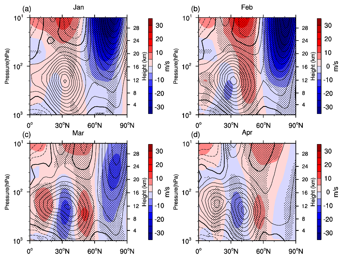
Figure 5.
Eddy momentum flux (color shading) during (a,d) WPV and (b,e) SPV events and (c,f) their differences (WPV minus SPV events) at (a–c) 300 hPa and (d–f) 700 hPa during January–February–March, as a function of the latitude and angular phase speed derived from the NCEP2 reanalysis data. The blue and red curve lines in each panel denote the zonal mean of the zonal wind (m/s) in January–February–March during WPV and SPV events, respectively.

Figure 6.
Probability distribution (unit: %) of the daily jet stream speed over the region of 65°–90° N and 170°–230° E (a) between 300 and 500 hPa and (b) between 700 and 850 hPa during January–February–March. (c),(d) are the same as (a,b), except for the region of 55°–65° N and 170°–230° E. Probability distribution (unit: %) of the daily jet stream latitude for the regions of 45°–90° N and 170°–230° E (e) between 300 and 500 hPa and (f) between 700 and 850 hPa. Blue and red lines and boxes represent WPV and SPV events, respectively.

Figure 7.
Composite differences between WPV and SPV events in March–April–May mean of SST derived from (a) the Hadley observation, (c) the CMCC-CMS historical simulation and (e) their differences (CMCC-CMS simulation minus Hadley data). Composite differences between WPV and SPV events in March–April–May mean of SLP (colorful shading) and 1000 hPa wind (vectors, unit: 1.5 m/s) derived from (b) the NCEP2 reanalysis data, (d) the CMCC-CMS historical simulation, and (f) their differences (CMCC-CMS simulation minus Hadley data). The differences over the dotted regions are statistically significant at the 95% confidence level according to Student’s t-test.

Figure 8.
Spatial patterns of the (a) EOF1 and (b) EOF2 modes of the North Pacific (20°–65° N, 125°–260° E) monthly sea surface temperature (SST) anomalies (after removing the monthly mean global average SST). (c) Daily mean PC1 (solid lines) and PC2 (dashed lines) from 1 February to 31 March during WPV (blue) and SPV (red) events. (d) Difference in the daily PC1 + PC2 index between WPV and SPV events from 1 February to 31 March.
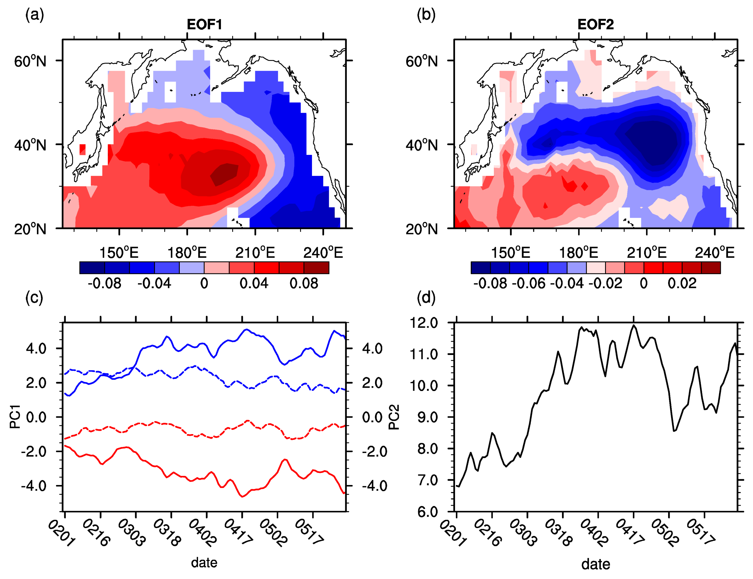
Figure 9.
Composite differences between WPV and SPV events in the average monthly rate of precipitation (contour lines, contour interval: 0.2 mm/day. The contour line and solid and dashed lines represent positive and negative values, respectively) and water vapor flux vector at 850 hPa (vector unit: 10−4 kg m/kg s)) during (a) February, (b) March, (c) April and (d) May. The differences over the dotted regions are statistically significant at the 95% confidence level according to Student’s t-test.

Figure 10.
Composite differences in 1000 hPa geopotential height over the North Pacific Ocean during (a) February, (b) March, (c) April and (d) May between WPV and SPV events with ENSO events excluded. The wind vectors represent the differences in 1000 hPa wind (unit: 1.5 m/s) between WPV and SPV events. The differences over the dotted regions are statistically significant at the 95% confidence level according to Student’s t-test.

© 2019 by the authors. Licensee MDPI, Basel, Switzerland. This article is an open access article distributed under the terms and conditions of the Creative Commons Attribution (CC BY) license (http://creativecommons.org/licenses/by/4.0/).
Share and Cite
MDPI and ACS Style
Zhang, K.; Wang, T.; Xu, M.; Zhang, J. Influence of Wintertime Polar Vortex Variation on the Climate over the North Pacific during Late Winter and Spring. Atmosphere 2019, 10, 670. https://doi.org/10.3390/atmos10110670
AMA Style
Zhang K, Wang T, Xu M, Zhang J. Influence of Wintertime Polar Vortex Variation on the Climate over the North Pacific during Late Winter and Spring. Atmosphere. 2019; 10(11):670. https://doi.org/10.3390/atmos10110670
Chicago/Turabian StyleZhang, Kequan, Tao Wang, Mian Xu, and Jiankai Zhang. 2019. "Influence of Wintertime Polar Vortex Variation on the Climate over the North Pacific during Late Winter and Spring" Atmosphere 10, no. 11: 670. https://doi.org/10.3390/atmos10110670
Note that from the first issue of 2016, this journal uses article numbers instead of page numbers. See further details here.