Article

A Climatological Satellite Assessment of Absorbing Carbonaceous Aerosols on a Global Scale

by
Nikolaos Hatzianastassiou
1,*,
Nikoleta Kalaitzi
2,3,
Maria Gavrouzou
1,
Antonis Gkikas
4,
Marios-Bruno Korras-Carraca
1,5 and
Nikolaos Mihalopoulos
6,7
1
Laboratory of Meteorology, Department of Physics, University of Ioannina, 45110 Ioannina, Greece
2
Department of Physics and Astronomy, University of Leicester, LE17RH Leicester, UK
3
Leicester Institute for Space and Earth Observation, University, of Leicester, LE17RH Leicester, UK
4
Institute for Astronomy, Astrophysics, Space Applications and Remote Sensing (IAASARS), National Observatory of Athens, 157 84 Athens, Greece
5
Department of Environment, University of the Aegean, 811 00 Mytilene, Greece
6
Institute for Environmental Research and Sustainable Development (IERSD), NOA, 11810 Athens, Greece
7
Environmental Chemical Processes Laboratory, Department of Chemistry, University of Crete, 70013 Crete, Greece
*
Author to whom correspondence should be addressed.
Atmosphere 2019, 10(11), 671; https://doi.org/10.3390/atmos10110671
Submission received: 29 August 2019 / Revised: 18 October 2019 / Accepted: 28 October 2019 / Published: 1 November 2019
(This article belongs to the Section Aerosols)

Abstract

:
A global climatology of absorbing carbonaceous aerosols (ACA) for the period 2005–2015 is obtained by using satellite MODIS (Moderate Resolution Imaging Spectroradiometer)-Aqua and OMI (Ozone Monitoring Instrument)-Aura aerosol optical properties and by applying an algorithm. The algorithm determines the frequency of presence of ACA (black and brown carbon) over the globe at 1° × 1° pixel level and on a daily basis. The results of the algorithm indicate high frequencies of ACA (up to 19 days/month) over world regions with extended biomass burning, such as the tropical forests of southern and central Africa, South America and equatorial Asia, over savannas, cropland areas or boreal forests, as well as over urban and rural areas with intense anthropogenic activities, such as the eastern coast of China or the Indo-Gangetic plain. A clear seasonality of the frequency of occurrence of ACA is evident, with increased values during June–October over southern Africa, during July–November over South America, August–November over Indonesia, November–March over central Africa and November–April over southeastern Asia. The estimated seasonality of ACA is in line with the known annual patterns of worldwide biomass-burning emissions, while other features such as the export of carbonaceous aerosols from southern Africa to the southeastern Atlantic Ocean are also successfully reproduced by the algorithm. The results indicate a noticeable interannual variability and tendencies of ACA over specific world regions during 2005–2015, such as statistically significant increasing frequency of occurrence over southern Africa and eastern Asia.

1. Introduction

Atmospheric aerosols can cause an overall planetary cooling, partly counterbalancing the global warming caused by greenhouse gases [1]. The total aerosol effective radiative forcing (ERF) taking into account aerosol–radiation and aerosol–cloud interactions (ERFari and ERFaci, respectively) is assessed to be −0.9 (−1.9 to −0.1) W m−2 with medium confidence [2]. More specifically, according to [1], the ERFari is assessed to be −0.45 (−0.95 to +0.05) W m−2, being less negative than in IPCCAR4th because of a reevaluation of aerosol absorption properties. In spite of the overall aerosol cooling, absorbing carbonaceous aerosols (ACA) including black carbon (BC) and brown organic carbon (BrOC) warm the planet. The BC aerosols dominated by soot-like elemental carbon (EC) are stronger absorbers of solar radiation than brown (BrOC), being also referred as brown carbon (BrC) aerosols, which mainly absorb at visible to ultraviolet wavelengths [3]. Both are primarily consisted of fine particles mostly less than 1μm [4,5,6] and together constitute ACA, which are estimated as the second largest source of global warming after carbon dioxide [7,8,9]. Apart from playing a major role in radiative forcing, aerosol solar absorption also has other effects, namely on atmospheric stability and circulation dynamics [10] photochemistry, visibility, health or on cloud properties through the aerosol indirect (cloud albedo effect, [11], cloud lifetime, [12]) and semi-direct [13,14,15] effects. Nevertheless, there is still considerable uncertainty about the magnitude of the global aerosol solar absorption and forcing [11,16,17]. This is largely attributed to the uncertainty associated with the spatial and temporal patterns of globally distributed ACA [18].
The ACA originate from both natural and anthropogenic sources and prevail over both urban areas [19,20,21,22,23] and continental outflow regions [24,25,26]. Biomass burning (BB) of both natural and anthropogenic origin is among the largest sources of ACA. In addition, activities taking place mainly over urban/industrial areas (UI aerosols), such as power plants emissions, industrial production, residential heating and cooking and transportation, are their main anthropogenic sources [27]. BB aerosols mainly occur over open continental areas, namely near to forest fires, but are also transported through atmospheric circulation to nearby continental and maritime areas. Regardless of their origin, both BB and UI ACA, despite their short lifetime [28], have a strong impact on climate, air quality [7,9] and are responsible for adverse health effects [29,30]. They can also cause biases in satellite retrievals of cloud optical properties, e.g., effective radius and optical depth [31,32,33] and therefore are worth studying. Consequently, it is essential to better understand their spatial and temporal variability as well as their global radiative and climate effects.
The global climatological assessment of ACA is a difficult task. A large number of studies exists dealing with the characterization of ACA [34,35,36,37,38,39]. However, these studies are based on ground based in-situ measurements and therefore are unable to ensure extended spatial coverage. ACA have also been identified at global scale using global models [40,41,42,43,44,45] which, however, have their own limitations. Remote sensing, especially satellite observations, which enable the identification and characterization of ACA at global scale, based on derived aerosol physical and optical properties, can provide important information regarding their spatial and temporal variability. Thus, many scientists have used satellite data in order to characterize aerosols and study their optical properties globally [46,47] or over broad areas, such as the Mediterranean basin [48,49], Europe [50], Atlantic Ocean [51], Middle East [52] and East Asia [53]. However, all of these studies do not exactly address the issue of observation, identification and quantification of ACA from a climatological and global perspective.
In the present study, for the first time to our knowledge, a satellite-based algorithm is used for characterizing/identifying ACA over the entire Earth and a multi-year period (2005–2015), allowing a climatological global assessment. A similar algorithm and satellite data have been previously applied by [54] to identify/characterize episodes of different aerosol types, carbonaceous included, above the greater Mediterranean basin for the period 2000–2007. In this study, a modified version of this algorithm is used along with updated satellite data (MODIS C006 instead of C005), focusing on ACA over the whole globe and an 11-year period. The algorithm uses daily gridded (1° × 1° latitude-longitude) satellite data from MODIS-Aqua describing the load (by means of AOD) and size of aerosols, and data from OMI describing the aerosol absorption ability and finally detects and quantifies ACA for each grid and day of the period 2005–2015. The presented results refer to the frequency of occurrence of ACA at global scale. The satellite data and algorithm are described in the next section. The analysis and obtained results are presented and discussed in Section 3, before summarizing and concluding in the last section.

2. Data and Methodology

2.1. MODIS and OMI Satellite Data

The aerosol data used as input to the algorithm, are part of MODIS Aqua spatiotemporally aggregated Level-3 daily gridded atmospheric data product (MYD08_D3). More specifically, Collection 006 (C006) MODIS Aqua aerosol data are used, which are generated by reprocessing MODIS data archives using calibration enhancements, algorithm refinements, and upstream product improvements [55,56] and have replaced the previous MODIS C005 data providing a better performance against AERONET data [57,58,59]. The following MODIS aerosol data describing the load and size of aerosols are used (as explained in Section 2.2) in the algorithm: (i) Aerosol Optical Depth (AOD), (ii) Ångström Exponent (a), and (iii) Fine Mode Fraction (FF) of AOD (the aerosol fine-mode fraction is defined as [60]: FF=AODf/(AODf + AODc), where AODf is the aerosol fine-mode optical depth and AODc is the aerosol coarse-mode optical depth). However, it should be noted that from them, only spectral AOD are directly taken from MODIS, while a (Ångström Exponent) and FF are derived from AOD. More specifically, AOD are taken from datasets produced with the MODIS Enhanced Deep Blue (DB) and Dark Target (DT) algorithms over land, and a DT algorithm over-water (ocean). The AOD data are available at 7 wavelengths over oceans (DT product) and 3 wavelengths over land (DT and DB products). Subsequently, Ångström Exponent data over land and ocean are computed from the spectral AOD values. Moreover, the fraction of AOD at 0.55µm contributed by fine mode aerosol (AODsmall) over oceans is available by MODIS (at 7 wavelengths). Computing the ratio of these AODsmall and AOD products provided FF over oceans. It should be noted that from the two MODIS data utilized in the algorithm, i.e., the a and FF, the former is available over land and ocean, whereas the latter is only available over ocean. Although it would be possible to only use a in the algorithm, over both land and ocean, it was preferred to additionally use FF over oceans, since FF is, by definition, slightly different to a, also depending, apart from size, on other aerosol properties, namely their concentration and refractive index. The use of different number of input parameters in the algorithm over land and ocean areas does not produce any discontinuity in the results, as shown in the next section.
Apart from MODIS, Aerosol Index (AI) (or Absorbing AI) daily gridded data are also used for the characterization of carbonaceous aerosols, derived from measurements taken by the Ozone Monitoring Instrument (OMI) instrument onboard the NASA’s EOS-Aura satellite since July 2004 [61]. These OMI-Aura satellite data are a sequel to those of Total Ozone Mapping Spectrometer (TOMS) onboard Nimbus-7 and Meteor-3 covering the period 01/1978–12/1994 and onboard Earth Probe satellite (EP-TOMS) launched in July 1996. OMI, similar to its predecessor TOMS, enables measurements and aerosol retrievals in the near-UV, including AI which is a unique qualitative parameter associated with the presence of UV absorbing aerosols (desert dust, smoke, volcanic ash). In the near-UV, the albedo of land surfaces (including arid and semiarid areas) is very low and, therefore, aerosol optical depth retrievals (full description provided by [62,63,64]) are possible over them. OMI, a hyperspectral sensor covering the 270–500 nm range, with its 2600 km viewing swath width provides almost daily global coverage at a 13 km × 24 km nadir resolution. OMI observations are used in the retrieval of atmospheric column ozone, sulfur dioxide, nitrogen dioxide, formaldehyde, and other trace gas, as well as cloud and aerosol information [65]. The OMI aerosol products apart from absorbing AI also include aerosol optical depth and single scattering albedo (388 and 500 nm) which have been carefully evaluated with AERONET observations [61,66,67,68,69,70,71]. In this study, only the AI index, which is a measure of aerosol absorptivity, is used and combined with the MODIS aerosol data.
The utilized MODIS-Aqua and OMI-Aura data are gridded daily products at 1°×1° latitude-longitude resolution data spanning the period from January 2005 to December 2015. It should be noted that MODIS-Aqua data were chosen for this study in order to ensure a collocation in time with OMI data, since Aqua and Aura are both A-train satellites, being in a polar orbit, crossing the equator northbound at about 1:30 p.m. local time, within seconds to minutes of each other, thus allowing near-simultaneous observations. The beginning of the study period is in 2005 because OMI data availability starts in this year. Earth Probe (EP) TOMS data are available prior to 2005, but OMI data were preferred in order to ensure the best homogeneity of the algorithm input satellite data during the entire study period (2005–2015).

2.2. Methodology

The flowchart of Figure 1 explains the structure of the algorithm and its operational phases. The combination of daily 1°×1° gridded MODIS and OMI data, which are indicative of aerosol load (AOD), size (a and FF) and absorptivity (AI), enable the identification/characterization of ACA aerosols, which are, as explained in sect. 1, small (fine) and strongly absorbing particles. Appropriate threshold levels were chosen for each one of the algorithm input aerosol optical properties used for the identification of ACA. The thresholds have been determined based on own sensitivity tests and the existing literature [72,73,74,75,76,77,78,79,80,81,82,83,84]. The selected/applied thresholds are: (i) a≥ 1.2 for Ångström Exponent, (ii) FF ≥ 0.6 for Fine Mode Fraction of AOD and (iii) АІ ≥ 1.5 for Aerosol Index. The obtained results of the algorithm using these thresholds confirm the presence of fine absorbing aerosols, which is the case for ACA.
The algorithm results are critically dependent on the OMI Aerosol Index (AI), since this parameter quantifies the required significant absorptivity of aerosols (their small/fine size is ensured by the other two optical properties, namely the Ångström Exponent, AE and the Fine Fraction, FF). The threshold value of AI (1.5), has been decided based on several sensitivity tests using AI thresholds ranging from 1.0 to 2.0. In Figure S1 (Supplement) are presented the results (annual frequency of occurrence of ACA, in number of days/year) of three (3) sensitivity tests for the (indicative) year 2005, using AI thresholds equal to 1.0, 1.5 and 2.0. The frequency of occurrence of ACA clearly decreases with increasing AI threshold values. With increasing AI from 1.0 to 2.0, not only the spatial coverage of areas with ACA is limited, but also the magnitude of the frequencies (intensity of green-yellow-red colours) is weakened. In the first sensitivity test, i.e., for AI=1.0, the presence of ACA is strong over extended continental areas, also covering considerably wide oceanic areas, even very far from the emission sources of ACA. Such a strong and extended presence of ACA is rather unrealistic. On the other hand, applying the threshold AI=2.0, the presence of ACA is drastically reduced, essentially resulting in their appearance only over the world continental areas dominated by strong and systematic forest fires, namely over South America and tropical and southern Africa. Such a limited presence of ACA is also somewhat unrealistic, since ACA, apart from elemental carbon from natural sources, consist in absorbing carbonaceous aerosols emitted by anthropogenic activities/sources and over urban areas, while (as shown in this paper) they can be transported over oceanic areas, for example reaching up to southeast Atlantic Ocean or South Ocean. The same results are confirmed by the corresponding monthly results of sensitivities, displayed in Figure S2. Therefore, the AI threshold value of 1.5 has been selected, which ensures the reasonable presence of ACA both over remote continental, urban, and also oceanic areas hosting natural and anthropogenic emissions of carbonaceous aerosols (as shown in Figure S1b, and also in Figure 3a in the followings).
The necessity of using other than AI input parameters to the algorithm, although suggested by the need to ensure the small/fine size of ACA, was verified running algorithm sensitivity tests using AI as the sole input parameter, and using additional parameters, namely Ångström Exponent and FF. The results of this sensitivity test, i.e., the absolute frequency of occurrence of ACA, again for the test year 2005, are displayed in Figure S3 and are to be compared to those of Figure S1b. The ACA frequencies of Figure S3 totally differ from those of Figure S1b. Very high frequencies, up to 344 days/year, are obtained, while the highest ACA frequencies estimated by the algorithm are found over North Africa, namely over the Sahara desert, as well as over the deserts of Arabian peninsula, essentially corresponding to dust aerosols, and not to carbonaceous ones. Hence, the regions hosting extended biomass burning, e.g. African and South American forests, do not distinctly appear on the map. This result proves the inability of the sole AI parameter for the detection of ACA globally, and the appropriateness of an algorithm like the one utilized in this paper, which is relied on other than AI products as well, which ensure the fine size of absorbing aerosols, namely Ångström Exponent and FF.
As already mentioned in Section 2.1, the use of FF as input parameter in our algorithm, which is available only over ocean, may be a source of discontinuities and land/sea contrast. In fact, the use of a single size parameter over land areas (Ångström Exponent, along with AI), against two parameters over ocean (Ångström Exponent and FF, still along with AI) may produce a difference in the algorithm outputs (frequency of ACA) over land and ocean areas, producing discontinuities along the coastlines. This was examined running a sensitivity test with the algorithm, using either both Ångström Exponent and FF or only FF. The sensitivity was made again for the year 2005, and the results are shown in Figure S4. It is shown that when we omit FF (Figure S4b), the obtained results, i.e., frequencies of ACA, do not essentially differ from those obtained using both AE and FF (Figure S4a). The spatial patterns and coverage of ACA dominated regions, as well as the magnitude of ACA frequencies are well comparable. The only difference is that using only Ångström Exponent a slightly more limited spatial coverage of ACA areas is found, along with just slightly smaller frequencies(by up to 5–10 days/year). Similar results are obtained, and same conclusions are drawn, by looking at the same sensitivity but on a monthly basis (Figure S5). Given the very small differences between the two examined cases in this sensitivity test, it was preferred to keep using both Ångström Exponent and FF as input parameters to the algorithm.
Note that low carbon content ash emitted during volcanic eruptions, which is also fine [85] and possibly absorbing [86], may be accounted for by the algorithm outputs, but it is not persistent in the atmosphere, and hence its contribution to the 11-year averaged results presented in this study is minimal. It should be noted that this algorithm detects carbonaceous aerosols using three (3) aerosol optical properties, i.e., a, FF and AI, while previous studies [47,87] use only one property, more specifically the AI. The selection of AI threshold 1.5 was made in order to ensure the identification of ACA that occur over the globe, namely over or close to forest wildfires, e.g., in Amazonia and central Africa, or near extensive biomass-burning activities/areas [88,89]. In such cases, emissions of carbonaceous aerosols are very strong [90] and these aerosols predominate throughout the atmospheric column [91,92] yielding a strong absorption of solar radiation. It should be noted that the aerosol data used in the present algorithm are columnar, and therefore identification of ACA presupposes the prevalence of these aerosols in the atmospheric column, thus the obtained results should be interpreted in this aspect. In other words, the identification of ACA over a world location in a given day does not imply that only ACA exist in the overlying atmosphere, but just that ACA dominate the atmospheric columnar aerosol burden in terms of the aerosol optical properties utilized in the algorithm, especially the AI.
The algorithm identifies the presence of ACA in each day of the period 2005–2015. Subsequently, statistics are yielded for each month and year, including the monthly and annual absolute frequency of occurrence of ACA, N (in number of days per month/year) and the monthly and annual relative frequency of occurrence of ACA Nrel (in number of days per month/year per the number of days per month/year for which the satellite algorithm operated). Although the algorithm operates at the global scale, emphasis is also given to specific world regions, which are characterized by extensive fires and biomass burning, and computations (averaging) of the frequency of occurrence and the loading of ACA are also done for these regions. Such a region is for example southern Africa, which hosts the largest biomass-burning emissions, with an average 23% of the global burned area and 23% of the global fire emissions [88,93,94]. ACA from southern Africa are also transported westwards above the Atlantic Ocean [95,96,97]. In South America, large forest areas are burned each year with an average of 5% of the global burned area and 13% of the global fire emissions [84]. Central Africa also has high ACA emissions due to extended burnt savanna areas during December till February [98]. Other areas of interest, though with lower emissions of ACA and less biomass burning [99,100] are equatorial Asia (Indonesia and Malaysia), East Asia (including eastern Asiatic part of Russia and northeastern China), and Southeast Asia. The selected study areas are presented in Figure 2.

3. Results and Discussion

The algorithm ran on a daily basis and for each year of the study period (2005–2015). The outputs were then averaged over each month and year, and finally over the entire 11-year period. Below are presented11-year averaged monthly quantities, namely frequency of occurrence of ACA.

3.1. Geographical Patterns of Carbonaceous Aerosols
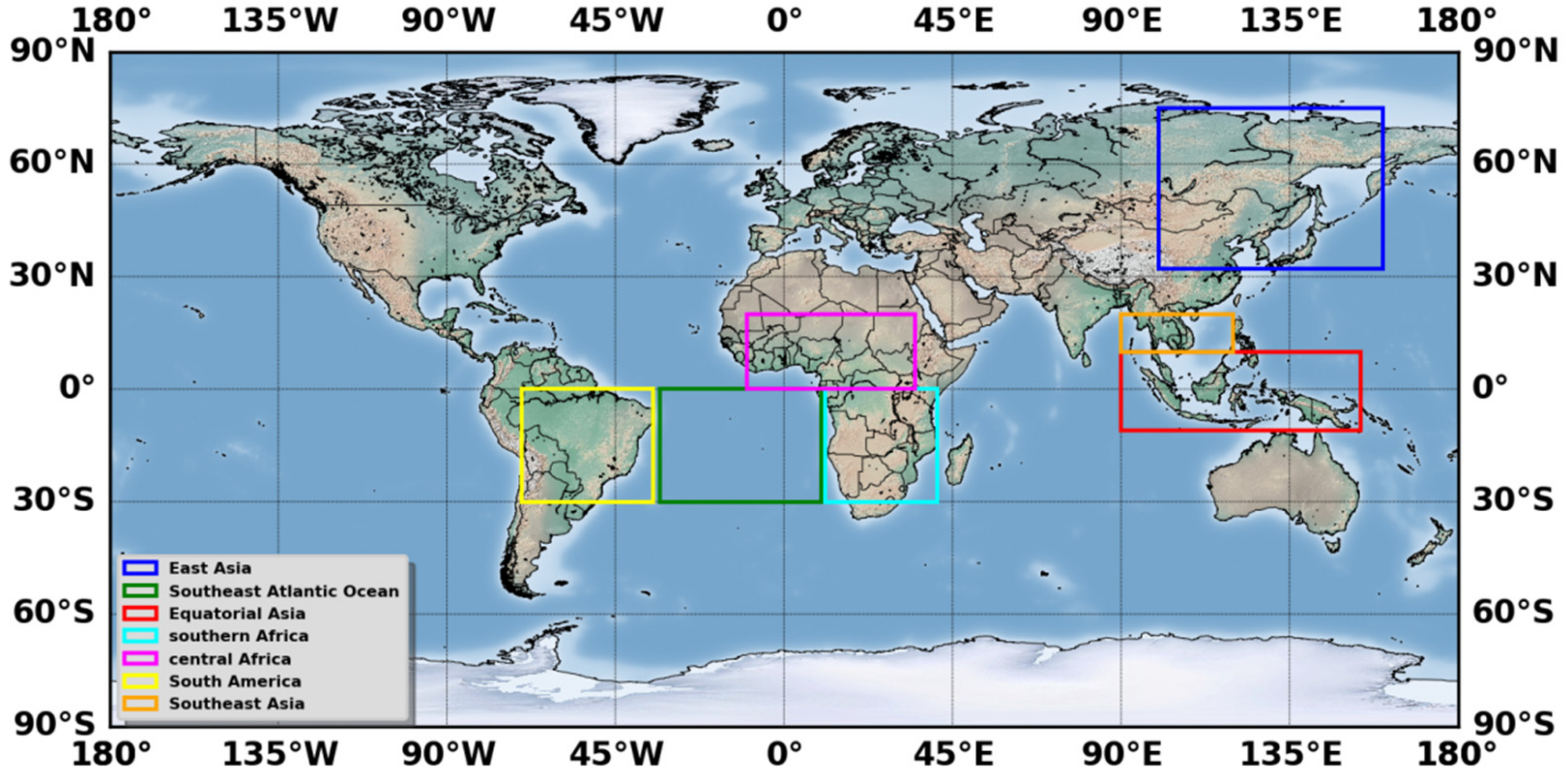
The global distribution of the absolute annual frequency of occurrence of ACA (in days/year) averaged for the entire period 2005–2015 is given in Figure 3a. In Figure 3b is also displayed the relative percentage annual frequency of occurrence of ACA with respect to the number of days in a year for which the algorithm operated. White shaded areas in the figures correspond to cases (pixels) for which the algorithm never operated (non-operating algorithm) or detected ACA (non-detecting ACA). The similarity between Figure 3a,b indicates that the spatial patterns in absolute frequency of ACA are not dominated by data availability from MODIS or OMI. Similar results to those of Figure 3a, i.e., absolute frequency of occurrence of ACA, but on a monthly basis, expressed in days/month, are displayed in Figure 4 and they are discussed together with those of Figure 3.

3.1.1. Africa

The highest frequencies of ACA occur in southern African countries, especially over Angola and Congo, where ACA predominate in about 60 days/year (or 50%, Figure 3a). These high frequencies, which are observed from May to October, with frequencies up to 19 days/month (Figure 4), and with maxima in July–August, are due to the extensive burning activities that take place every year in these regions, and they are related with agricultural burning (dry grass and vegetation fires) and wildfires occurring in large and dense forest areas [101]. Indeed, a prolonged annual dry season (May–October) combined with relatively rapid rates of fuel accumulation create conditions conducive to frequent vegetation fires in southern Africa’s savanna (woodland) and grassland vegetation types [102,103,104,105]. It is known that African fires, most of them coming from African areas south of the equator, account for 72% of the global burned area, making Africa the largest biomass-burning emissions source, contributing over half (52%) of the global carbon emissions [106]. It should be noted that high frequencies of ACA (almost up to 50 days/year) are also observed over the south eastern Atlantic Ocean, off the western coasts of African countries (Angola, Congo, Gabon). These are associated with an effective westward transport of African biomass aerosols convectively uplifted to the free troposphere, and subsequently transported westward (e.g., up to the Ascension Island 2000 km offshore the continental Africa) by a well-established anticyclonic circulation induced by the semi-permanent sub-tropical anticyclone of the South Atlantic [97]. Smaller frequencies of ACA (up to about15–20 days/year, Figure 3a) are observed in Central Africa (between the equator and sub-Sahel). These are more specifically observed from December to April (Figure 4), with frequencies up to about 9 days/month (maxima in December and January),and originate from fires taking place over shrubland and cropland areas between November and April [98,101,107,108].Very low frequencies of occurrence of ACA, lower than 5–10 days/year (on an 11-year basis), are found over the Sahara. Such low frequencies of ACA aerosols over this world region have been reported in the literature [109,110,111] and are associated with a northward transport of biomass-burning aerosol (emitted by anthropogenic activities south of 11°N) in warm ascending air that overrides the cooler, drier mineral dust laden air, reaching altitudes higher than 4 km [109].

3.1.2. South America

ACA occur frequently in South America, mainly its southern hemispherical part, in up to about 30 days/year (Figure 3a) or up to 35–40% of the days in which the algorithm operated (Figure 3b). These high frequencies are related to landscape fires and open biomass burning, with regional hotspots of fire activity around the edges of Amazonia [112], take place during the dry season (June to October, [113]) with peak fire activity in August and September [88,101], as shown in Figure 4. This biomass-burning activity results in extended burned areas each year (12.8 Mha/year on average, [88]). The seasonality of the algorithm outputs for this world region and more specifically over the Amazonian basin is in agreement with other studies [2,112]. It can be noticed that over the white shaded areas of northern–northeastern South America there are sparsely distributed greenish-yellowish-reddish pixels indicating that ACA are observed there with relative percentages higher than 40%. These high frequencies are associated with Amazonian forest fires, which although they are less frequent than in the rest of South America [88] they have very high fire emissions per m2 of burned area and constitute a strong source of carbon emissions worldwide [106]. ACA are also observed along the Andes (coasts of Peru and Chile), with relative frequencies up to about 30–40% in southern Peru. Although fire and carbon emissions are generally low over both of these areas [88,106], fires and biomass burning are common in the Andes, especially the tropical fires during the dry season of the year [114]. It should be noted that aerosol black carbon enhanced concentrations from urban/industrial origin in South America can be transported to the South–West Atlantic Ocean [115,116], which can explain the low frequencies of ACA observed near the South Pole rime (Figure 3a,b).

3.1.3. Asia

Relatively high frequencies of ACA (up to about 25 days/year, light blue-green colors) are also observed in south-southwestern Asian countries (Turkmenistan, Afghanistan, Pakistan, Nepal) as well as in the eastern/coastal China (maximum values up to about 30–35 days/year near Beijing). The corresponding computed relative frequencies (Figure 3b) display clearly high values (40–80%, green-yellow-red pixels) in south-southwestern Asian countries and in the south-southeastern Tibetan plateau, as well as in the northern Indo-Gangetic plain. A careful look at Figure 4 indicates that these high frequencies occur in winter (November–December–January–February) and spring (March–April–May). The relatively high frequencies of ACA over these regions are related either to biomass burning, more specifically burning of agricultural residues and grassland, that take place from winter through to spring [117,118] or to other anthropogenic activities like coal combustion, [119]. The strong presence of ACA over South Asia, especially over the Indo-Gangetic plain, is well documented in literature and plays an important role for south Asian climate and hydrological cycle [120,121]. It should be noted that according to the literature [106,117,122], strong biomass burning, also occur over the southeastern Asia, which is reported to be a significant contributor of annual global biomass-burning emissions (6%, [72,85]). Indeed, according to the algorithm results, considerable frequencies of ACA (up to 25–30 days/year or 40%, Figure 3a,b, respectively) are observed over Myanmar and Thailand during winter and spring (from February to April, Figure 4). These results are in agreement with the strong fire activity persisting from January to April reported in the literature [122]. The ACA over the southeastern Asia originate primarily from savanna burning (almost 60 % of burned areas there, [123]), and also from forest and cropland burning (20 % each).

3.1.4. Equatorial Asia

Large frequencies of occurrence of ACA are observed over equatorial Asia (Indonesia) which is reported to be the third largest contributor of annual biomass burning and fire emissions (11% and 10 %, respectively, [88,96]) after Africa (49 % and 52 %) and South America (13% and 15 %). The high frequencies over equatorial Asia are more evident in Figure 3b, reaching about 60–70% of the days of year for which the algorithm operated. They are in line with high annual fire carbon emissions in equatorial Asia reported in the literature [96] arising from numerous forest fires, but also savanna and cropland fires, and from extended burned areas [122,123]. Indeed, large numbers of active fires have been reported over Indonesia from August until October [122] in agreement with the monthly results of the algorithm (Figure 4, frequencies up to 8–9 days/month). It should be noted that the algorithm year-by-year results (not shown here) reveal a strong interannual variability, primarily associated with the fact that fire activity within equatorial Asia–Indonesia is strongly associated with El Niño Southern Oscillation (ENSO) events [124,125], with more burned areas during warmer and dry El Niño than cooler and wet La Niña phases [122]. This interannual variability is presented in Section 3.2, where the year-to-year variability of the regionally averaged algorithm results for equatorial Asia–Indonesia is shown (Figure 5 and Figure 6).

3.1.5. Boreal America, Boreal Asia, central America and Australia

ACA are also observed along the temperate North America (USA), with frequencies up to about 20 days/year in western USA, and can be explained from fires taking place therein [122]. Of course, the presence of ACA in temperate North America, e.g., in local winter, can also be related to anthropogenic ACA primarily emitted from incomplete combustion of fossil or biomass fuels [126,127] or secondarily formed from combustion emissions [128].
ACA are also observed at relatively high frequencies over boreal Asia, i.e., area north of about 50°N (up to about 20 days/year or 40–50% of days for which the algorithm operated, Figure 3a,b, respectively). This region has a considerable fire activity taking place from March to October [101,122,123]. These are mostly forest fires that are quite persisting (1 to 1.5 days per month, [129]) burning extended areas (about 15 Mkm2, [90], or up to about 10% of total areas each year, [123]). These forest fires lead to significant carbon emissions (up to 200 g carbon m−2 year−1, [106]) which are almost 2.5 times as high as those from boreal North America and comparable to emissions from Australia [106] and contribute about 6.5% of average annual global biomass-burning emissions [88]. Such biomass-burning emissions can undergo intercontinental transport and reach western North America [130]. The findings of the algorithm (Figure 4), which show high frequencies of ACA in the period March–October, and a maximum frequency of ACA in July and August (about 5–10 days/month) are in agreement with the seasonality of fires activity in boreal Asia reported in the literature.
Relatively large absolute frequencies of ACA are observed in Australia, with maximum values in its northern and central parts (up to about 30 days/year, Figure 3a). These are related to active fires, and resulted burned areas, occurring primarily in savanna, and also in shrubland and grassland areas across northern Australia throughout the year, but mainly in September, October and November [122,123] in agreement with the monthly results of the algorithm, which reveal frequencies up to 8 days/month (Figure 4).

3.2. Intra-Annual and Interannual Variability of ACA

The seasonal variability of the frequency of occurrence and loading of ACA over specific world areas of interest has already been discussed in the previous Section 3.1. Nevertheless, this is by nature much easier to do by focusing and spatially averaging over the areas of the specific regions. This was done for the seven (7) selected world regions specified in Section 2, namely: central Africa, southern Africa, South America, southeastern Atlantic Ocean, equatorial Asia, East Asia, and southeastern Asia. The seasonality of ACA over each one of these regions is presented in Section 3.2.1, whereas their interannual variability is examined in Section 3.2.2.

3.2.1. Intra-Annual Variability

Figure 5 displays the 11-year average frequencies of occurrence of ACA (in number of pixel or counts/year) over the selected 7 world regions along with the associated standard deviation which quantifies the year-to-year variability. The corresponding year-by-year results are presented in Figure 6. The computed results in number of pixel or counts/year can be compared with other products, such as for example fire occurrences or activity or biomass burning fuels or emissions. Although some seasonality is more or less evident in all regions apart from East Asia, it is more distinct in regions, such as central Africa, southern Africa, southeastern Asia and southeastern Atlantic Ocean, whereas it is much weaker over East Asia, South America or equatorial Asia. Over the latter two regions the magnitude of frequency during the peak seasons varies remarkably from a year to another, even approaching zero values in some years (Figure 6iii,v). The highest frequencies of occurrence of ACA (3000 counts/year on average, Figure 5ii) are observed over southern Africa as well as over the southeastern Atlantic Ocean (2300 counts/year on average, Figure 5iv) from June to October with peak frequencies usually occurring in August and September and rarely in July. As already reported in Section 3.1, these high frequencies are due to frequent vegetation fires in southern Africa’s savanna and grassland vegetation types. The produced ACA are frequently transported westwards over the southeastern Atlantic Ocean, following a similar seasonality with those from southern Africa. Besides, there is a considerable interannual variability during the peak season (Figure 5ii for southern Africa and Figure 5iv for SE Atlantic Ocean).
The second-highest frequencies of occurrence of ACA are observed over Central Africa (Figure 5i) from December to April, when intense fire activity takes place over shrubland and cropland areas (see Section 3.1). The results of Figure 5iv reveal the existence of a secondary, but much lower, maximum frequency of occurrence period in Central Africa, which lasts from June to August, i.e., during the wet season over the area [131,132]. The existence of this secondary maximum could be explained by the presence of ACA transported by the monsoon flow originating in Southern Africa, a region with large biomass burning sources [133].
Another region with a distinct seasonality is South America, where ACA occur frequently (up to 1100 counts/year, Figure 5iii) from June to October, with maximum frequencies in August, which are however characterized by a great interannual variability. The peak frequencies over this region, which arise from landscape fires and open biomass burning associated with deforestation and agricultural activities, largely vary from a year to another, e.g., from as few as 200counts/year in 2014 to 3500 counts/year in 2007, Figure 6iii).
The results of Figure 5vii reveal a clear seasonality of ACA frequency of occurrence over southeastern Asia, which is higher (up to 1000 counts/year on average) from January to April, peaking in March and April, yet with a considerable year to year variability, due to forest and savanna fires.
Over equatorial Asia (Figure 5v), ACA are most frequently observed in September and October (150 counts/year on average), but with quite variable frequencies of occurrence (ranging from a few tens of counts/year (e.g., in 2011, 2012, 2013) up to 850 counts/year (in 2015), annual results Figure 6v) which are associated with large error bars. The great interannual variability of ACA frequency of occurrence in equatorial Asia is in agreement with other studies [122,123,125,134]. A great year to year variability of ACA frequencies is also observed for East Asia, which is characterized by the absence of a specific seasonality.

3.2.2. Interannual Variability

The interannual variation of the mean annual frequency of ACA over the selected 7 study world regions is presented in Figure 7. The estimated linear trends during 2005–2015, as well as their statistical significance (ascertained from the computed standard error of the slope of the applied linear regression), are also presented for each region in Figure 7.
From the results of Figure 7, it is gathered that the presence, i.e., frequency of occurrence, of ACA has been more or less intensified from 2005 to 2015 over all the selected world regions except for South America (where a no statistically significant decreasing trend is found). Furthermore, it appears that the increasing trend is statistically significant only over 2 regions, namely over southern Africa and East Asia. The highest percent increase in frequency of occurrence is found for equatorial Asia (151.1%, though this is largely due to the very high frequency value in 2015) and East Asia (122.2%) followed by the increase in southern Africa (59.3%) while smaller increases are observed over the southeastern Atlantic Ocean (34.8%). The remarkably strengthened presence of ACA over the East Asia can be assigned to a large degree to the continued consumption of fuels like coal and diesel during 2005–2015 [135]. The increasing frequency of occurrence of ACA over southern Africa during 2005–2015 (Figure 7i) seems to be in line with the reported increase of burned areas till 2012 [105]. According to our results, the presence of ACA in southern Africa has intensified even more from 2012 to 2015. Concerning equatorial Asia, it can be noted that the overall increase essentially arises from the very high frequencies in 2015, against low frequencies before and especially before 2013 (Figure 7v). If the high 2015 frequencies are excluded, a decline is estimated for equatorial Asia, which is in line with reported decreasing burned areas over the equatorial Asia till 2012 [123]. Apart from 2015, high frequencies of ACA over equatorial Asia are also found in 2006, and much less in 2009, which are in line with strong warm and dry El Nino phases in those years. Indeed, values of Nina-4 Index anomalies for those years (not shown here), and especially for September, October and November, when high frequencies of ACA are detected by the algorithm (Figure 7v), reach up to 0.8 (2006), 1.2 (2009) and 1.6 (2015), indicating warm and dry El Nino conditions. The results of the algorithm are in agreement with literature reporting that fire activity and burned areas within equatorial Asia are strongly associated with ENSO events [124,125]. The obtained algorithm results span the period 2005–2015, and therefore it is difficult to be compared to relevant results from other studies, which mostly stop at 2010. Nevertheless, comparing the present results, i.e., interannual variability and trends, spanning the years till 2010 to relevant reports in literature, e.g., burned areas [122] or fire carbon emissions [106], a very good agreement for the studied world areas is found.

4. Conclusions

A satellite-based algorithm is used to build, for the first time to our knowledge, a climatology (for the 11-year period 2005–2015) of the frequency of occurrence of absorbing carbonaceous aerosols (ACA). The algorithm uses MODIS-Aqua and OMI-Aura satellite retrievals of key aerosol optical properties, namely Ångström exponent (a), fine fraction (FF) and absorption index (AI). Applying specific thresholds for these properties, fine and absorbing carbonaceous aerosols either of natural or anthropogenic origin are detected on a daily basis and at 1° × 1° latitude-longitude pixel-level over the globe. The frequency of presence of ACA was computed first on a daily basis, and then on a monthly and annual mean basis, while corresponding regional averages for specific world areas of interest were also computed.
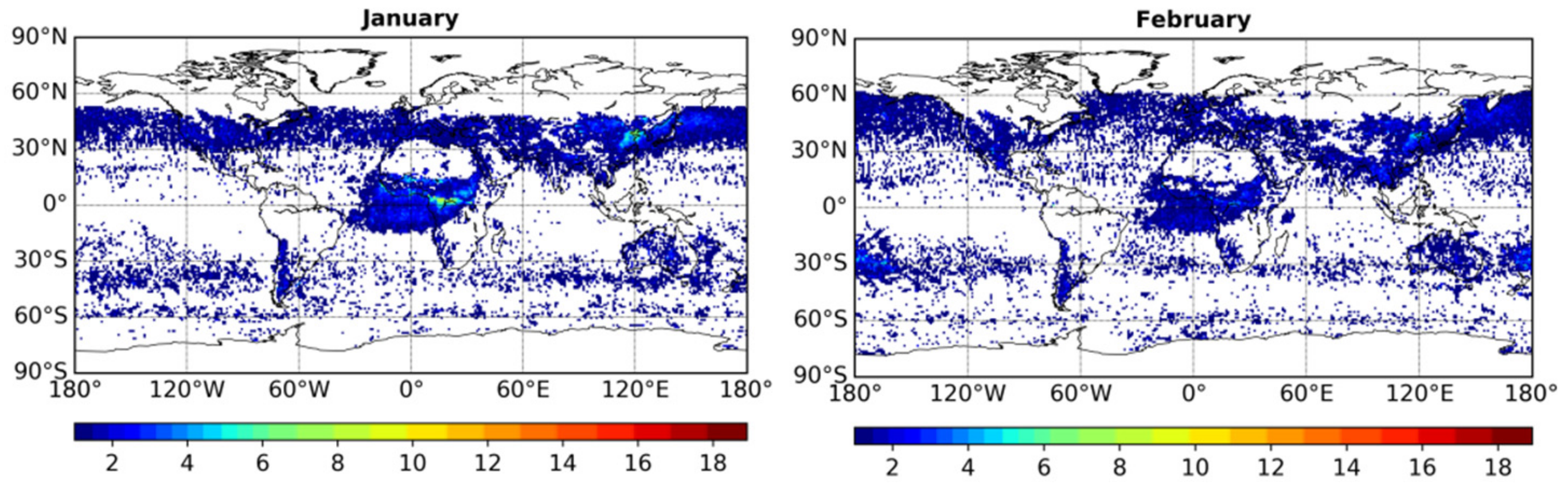
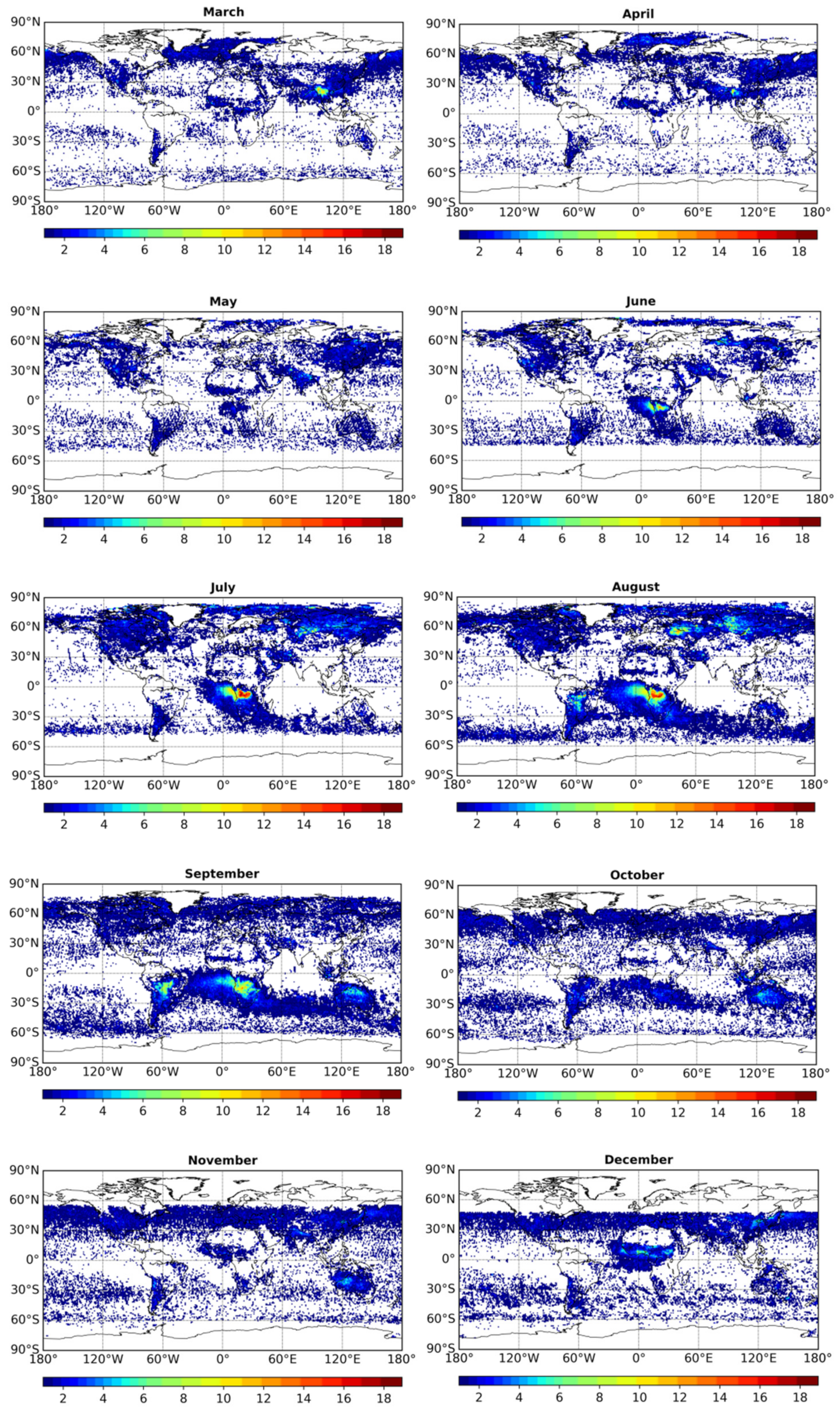
  • The results of the algorithm reveal that on average, ACA are observed over the globe up to about 80 days per year. Their largest frequencies are found in southern Africa, where they occur in about 30–80 days/year over Angola and Congo, as well as over the southeastern Atlantic Ocean, where they arrive after traveling for thousands of kilometers from the aforementioned areas of southern Africa. Relatively high frequencies of ACA are also found over the southern hemispherical part of South America (up to 30 days/year), equatorial Asia (Indonesia, Malaysia), over the southern-southeastern parts of Asia and the eastern coast of China as well as over the northern and central Australia (up to 30 days/year). Lower frequencies are identified over central Africa, between the equator and sub-Sahel (15–25 days/year), and over boreal Asia and the temperate North America (up to 30 days/year). As the algorithm did not operate in all days of each year, because not all of its input data were available, the above mentioned frequencies practically refer to less than 365 days of the year, thus yielding higher relative percent frequencies of occurrence of ACA. For example, ACA are observed in 50% of the days for which the algorithm operated over the southern African areas of Angola and Congo, 35–40% of days over South America or 40–80% over south-southwestern Asian countries, the south-southeastern Tibetan plateau, and the northern Indo-Gangetic plain, while they are observed in about 60–70 % of the days of year in which the algorithm operated over equatorial Asia (Indonesia).
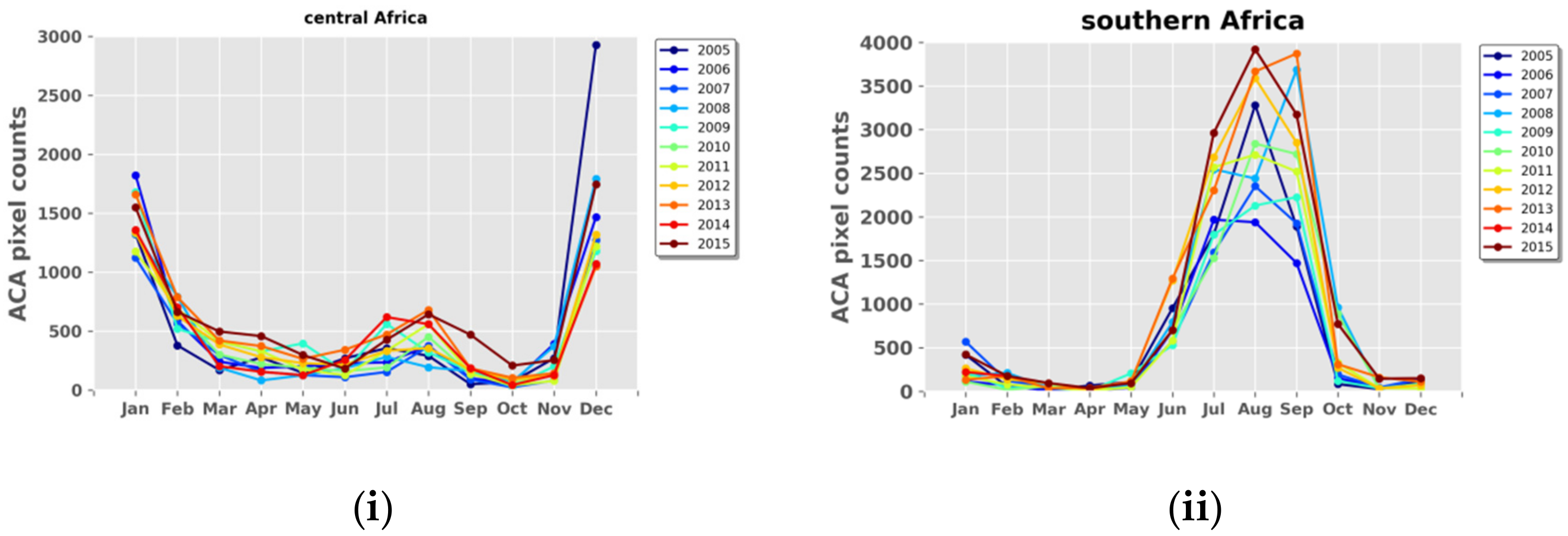
  • The algorithm results reveal a seasonality of the frequency of occurrence of ACA, which is in line with the known seasonal cycles of burning processes, namely agricultural burning (dry grass and vegetation fires), intensive livestock activities, and wildfires in large and dense forest areas, worldwide. The highest frequencies of ACA over southern Africa, its adjacent southeastern Atlantic Ocean, and South America take place during the local dry season, namely during May to October—with maxima in July–September—in the former two regions and June to October—with maxima in August–September—in the latter region). Equatorial Asia (Indonesia) and Southeast Asia exhibit a distinct seasonality with highest frequencies of ACA in late autumn (September–October) for the former and spring (March–April) for the latter. Finally, in Central Africa, the annual maximum frequencies are observed in December and January, while secondary maxima are found in July–August.
  • A rather predominant and strengthened presence of ACA over extended global regions is indicated by the results of the algorithm. This can have important climate implications given the strong solar absorbing ability and heating potential of these aerosols [11], which are considered to be the secondary (to carbon dioxide) warming driver of the contemporary global climate [1,9,136]. Apart from climate effects, the more frequent presence of ACA during 2005–2015 has also deteriorated air quality, and caused premature deaths worldwide and especially in East and South Asia [137], where according to our results the highest and statistically significant at 95% level increase of frequency is observed.
In the future, an improvement of the algorithm will be the ability to determine the fraction of AOD that is only attributed to ACA. This is a difficult task, since it requires the knowledge of the detailed vertical distribution of different aerosol types (ACA included) on a detailed, but at the same time complete, temporal (daily, multi-year) and spatial (1° × 1°, global) resolution, which is missing nowadays. Nevertheless, forward steps are made towards this direction (e.g., Cloud-Aerosol Lidar with Orthogonal Polarization, CALIOP) and the situation is expected to improve in the forthcoming years.

Supplementary Materials

The following are available online at https://www.mdpi.com/2073-4433/10/11/671/s1, Figure S1: Global distribution of the annual absolute frequency of occurrence of absorbing carbonaceous aerosols (in number of days/year) for AI thresholds equal to 1.0 (a), 1.5 (b) and 2.0 (c). The results are for the year 2005., Figure S2. Global distribution of the monthly absolute frequency of occurrence of absorbing carbonaceous aerosols (in number of days/month) for AI thresholds equal to 1.0 (left column), 1.5 (middle column) and 2.0 (right column). Each row corresponds to the months of the year, from January (top) to December (bottom). The results are for the year 2005. Figure S3. Global distribution of the absolute frequency of occurrence of absorbing carbonaceous aerosols (in number of days/year) computed using as unique criterion in the algorithm the AI threshold value of 1.5. The results are for the year 2005. Figure S4. Global distribution of the absolute frequency of occurrence of absorbing carbonaceous aerosols (in number of days/year) computed using as input parameters (apart from AI) Ångström Exponent and Fine Mode Fraction (a) and Ångström Exponent only (b). The results are for the year 2005. Figure S5. Global distribution of the monthly mean absolute frequency of occurrence of absorbing carbonaceous aerosols (in number of days/year) using either both Ångström Exponent and Fine Mode Fraction (left column) or Ångström Exponent only (right column) as input parameters to the algorithm (along with AI). Each row corresponds to the months of the year, from January (top) to December (bottom). The results are for the year 2005.

Author Contributions

Conceptualization, N.H.; methodology, N.H. and A.G.; software, N.H. and N.K.; investigation, N.H., M.G. and N.K.; resources, N.H.,N.K. and M.G.; data curation, N.H.,N.K. and M.G.; writing—original draft preparation, N.H.; writing—review and editing, N.H., A.G., M.G. and N.M.; visualization, A.G., M-B.K-C.; supervision, N.H.; project administration, N.H. and N.M.; funding acquisition, N.H. and N.M.

Funding

This research received no external funding. The APC was funded by the project “Panhellenic Infrastructure for Atmospheric Composition and Climate Change” (MIS 5021516), which is implemented under the Action “Reinforcement of the Research and Innovation Infrastructure”, funded by the Operational Programme “Competitiveness, Entrepreneurship and Innovation” (NSRF 2014-2020) and co-financed by Greece and the European Union (European Regional Development Fund). Τhis work is part of ACTRIS-2, which has received funding from the European Union’s Horizon 2020 research and innovation programme under grant agreement no. 654109.

Conflicts of Interest

The authors declare no conflict of interest.

References

  1. IPCC. Climate Change 2013: The Physical Science Basis. Contribution of Working Group I to the Fifth Assessment Report of the Intergovernmental Panel on Climate Change; Stocker, T.F., Ed.; Cambridge University Press: Cambridge, UK; New York, NY, USA, 2013; 1535p. [Google Scholar]
  2. Artaxo, P.; Rizzo, L.V.; Brito, J.F.; Barbosa, J.M.; Arana, A.; Sena, E.T.; Cirino, G.G.; Bastos, W.; Martin, S.T.; Andreae, M.O. Atmospheric aerosols in Amazonia and land use change: From natural biogenic to biomass burning conditions. Faraday Discuss. 2013, 165, 203–235. [Google Scholar] [CrossRef] [PubMed]
  3. Bahadur, R.; Praveen, P.S.; Xu, Y.; Ramanathan, V. Solar absorption by elemental and brown carbon determined from spectral observations. Proc. Natl. Acad. Sci. USA 2012, 109, 17366–17371. [Google Scholar] [CrossRef] [PubMed] [Green Version]
  4. Offenberg, J.H.; Baker, J.E. Aerosol size distributions of elemental and organic carbon in urban and over-water atmospheres. Atmos. Environ. 2000, 34, 1509–1517. [Google Scholar] [CrossRef]
  5. Streets, D.G.; Bond, T.C.; Lee, T.; Jang, C. On the future of carbonaceous aerosol emissions. J. Geophys. Res. 2004, 109, D24212. [Google Scholar] [CrossRef]
  6. Viidanoja, J.; Kerminen, V.M.; Hillamo, R. Measuring the size distribution of atmospheric organic and black carbon using impact or sampling coupled with thermal carbon analysis: Method development and uncertainties. Aerosol Sci. Technol. 2002, 36, 607–616. [Google Scholar] [CrossRef]
  7. Bond, T.C.; Doherty, S.J.; Fahey, D.W.; Forster, P.M.; Berntsen, T.; De Angelo, B.J.; Flanner, M.G.; Ghan, S.; Kärcher, B.; Koch, D.; et al. Bounding the role of black carbon in the climate system: A scientific assessment. J. Geophys. Res. 2013, 118, 5380–5552. [Google Scholar] [CrossRef]
  8. IPCC. Climate Change 2014: Impacts, Adaptation, and Vulnerability. Part A: Global and Sectoral Aspects, Contribution of Working Group II to the Fifth Assessment Report of the Intergovernmental Panel on Climate Change; Field, C.B., Barros, V.R., Dokken, D.J., Eds.; Cambridge University Press: Cambridge, UK; New York, NY, USA, 2014. [Google Scholar]
  9. Ramanathan, V.; Carmichael, G. Global and regional climate changes due to black carbon. Nat. Geosci. 2008, 1, 221–227. [Google Scholar] [CrossRef]
  10. Samset, B.H.; Stjern, C.W.; Andrews, E.; Kahn, R.A.; Myhre, G.; Schulz, M.; Schuster, G.L. Aerosol Absorption: Progress Towards Global and Regional Constraints. Curr. Clim. Chang. Rep. 2018, 4, 65–83. [Google Scholar] [CrossRef] [Green Version]
  11. Twomey, S. Influence of pollution on shortwave albedo of clouds. J. Atmos. Sci. 1977, 34, 1149–1152. [Google Scholar] [CrossRef]
  12. Albrecht, B.A. Aerosols, cloud microphysics, and fractional cloudiness. Science 1989, 245, 1227–1230. [Google Scholar] [CrossRef]
  13. Hansen, J.; Sato, M.; Ruedy, R. Radiative forcing and climate response. J. Geophys. Res. 1997, 102, 6831–6864. [Google Scholar] [CrossRef]
  14. Koch, D.; Del Genio, A.D. Black carbon semi-direct effects on cloud cover: Review and synthesis. Atmos. Chem. Phys. 2010, 10, 7685–7696. [Google Scholar] [CrossRef]
  15. Jacobson, M.Z. Investigating cloud absorption effects: Global absorption properties of black carbon, tar balls, and soil dust in clouds and aerosols. J. Geophys. Res. 2012, 117, D06205. [Google Scholar] [CrossRef]
  16. Stier, P.; Seinfeld, J.H.; Kinne, S.; Boucher, O. Aerosol absorption and radiative forcing. Atmos. Chem. Phys. 2007, 7, 5237–5261. [Google Scholar] [CrossRef] [Green Version]
  17. Wang, X.; Heald, C.L.; Ridley, D.A.; Schwarz, J.P.; Spackman, J.R.; Perring, A.E.; Coe, H.; Liu, D.; Clarke, A.D. Exploiting simultaneous observational constraints on mass and absorption to estimate the global direct radiative forcing of black carbon and brown carbon. Atmos. Chem. Phys. 2014, 14, 10989–11010. [Google Scholar] [CrossRef] [Green Version]
  18. Myhre, G.; Samset, B.H.; Schulz, M.; Balkanski, Y.; Bauer, S.; Berntsen, T.K.; Bian, H.; Bellouin, N.; Chin, M.; Diehl, T.; et al. Radiative forcing of the direct aerosol effect from AeroCom Phase II simulations. Atmos. Chem. Phys. 2013, 13, 1853–1877. [Google Scholar] [CrossRef] [Green Version]
  19. He, K.B.; Yang, F.M.; Ma, Y.L.; Zhang, Q.; Yao, X.H.; Chan, C.K.; Mulawa, P. The characteristics of PM2.5 in Beijing, China. Atmos. Environ. 2001, 35, 4959–4970. [Google Scholar] [CrossRef]
  20. Johnson, K.S.; de Foy, B.; Zuberi, B.; Molina, L.T.; Molina, M.J.; Xie, Y.; Laskin, A.; Shutthanandan, V. Aerosol composition and source apportionment in the Mexico City metropolitan area with PIXE/PESA/STIM and multivariate analysis. Atmos. Chem. Phys. 2006, 6, 4591–4600. [Google Scholar] [CrossRef]
  21. Krecl, P.; Strom, J.; Johansson, C. Carbon content of atmospheric aerosols in a residential area during the wood combustion season in Sweden. Atmos. Environ. 2007, 41, 6974–6985. [Google Scholar] [CrossRef]
  22. Meng, Z.Y.; Jiang, X.M.; Yan, P.; Lin, W.L.; Zhang, H.D.; Wang, Y. Characteristics and sources of PM2.5 and carbonaceous species during winter in Taiyuan, China. Atmos. Environ. 2007, 41, 6901–6908. [Google Scholar] [CrossRef]
  23. Molnar, A.; Meszaros, E.; Hansson, H.C.; Karlsson, H.; Gelencser, A.; Kiss, G.Y.; Krivacsy, Z. The importance of organic and elemental carbon in the fine atmospheric aerosol particles. Atmos. Environ. 1999, 33, 2745–2750. [Google Scholar] [CrossRef]
  24. Gabriel, R.; Mayol-Bracero, O.L.; Andreae, M.O. Chemical characterization of submicron aerosol particles collected over the Indian Ocean. J. Geophys. Res. 2002, 107. [Google Scholar] [CrossRef]
  25. Mader, B.T.; Flagan, R.C.; Seinfeld, J.H. Airborne measurements of atmospheric carbonaceous aerosols during ACE-Asia. J. Geophys. Res. 2002, 107, 4704. [Google Scholar] [CrossRef]
  26. Quinn, P.K.; Bates, T.S. Regional aerosol properties: Comparisons of boundary layer measurements from ACE 1, ACE 2, Aerosols99, INDOEX, ACE Asia, TARFOX, and NEAQS. J. Geophys. Res. Atmos. 2005, 110, D14202. [Google Scholar] [CrossRef]
  27. Yao, L.; Yang, L.; Chen, J.; Wang, X.; Xue, L.; Li, W.; Sui, X.; Wen, L.; Chi, J.; Zhu, Y.; et al. Characteristics of carbonaceous aerosols: Impact of biomass burning and secondary formation in summertime in a rural area of the North China Plain. Sci. Total Environ. 2016, 557–558, 520–530. [Google Scholar] [CrossRef]
  28. Textor, C.; Schulz, M.; Guibert, S.; Kinne, S.; Balkanski, Y.; Bauer, S.; Berntsen, T.; Berglen, T.; Boucher, O.; Chin, M.; et al. Analysis and quantification of the diversities of aerosol life cycles within AeroCom. Atmos. Chem. Phys. 2006, 6, 1777–1813. [Google Scholar] [CrossRef] [Green Version]
  29. Kanakidou, M.; Seinfeld, J.H.; Pandis, S.N.; Barnes, I.; Dentener, F.J.; Facchini, M.C.; Van Dingenen, R.; Ervens, B.; Nenes, A.; Nielsen, C.J.; et al. Organic aerosol and global climate modelling: A review. Atmos. Chem. Phys. 2005, 5, 1053–1123. [Google Scholar] [CrossRef]
  30. Olstrup, H.; Johansson, C.; Forsberg, B. The Use of Carbonaceous Particle Exposure Metrics in Health Impact Calculations Tchounwou. Int. J. Environ. Res. Public Health 2016, 13, 249. [Google Scholar] [CrossRef]
  31. Hsu, N.C.; Herman, J.R.; Tsay, C. Radiative impacts from biomass burning in the presence of clouds during boreal spring in southeast Asia. Geophys. Res. Lett. 2003, 30, 1224. [Google Scholar] [CrossRef]
  32. Haywood, J.M.; Osborne, S.R.; Abel, S.J. The effect of overlying absorbing aerosol layers on remote sensing retrievals of cloud effective radius and cloud optical depth. Q. J. R. Meteorol. Soc. 2004, 130, 779–800. [Google Scholar] [CrossRef]
  33. Wilcox, E.M.; Platnick, S. Estimate of the impact of absorbing aerosol over cloud on the MODIS retrievals of cloud optical thickness and effective radius using two independent retrievals of liquid water path. J. Geophys. Res. 2009, 114, D05210. [Google Scholar] [CrossRef]
  34. Raman, S.R.; Hopke, P.K.; Holsen, T.M. Carbonaceous aerosol at two rural locations in New York State: Characterization and behavior. J. Geophys. Res. 2008, 113, D12202. [Google Scholar] [CrossRef]
  35. Stone, E.A.; Schauer, J.J.; Pradhan, B.B.; Dangol, P.M.; Habib, G.; Venkataraman, C.; Ramanathan, V. Characterization of emissions from South Asian biofuels and application to source apportionment of carbonaceous aerosol in the Himalayas. J. Geophys. Res. 2010, 115, D06301. [Google Scholar] [CrossRef]
  36. Flament, P.; Deboudt, K.; Cachier, H.; Cha¢tenet, B.; Mariaux, X. Mineral dust and carbonaceous aerosols in West Africa: Source assessment and characterization. Atmos. Environ. 2011, 45, 3742–3749. [Google Scholar] [CrossRef]
  37. Pachauri, T.; Singla, V.; Satsangi, A.; Lakhani, A.; Kumari, K.M. Characterization of carbonaceous aerosols with special reference to episodic events at Agra, India. Atmos. Res. 2013, 128, 98–110. [Google Scholar] [CrossRef]
  38. Jia, H.-Y.; Wang, L.; Li, P.-H.; Wang, Y.; Guo, L.Q.; Li, T.; Sun, L.; Shou, Y.P.; Mao, T.Y.; Yi, X.L. Characterization, Long-Range Transport and Source Identification of Carbonaceous Aerosols during Spring and Autumn Periods at a High Mountain Site in South China. Atmosphere 2016, 7, 122. [Google Scholar] [CrossRef]
  39. Tiwari, S.; Dumka, U.C.; Kaskaoutis, D.G.; Ram, K.; Panicker, A.S.; Srivastava, M.K.; Tiwari, S.; Attri, S.D.; Soni, V.K.; Pandey, A.K. Aerosol chemical characterization and role of carbonaceous aerosol on radiative effect over Varanasi in central Indo-Gangetic Plain. Atmos. Environ. 2016, 125, 437–449. [Google Scholar] [CrossRef]
  40. Hao, W.M.; Liu, M.-H. Spatial and temporal distribution of tropical biomass burning. Glob. Biogeochem. Cycles 1994, 8, 495–503. [Google Scholar] [CrossRef]
  41. Hao, W.M.; Liu, M.H.; Crutzen, P.J. Estimates of Annual and Regional Releases of CO2 and Other Trace Gases to the Atmosphere from Fires in the Tropics, Based on the FAO Statistics for the Period 1975–1980. In Fire in the Tropical Biota. Ecological Studies (Analysis and Synthesis); Goldammer, J.G., Ed.; Springer: Berlin/Heidelberg, Germany, 1990; Volume 84, pp. 440–462. [Google Scholar] [CrossRef]
  42. Cooke, W.F.; Wilson, J.J.N. A global black carbon aerosol model. J. Geophys. Res. 1996, 101, 19395–19409. [Google Scholar] [CrossRef]
  43. Liousse, C.; Penner, J.E.; Chuang, C.; Walton, J.J.; Eddleman, H.; Cachier, H. A global three-dimensional model study of carbonaceous aerosols. J. Geophys. Res. Atmos. 1996, 101, 19411–19432. [Google Scholar] [CrossRef]
  44. Liousse, C.; Guillaume, B.; Grégoire, J.M.; Mallet, M.; Galy, C.; Pont, V.; Akpo, A.; Bedou, M.; Castéra, P.; Dungall, L.; et al. Updated African biomass burning emission inventories in the framework of the AMMA-IDAF program, with an evaluation of combustion aerosols. Atmos. Chem. Phys. 2010, 10, 9631–9646. [Google Scholar] [CrossRef] [Green Version]
  45. Tesfaye, M.; Botai, J.; Sivakumar, V.; Tsidu, G.M. Simulation of biomass burning aerosols mass distributions and their direct and semi-direct effects over South Africa using a regional climate model. Meteorol. Atmos. Phys. 2014, 125, 177–195. [Google Scholar] [CrossRef]
  46. Geogdzhayev, I.V.; Mishchenko, M.I.; Terez, E.I.; Terez, G.A.; Gushchin, G.K. Regional advanced very high resolution radiometer–derived climatology of aerosol optical thickness and size. J. Geophys. Res. Atmos. 2005, 110. [Google Scholar] [CrossRef]
  47. Li, J.; Carlson, B.E.; Lacis, A.A. A study on the temporal and spatial variability of absorbing aerosols using total ozone mapping spectrometer and ozone monitoring instrument aerosol Index data. J. Geophys. Res. 2009, 114, D09213. [Google Scholar] [CrossRef]
  48. Barnaba, F.; Gobbi, G.P. Aerosol seasonal variability over the Mediterranean region and relative impact of maritime, continental and Saharan dust particles over the basin from MODIS data in the year 2001. Atmos. Chem. Phys. 2004, 4, 2367–2391. [Google Scholar] [CrossRef] [Green Version]
  49. Hatzianastassiou, N.; Gkikas, A.; Mihalopoulos, N.; Torres, O.; Katsoulis, B.D. Natural versus anthropogenic aerosols in the eastern Mediterranean basin derived from multiyear TOMS and MODIS satellite data. J. Geophys. Res. 2009, 114, D24202. [Google Scholar] [CrossRef]
  50. Koelemeijer, R.B.A.; Homan, C.D.; Matthijsen, J. Comparison of spatial and temporal variations of aerosol optical thickness and particulate matter over Europe. Atmos. Environ. 2006, 40, 5304–5315. [Google Scholar] [CrossRef]
  51. Kaufman, Y.J.; Koren, I.; Remer, L.A.; Tanre, D.; Ginoux, P.; Fan, S. Dust transport and deposition observed from the Terra-Moderate Resolution Imaging Spectroradiometer(MODIS) spacecraft over the Atlantic Ocean. J. Geophys. Res. 2005, 110, D10S12. [Google Scholar] [CrossRef]
  52. Aloysius, M.; Mohan, M.; Suresh Babu, S.; Parameswaran, K.; Krishna Moorthy, K. Validation of MODIS derived aerosol optical depth and an investigation on aerosol transport over the South East Arabian Sea during ARMEX-II. Ann. Geophys. 2009, 27, 2285–2296. [Google Scholar] [CrossRef] [Green Version]
  53. Choi, Y.-S.; Park, R.J.; Ho, C.-H. Estimates of ground-level aerosol mass concentrations using a chemical transport model with Moderate Resolution Imaging Spectroradiometer (MODIS) aerosol observations over East Asia. J. Geophys. Res. 2009, 114, D04204. [Google Scholar] [CrossRef]
  54. Gkikas, A.; Hatzianastassiou, N.; Mihalopoulos, N.; Torres, O. Characterization of aerosol episodes in the greater Mediterranean Sea area from satellite observations (2000–2007). Atmos. Environ. 2016, 128, 286–304. [Google Scholar] [CrossRef]
  55. Levy, R.C.; Mattoo, S.; Munchak, L.A.; Remer, L.A.; Sayer, A.M.; Patadia, F.; Hsu, N.C. The Collection 6 MODIS aerosol products over land and ocean. Atmos. Meas. Tech. 2013, 6, 2989–3034. [Google Scholar] [CrossRef] [Green Version]
  56. Sayer, A.M.; Munchak, L.A.; Hsu, N.C.; Levy, R.C.; Bettenhausen, C.; Jeong, M.-J. MODIS Collection 6 aerosol products: Comparison between Aqua’s e-Deep Blue, Dark Target, and “merged” data sets, and usage recommendations. J. Geophys. Res. Atmos. 2014, 119, 13965–13989. [Google Scholar] [CrossRef]
  57. Georgoulias, A.K.; Alexandri, G.; Kourtidis, K.A.; Lelieveld, J.; Zanis, P.; Amiridis, V. Differences between the MODIS Collection 6 and 5.1 aerosol datasets over the greater Mediterranean region. Atmos. Environ. 2016, 147, 310–319. [Google Scholar] [CrossRef]
  58. Floutsi, A.A.; Korras-Carraca, M.B.; Matsoukas, C.; Hatzianastassiou, N.; Biskos, G. Climatology and trends of aerosol optical depth over the Mediterranean basin during the last 12 years (2002–2014) based on Collection006 MODIS-Aqua data. Sci. Total Environ. 2016, 551–552, 292–303. [Google Scholar] [CrossRef] [PubMed]
  59. Fan, A.; Chen, W.; Liang, L.; Sun, W.; Lin, Y.; Che, H.; Zhao, X. Evaluation and Comparison of Long-Term MODIS C5.1 and C6 Products against AERONET Observations over China. Remote Sens. 2017, 9, 1269. [Google Scholar] [CrossRef]
  60. Tanré, D.; Remer, L.A.; Kaufman, Y.J.; Mattoo, S.; Hobbs, P.V.; Livingston, J.M.; Russell, P.B.; Smirnov, A. Retrieval of aerosol optical thickness and size distribution over ocean from the MODIS airborne simulator during TARFOX. J. Geophys. Res 1999, 104, 2261–2278. [Google Scholar] [CrossRef]
  61. Torres, O.; Tanskanen, A.; Veihelman, B.; Ahn, C.; Braak, R.; Bhartia, P.K.; Veefkind, P.; Levelt, P. Aerosols and surface UV products from OMI observations: An overview. J. Geophys. Res. 2007, 112, D24S47. [Google Scholar] [CrossRef]
  62. Torres, O.; Bhartia, P.K.; Herman, J.R.; Ahmad, Z.; Gleason, J. Derivation of aerosol properties from a satellite measurements of backscattered ultraviolet radiation: Theoretical basis. J. Geophys. Res. 1998, 103, 17099–17110. [Google Scholar] [CrossRef]
  63. Torres, O.; Bhartia, P.K.; Herman, J.R.; Sinyuk, A.; Holben, B. A long term record of aerosol optical thickness from TOMS observations and comparison to AERONET measurements. J. Atmos. Sci. 2002, 59, 398–413. [Google Scholar] [CrossRef]
  64. Torres, O.; Bhartia, P.K.; Sinyuk, A.; Welton, E.J.; Holben, D. Total ozone mapping Spectrometer measurements of aerosol absorption from space: Comparison to SAFARI 2000 ground-based observations. J. Geophys. Res. 2005, 110, D10S18. [Google Scholar] [CrossRef]
  65. Levelt, P.F.; Hilsenrath, E.; Leppelmeier, G.W.; van den Ooord, G.H.J.; Bhartia, P.K.; Taminnen, J.; de Haan, J.F.; Veefkind, J.P. Science objectives of the ozone monitoring instrument. IEEE Trans. Geosci. Remote 2006, 44, 1199–1208. [Google Scholar] [CrossRef]
  66. Torres, O.; Jethva, H.T.; Bhartia, P.K. Retrieval of Aerosol Optical Depth above Clouds from OMI Observations: Sensitivity Analysis and Case Studies. J. Atmos. Sci. 2012, 69, 1037–1053. [Google Scholar] [CrossRef]
  67. Torres, O.; Ahn, C.; Chen, Z. Improvements to the OMI near-UV aerosol algorithm using A-train CALIOP and AIRS observations. Atmos. Meas. Tech. 2013, 6, 3257–3270. [Google Scholar] [CrossRef] [Green Version]
  68. Jethva, H.T.; Torres, O. Satellite-based evidence of wavelength-dependent aerosol absorption in biomass burning smoke inferred from Ozone Monitoring Instrument. Atmos. Chem. Phys. 2011, 11, 10541–10551. [Google Scholar] [CrossRef] [Green Version]
  69. Ahn, C.; Torres, O.; Jethva, H.T. Assessment of OMI near-UV aerosol optical depth over land. J. Geophys. Res. Atmos. 2014, 119, 2457–2473. [Google Scholar] [CrossRef]
  70. Jethva, H.T.; Torres, O.; Ahn, C. Global assessment of OMI aerosol single-scattering albedo using ground-based AERONET inversion. J. Geophys. Res. Atmos. 2014, 119, 9020–9040. [Google Scholar] [CrossRef]
  71. Torres, O.; Bhartia, P.K.; Jethva, H.; Ahn, C. Impact of the ozone monitoring instrument row anomaly on the long-term record of aerosol products. Atmos. Meas. Tech. 2018, 11, 2701–2715. [Google Scholar] [CrossRef] [Green Version]
  72. Eck, T.F.; Holben, B.N.; Reid, J.S.; Dubovik, O.; Smirnov, A.; O’Neill, N.T.; Slutsker, I.; Kinne, S. Wavelength dependence of the optical depth of biomass burning, urban, and desert dust aerosols. J. Geophys. Res. 1999, 104, 31333–31349. [Google Scholar] [CrossRef]
  73. Holben, B.N.; Tanre, D.; Smirnov, A.; Eck, T.F.; Slutsker, I.; Abuhassan, N.; Newcomb, W.W.; Schafer, J.S.; Chatenet, B.; Lavenu, F.; et al. An emerging ground-based aerosol climatology: Aerosol optical depth from AERONET. J. Geophys. Res. 2001, 106, 12067–12097. [Google Scholar] [CrossRef]
  74. Takemura, T.; Uno, I.; Nakajima, T.; Higurashi, A.; Sano, I. Modeling study of long-range transport of Asian dust and anthropogenic aerosols from East Asia. Geophys. Res. Lett. 2002, 29, 2158. [Google Scholar] [CrossRef]
  75. Dubovik, O.; Holber, B.; Eck, T.F.; Smirnov, A.; Kaufman, Y.J.; King, M.D.; Tanre, D.; Slutsker, I. Variability of absorption and optical properties of key aerosol types observed in worldwide locations. J. Atmos. Sci. 2002, 59, 590–608. [Google Scholar] [CrossRef]
  76. Fotiadi, A.; Hatzianastassiou, N.; Drakakis, E.; Matsoukas, C.; Pavlakakis, K.G.; Hatzidimitriou, D.; Gerasopoulos, E.; Mihalopoulos, N.; Vardavas, I. Aerosol physical and optical properties in the Eastern Mediterranean Basin, Crete, from aerosol robotic network data. Atmos. Chem. Phys. 2006, 6, 5399–5413. [Google Scholar] [CrossRef]
  77. Bryant, C.; Eleftheriadis, K.; Smolik, J.; Zdimal, V.; Mihalopoulos, N.; Colbeck, I. Optical properties of aerosols over the Eastern Mediterranean. Atmos. Environ. 2006, 40, 6229–6244. [Google Scholar] [CrossRef]
  78. Pace, G.; di Sarra, A.; Meloni, D.; Piacentino, S.; Chamard, P. Aerosol optical properties at Lampedusa (Central Mediterranean). 1. Influence of transport and identification of different aerosol types. Atmos. Chem. Phys. 2006, 6, 697–713. [Google Scholar] [CrossRef] [Green Version]
  79. Tafuro, A.M.; Barnaba, F.; De Tomassi, F.; Perrone, M.R.; Gobbi, G.P. Saharan dust particle properties over the Central Mediterranean. Atmos. Res. 2006, 81, 67–93. [Google Scholar] [CrossRef]
  80. Kalapureddy, M.C.R.; Devara, P.C.S. Characterization of aerosols over oceanic regions around India during pre-monsoon 2006. Atmos. Environ. 2008, 42, 6816–6827. [Google Scholar] [CrossRef]
  81. Qin, Y.; Mitchell, R.M. Characterisation of episodic aerosol types of the Australian continent. Atmos. Chem. Phys. 2009, 9, 1943–1956. [Google Scholar] [CrossRef]
  82. Toledano, C.; Wiegner, M.; Garhammer, M.; Seefeldner, M.; Gasteiger, J.; Müller, D.; Koepke, P. Spectral aerosol optical depth characterization of desert dust during SAMUM2006. Tellus B 2009, 61, 216–228. [Google Scholar] [CrossRef]
  83. Groß, S.; Freudenthaler, V.; Schepanski, K.; Toledano, C.; Sch€afler, A.; Ansmann, A.; Weinzierl, B. Optical properties of long-range transported Saharan dust over Barbados as measured by dual-wavelength depolarization Raman lidar measurements. Atmos. Chem. Phys. 2015, 15, 11067–11080. [Google Scholar] [CrossRef] [Green Version]
  84. Jones, T.A.; Christopher, S.A. MODIS derived fine mode fraction characteristics of marine, dust, and anthropogenic aerosols over the ocean, constrained by GOCART, MOPITT, and TOMS. J. Geophys. Res. 2007, 112, D22204. [Google Scholar] [CrossRef]
  85. Hervo, M.; Quennehen, B.; Kristiansen, N.I.; Boulon, J.; Stohl, A.; Fréville, P.; Pichon, J.-M.; Picard, D.; Labazuy, P.; Gouhier, M.; et al. Physical and optical properties of 2010 Eyjafjallajökull volcanic eruption aerosol: Ground-based, Lidar and airborne measurements in France. Atmos. Chem. Phys. 2012, 12, 1721–1736. [Google Scholar] [CrossRef]
  86. Vogel, A.; Diplas, S.; Durant, A.J.; Azar, A.S.; Sunding, M.F.; Rose, W.I.; Sytchkova, A.; Bonadonna, C.; Krüger, K.; Stohl, A. Reference data set of volcanic ash physicochemical and optical properties. J. Geophys. Res. Atmos. 2017, 122, 9485–9514. [Google Scholar] [CrossRef] [Green Version]
  87. Duncan, B.N.; Martin, R.V.; Staudt, A.C.; Yevich, R.; Logan, J.A. Interannual and seasonal variability of biomass burning emissions constrained by satellite observations. J. Geophys. Res. 2003, 108, 4040. [Google Scholar] [CrossRef]
  88. van der Werf, G.R.; Randerson, J.T.; Giglio, L.; Collatz, G.J.; Kasibhatla, P.S.; Arellano, A.F., Jr. Interannual variability in global biomass burning emissions from 1997 to 2004. Atmos. Chem. Phys. 2006, 6, 3423–3441. [Google Scholar] [CrossRef] [Green Version]
  89. Vermote, E.; Ellicott, E.; Dubovik, O.; Lapyonok, T.; Chin, M.; Giglio, L.; Roberts, G.J. An approach to estimate global biomass burning emissions of organic and black carbon from MODIS fire radiativepower. J. Geophys. Res. 2009, 114, D18205. [Google Scholar] [CrossRef]
  90. Kaiser, J.W.; Heil, A.; Andreae, M.O.; Benedetti, A.; Chubarova, N.; Jones, L.; Morcrette, J.J.; Razinger, M.; Schultz, M.G.; Suttie, M.; et al. Biomass burning emissions estimated with a global fire assimilation system based on observed fire radiative power. Biogeosciences 2012, 9, 527–554. [Google Scholar] [CrossRef] [Green Version]
  91. Andreae, M.O.; Artaxo, P.; Fischer, H.; Freitas, S.R.; Gregoire, J.-M.; Hansel, A.; Hoor, P.; Kormann, R.; Krejci, R.; Lange, L.; et al. Transport of biomass burning smoke to the upper troposphere by deep convection in the equatorial region. Geophys. Res. Lett. 2001, 28, 951–954. [Google Scholar] [CrossRef] [Green Version]
  92. Labonne, M.; Bréon, F.-M.; Chevallier, F. Injection height of biomass burning aerosols as seen from a spacebornelidar. Geophys. Res. Lett. 2007, 34, L11806. [Google Scholar] [CrossRef]
  93. Andreae, M.O. Biomass Burning: Its History, Use and Distribution and Its Impact on Environmental Quality and Global Climate. In Global Atmospheric, Climatic and Biospheric Implications; Levine, J.S., Ed.; MIT Press: Cambridge, MA, USA, 1991; pp. 3–21. [Google Scholar]
  94. van der Werf, G.R.; Guido, R.; Randerson, J.; Collatz, T.; James, G.; Giglio, L. Carbon emissions from fires in tropical and subtropical ecosystems. Glob. Chang. Biol. 2003, 9, 547–562. [Google Scholar] [CrossRef] [Green Version]
  95. Matichuk, R.I.; Colarco, P.R.; Smith, J.A.; Toon, O.B. Modeling the transport and optical properties of smoke aerosols from African savanna fires during the Southern African Regional Science Initiative campaign (SAFARI 2000). J. Geophys. Res. 2007, 112, D08203. [Google Scholar] [CrossRef]
  96. Chand, D.; Wood, R.; Anderson, T.L.; Satheesh, S.K.; Charlson, R.J. Satellite-derived direct radiative effect of aerosols dependent on cloud cover. Nat. Geosci. 2009, 2, 181–184. [Google Scholar] [CrossRef]
  97. Zuidema, P.; Redemann, J.; Haywood, J.; Wood, R.; Piketh, S.; Hipondoka, M.; Formenti, P. Smoke and Clouds above the Southeast Atlantic: Upcoming Field Campaigns Probe Absorbing Aerosol’s Impact on Climate. Bull. Am. Meteorol. Soc. 2016, 97, 1131–1135. [Google Scholar] [CrossRef]
  98. Roberts, G.; Wooster, M.J.; Lagoudakis, E. Annual and diurnal African biomass burning temporal dynamics. Biogeosciences 2009, 6, 849–866. [Google Scholar] [CrossRef]
  99. Xu, Y.; Bahadur, R.; Zhao, C.; Ruby, L. Estimating the radiative forcing of carbonaceous aerosols over California based on satellite and ground observations. J. Geophys. Res. Atmos. 2013, 118, 11148–11160. [Google Scholar] [CrossRef]
  100. Engling, G.; He, J.; Betha, R.; Balasubramanian, R. Assessing the regional impact of indonesian biomass burning emissions based on organic molecular tracers and chemical mass balance modeling. Atmos. Chem. Phys. 2014, 14, 8043–8054. [Google Scholar] [CrossRef] [Green Version]
  101. NASA Earth Observatory. Fire. Available online: https://earthobservatory.nasa.gov/global-maps/MOD14A1_M_FIRE (accessed on 1 February 2019).
  102. Van Wilgen, B.W.; Scholes, R.J. The Vegetation and Fire Regimes of Southern Hemisphere Africa. In Fire in Southern African Savannas: Ecological and Atmospheric Perspectives; Andreae, M.O., Goldammer, J.G., Lindsay, K., Eds.; Witwatersrand University Press: Johannesburg, South Africa, 1997; pp. 27–46. [Google Scholar]
  103. Higgins, S.I.; Bond, W.J.; Trollope, W.S.W. Fire, resprouting and variability: A recipe for grass-tree coexistence in savanna. J. Ecol. 2000, 88, 213–229. [Google Scholar] [CrossRef]
  104. Bond, W.J.; Woodward, F.I.; Midgley, G.F. The global distribution of ecosystems in a world without fire. New Phytol. 2005, 165, 525–538. [Google Scholar] [CrossRef]
  105. Archibald, S.; Roy, D.P.; Van Wilgen, B.W.; Scholes, R.J. What limits fire? An examination of drivers of burnt area in Southern Africa. Glob. Chang. Biol. 2009, 15, 613–630. [Google Scholar] [CrossRef] [Green Version]
  106. van der Werf, G.R.; Randerson, J.T.; Giglio, L.; Collatz, G.J.; Mu, M.; Kasibhatla, P.S.; Morton, D.C.; DeFries, R.S.; Jin, Y.; van Leeuwen, T.T. Global fire emissions and the contribution of deforestation, savanna, forest, agricultural, and peat fires (1997–2009). Atmos. Chem. Phys. 2010, 10, 11707–11735. [Google Scholar] [CrossRef]
  107. CahoonJr, D.R.; Stocks, B.J.; Levine, J.S.; Cofer, W.R., III; O’Neill, K.P. Seasonal distribution of African savanna fires. Nature 1992, 359, 812–815. [Google Scholar] [CrossRef]
  108. Barbosa, P.M.; Stroppiana, D.; Grégoire, J.-M.; Cardoso Pereira, J.M. An assessment of vegetation fire in Africa (1981–1991): Burned areas, burned biomass, and atmospheric emissions. Glob. Biogeochem. Cycles 1999, 13, 933–950. [Google Scholar] [CrossRef]
  109. Haywood, J.M.; Pelon, J.; Formenti, P.; Bharmal, N.; Brooks, M.; Capes, G.; Chazette, P.; Chou, C.; Christopher, S.; Coe, H.; et al. Overview of the Dust and Biomassburning Experiment and AfricanMultidisciplinary Monsoon Analysis Special Observing Period-0. J. Geophys. Res. 2008, 113, D00C17. [Google Scholar] [CrossRef]
  110. Haywood, J.M.; Johnson, B.T.; Osborne, S.R.; Baran, A.J.; Brooks, M.; Milton, S.F.; Mulcahy, J.; Walters, D.; Allan, R.P.; Klaver, A.; et al. Motivation, rationale and key results from the GERBILS Saharan dust measurement campaign. Q. J. R. Meteorol. Soc. 2011, 137, 1106–1116. [Google Scholar] [CrossRef]
  111. Yoshida, M.; Haywood, J.M.; Yokohata, T.; Murakami, H.; Nakajima, T. Spatial distribution of dust’s optical properties over the Sahara and Asia inferred from Moderate Resolution Imaging Spectroradiometer. Atmos. Chem. Phys. 2013, 13, 10827–10845. [Google Scholar] [CrossRef]
  112. Kolusu, S.R.; Marsham, J.H.; Mulcahy, J.; Johnson, B.; Dunning, C.; Bush, M.; Spracklen, D.V. Impacts of Amazonia biomass burning aerosols assessed from short-range weather forecasts. Atmos. Chem. Phys. 2015, 15, 12251–12266. [Google Scholar] [CrossRef] [Green Version]
  113. Prins, E.M.; Menzel, W.P. Trends in South American biomass burning detected with the GOES visible infrared spin scan radiometer atmospheric sounder from 1983 to 1991. J. Geophys. Res. 1994, 99, 16719–16735. [Google Scholar] [CrossRef]
  114. Oliveras, I.; Anderson, L.O.; Malhi, Y. Application of remote sensing to understanding fire regimes and biomass burning emissions of the tropical Andes. Glob. Biogeochem. Cycles 2014, 28, 480–496. [Google Scholar] [CrossRef]
  115. Evangelista, H.; Maldonado, J.; Godoi, R.H.M.; Pereira, E.B.; Koch, D.; Tanizaki-Fonseca, K.; Van Grieken, R.; Sampaio, M.; Setzer, A.; Alencar, A. Sources and transport of urban and biomass burning aerosol black carbon at the south-west Atlantic coast. J. Atmos. Chem. 2007, 56, 225–238. [Google Scholar] [CrossRef]
  116. Thornhill, G.D.; Ryder, C.L.; Highwood, E.J.; Shaffrey, L.C.; Johnson, B.T. The effect of South American biomass burning aerosol emissions on the regional climate. Atmos. Chem. Phys. 2018, 18, 5321–5342. [Google Scholar] [CrossRef] [Green Version]
  117. Streets, D.G.; Yarber, K.F.; Woo, J.-H.; Carmichael, G.R. Biomass burning in Asia: Annual and seasonal estimates and atmospheric emissions. Glob. Biogeochem. Cycles 2003, 17, 1099. [Google Scholar] [CrossRef]
  118. Bikkina, S.; Andersson, A.; Ram, K.; Sarin, M.M.; Sheesley, R.J.; Kirillova, E.N.; Rengarajan, R.; Sudheer, A.K.; Gustafsson, Ö. Carbon isotope- constrained seasonality of carbonaceous aerosol sources from an urbanlocation (Kanpur) in the Indo-GangeticPlain. J. Geophys. Res. Atmos. 2017, 122, 4903–4923. [Google Scholar] [CrossRef]
  119. Singh, N.; Mhawish, A.; Deboudt, K.; Singh, R.S.; Banerjee, T. Organic aerosols over Indo-Gangetic Plain: Sources, distributions and climatic implications. Atmos. Environ. 2017, 157, 59–74. [Google Scholar] [CrossRef]
  120. Ramanathan, V.; Chung, C.; Kim, D.; Bettge, T.; Buja, L.; Kiehl, J.T.; Fu, W.M.; Washington, Q.; Sikka, D.R.; Wild, M. Atmospheric brown clouds: Impacts on south Asian climate and hydrological cycle. Proc. Natl. Acad. Sci. USA 2005, 102, 5326–5333. [Google Scholar] [CrossRef]
  121. Bollasina, M.A.; Yi, M.; Ramaswamy, V. Anthropogenic Aerosols and the Weakening of the South Asian Summer Monsoon. Science 2011, 334, 502–505. [Google Scholar] [CrossRef] [PubMed] [Green Version]
  122. Randerson, J.T.; Chen, Y.; van der Werf, G.R.; Rogers, B.M.; Morton, D.C. Global burned area and biomass burning emissions from small fires. J. Geophys. Res. 2012, 117, G04012. [Google Scholar] [CrossRef]
  123. Giglio, L.; Randerson, J.T.; van der Werf, G.R. Analysis of daily, monthly, and annual burned area using the fourth-generation global fire emissions database (GFED4). J. Geophys. Res. Biogeosci. 2013, 118, 317–328. [Google Scholar] [CrossRef] [Green Version]
  124. Fuller, D.O.; Murphy, K. The ENSO-fire dynamic in insular Southeast Asia. Clim. Chang. 2006, 74, 435–455. [Google Scholar] [CrossRef]
  125. Giglio, L.; Randerson, J.T.; van der Werf, G.R.; Kasibhatla, P.S.; Collatz, G.J.; Morton, D.C.; Defries, R.S. Assessing variability and long-term trends in burned area by merging multiple satellite fire products. Biogeosciences 2010, 7, 1171–1186. [Google Scholar] [CrossRef] [Green Version]
  126. Washenfelder, R.A.; Attwood, A.R.; Brock, C.A.; Guo, H.; Xu, L.; Weber, R.J.; Ng, N.L.; Allen, H.M.; Ayres, B.R.; Baumann, K.; et al. Biomass burning dominates brown carbon absorption in the rural southeastern United States. Geophys. Res. Lett. 2015, 42, 653–664. [Google Scholar] [CrossRef]
  127. Devi, J.J.; Bergin, M.H.; Mckenzie, M.; Schauer, J.J.; Weber, R.J. Contribution of particulate brown carbon to light absorption in the rural and urban Southeast US. Atmos. Environ. 2016, 36, 95–104. [Google Scholar] [CrossRef]
  128. Liu, J.; Scheuer, E.; Dibb, J.; Diskin, G.S.; Ziemba, L.D.; Thornhill, K.L.; Anderson, B.E.; Wisthaler, A.; Mikoviny, T.; Devi, J.J.; et al. Brown carbon aerosol in the North American continental troposphere: Sources, abundance, and radiativeforcing. Atmos. Chem. Phys. 2015, 15, 7841–7858. [Google Scholar] [CrossRef]
  129. Giglio, L.; van der Werf, G.R.; Randerson, J.T.; Collatz, G.J.; Kasibhatla, P. Global estimation of burned area using MODIS active fire observations. Atmos. Chem. Phys. 2006, 6, 957–974. [Google Scholar] [CrossRef] [Green Version]
  130. Jaffe, D.; Bertschi, I.; Jaeglé, L.; Novelli, P.; Reid, J.S.; Tanimoto, H.; Vingarzan, R.; Westphal, D.L. Long-range transport of Siberian biomass burning emissions and impact on surface ozone in western North America. Geophys. Res. Lett. 2004, 31, L16106. [Google Scholar] [CrossRef]
  131. Janicot, S.; Thorncroft, C.D.; Ali, A.; Asencio, N.; Berry, G.; Bock, O.; Bourles, B.; Caniaux, G.; Chauvin, F.; Deme, A.; et al. Large-scale overview of the summer monsoon over West Africa during the AMMA field experiment in 2006. Ann. Geophys. 2008, 26, 2569–2595. [Google Scholar] [CrossRef] [Green Version]
  132. Hua, W.; Zhou, L.; Chen, H.; Nicholson, S.E.; Raghavendra, A.; Jiang, Y. Possible causes of the Central Equatorial African long-term drought. Environ. Res. Lett. 2006, 11, 124002. [Google Scholar] [CrossRef]
  133. Cavalieri, O.; Cairo, F.; Fierli, F.; Donfrancesco, G.; Snels, M.; Viterbini, M.; Cardillo, F.; Chatenet, B.; Formenti, P.; Marticorena, B.; et al. Variability of aerosol vertical distribution in the Sahel. Atmos. Chem. Phys. 2010, 10, 12005–12023. [Google Scholar] [CrossRef] [Green Version]
  134. Gautam, R.; Hsu, N.C.; Eck, T.F.; Holben, B.N.; Janjai, S.; Jantarach, T.; Tsay, S.-C.; Lau, W.K. Characterization of aerosols over the Indochina peninsula from satellite-surface observations during biomass burning pre-monsoon season. Atmos. Environ. 2013, 78, 51–59. [Google Scholar] [CrossRef]
  135. Kang, L.; Chen, S.; Huang, J.; Zhao, S.; Ma, X.; Yuan, T.; Zhang, X.; Xie, T. The Spatial and Temporal Distributions of Absorbing Aerosols over East Asia. Remote Sens. 2017, 9, 1050. [Google Scholar] [CrossRef]
  136. Gustafsson, Ö.; Ramanathan, V. Convergence on climate warming by black carbon aerosols. Proc. Natl. Acad. Sci. USA 2016, 113, 4243–4245. [Google Scholar] [CrossRef] [Green Version]
  137. WHO. World Health Organization: 7 Million Premature Deaths Annually Linked to Air Pollution; World Health Organization: Geneva, Switzerland, 2014. [Google Scholar]
Figure 1. The satellite-based algorithm and methodology applied for the identification of absorbing carbonaceous aerosols (ACA).
Atmosphere 10 00671 g001
Figure 2. Geographical domains of the sub-regions considered for the regional analysis.
Atmosphere 10 00671 g002
Figure 3. Global distribution of: (a) absolute frequency of occurrence of absorbing carbonaceous aerosols (in number of days/year); (b) relative percentage frequency of occurrence of absorbing carbonaceous aerosols (with respect to the number of days per year with available satellite data and for which the satellite algorithm operated). The results are averaged over the period 2005–2015. The white-shaded areas are those for which the algorithm did not operate due to missing input data (non-operating algorithm) or it did not detect ACA (non-detecting ACA).
Atmosphere 10 00671 g003
Figure 4. Global distribution of the monthly absolute frequency of occurrence of absorbing carbonaceous aerosols (in number of days/month).
Atmosphere 10 00671 g004aAtmosphere 10 00671 g004b
Figure 5. Intra-annual variability of the 2005–2015 averages of the regional total absolute number of grid cells (1° × 1°) where absorbing carbonaceous aerosols (ACA) have been detected by the satellite algorithm (left column). Results are presented for: (i) Central Africa, (ii) Southern Africa, (iii) South America, (iv) Southeast Atlantic Ocean, (v) Equatorial Asia, (vi) East Asia and (vii) Southeast Asia. Error bars represent the year-by-year variability by means of computed 2005–2015 standard deviations.
Atmosphere 10 00671 g005aAtmosphere 10 00671 g005b
Figure 6. Intra-annual variability, for each year of the period 2005–2015, of the absolute frequency of occurrence of absorbing carbonaceous aerosols (ACA) over the 1° × 1°grid cells of each selected world region. Results are given for: (i) Central Africa, (ii) Southern Africa, (iii) South America, (iv) Southeast Atlantic Ocean, (v) Equatorial Asia, (vi) East Asia and (vii) Southeast Asia and refer to the overall number of grid cells (counts) over which ACA have been detected by the satellite algorithm during each year.
Atmosphere 10 00671 g006aAtmosphere 10 00671 g006b
Figure 7. Interannual variability (2005–2015)and linear trend of: the frequency of absorbing carbonaceous aerosols (ACA, in terms of total absolute number of grid cells (1° × 1°) per year over which ACA have been detected by the satellite algorithm). Results are given for: (i) Central Africa, (ii) Southern Africa, (iii) South America, (iv) Southeast Atlantic Ocean, (v) Equatorial Asia, (vi) East Asia and (vii) Southeast Asia. In each case, linear regression is applied to the time-series and the computed slope and associated standard error values are given (red colored text) at the right bottom of each panel. The estimated 2005–2015 mean values and relative percent changes are also given (black and blue colored text, respectively) at the left bottom of each panel.
Atmosphere 10 00671 g007

