Rainfall Estimates with Respect to Rainfall Types Using S-Band Polarimetric Radar in Korea

Abstract

To investigate the impact of rainfall type on rainfall estimation using polarimetric variables, rainfall relations such as those between rain rate (R) and specific differential phase (K_DP), between R and K_DP/differential reflectivity (Z_DR), and between R and reflectivity (Z)/Z_DR, were examined with respect to the precipitation type classified using drop size distributions (DSDs) measured by a disdrometer. The classification of rainfall type was assessed using four different methods: temporal rainfall variation; and the relations between intercept parameter (N₀) and R; normalized intercept parameter (N_w) and median diameter (D₀); and slope parameter (Λ) and R. The logN₀–R relation discriminated between convective and stratiform rain with less standard deviation than the other methods as shown by the Z–Z_DR scatter with respect to the rainfall types. The transition type from convective to stratiform and vice versa occurred in the stratiform rain region for all methods. To apply the classified rainfall relations to radar rainfall estimation, logNw and D₀ were retrieved from polarimetric variables to discriminate the rainfall types in the radar domain. The DSD classification was verified with the vertical profile of reflectivity extracted at two positions corresponding to gage sites. Statistical analysis of four different rainfall events showed that rainfall estimation using the relations with precipitation type were better than those obtained without classification. The R(K_DP,Z_DR) relation with classification performed best on rainfall estimation for all rainfall events. The greatest improvement in rainfall estimation was obtained from R(Z,Z_DR) with classification. We conclude that the classification of rainfall type leads to more accurate rainfall estimation. The different relations R(K_DP), R(K_DP,Z_DR), and R(Z,Z_DR) with respect to the rain types using polarimetric radar show improvement compared to estimation without consideration of rainfall type, in Korea.

1. Introduction

Rainfall types can be categorized as stratiform or convective depending on the upward wind speed and the temporal and spatial sizes of the cloud system. The vertical velocity of snow and ice crystals is stronger in convective precipitation system than those in stratiform rainfall. The collection of rain drops by coalescence and/or riming is the main source of cloud particle growth in convective precipitation; whereas, in stratiform precipitation the particles grow by the number of concentrations of snowflakes [1].

Many researches have explained the distinction between these precipitation types using raindrop size distribution (RDSD) and radar variables. Simple threshold methods using rain gage data were applied to distinguish the two rainfall types [2,3,4]. Bringi et al. [5] proposed using the temporal variation in rainfall rate defined by the standard deviation of rainfall rate over 5 minutes to categorize the stratiform and convective precipitation using a disdrometer. This classification methodology has been adopted in many areas having different climatology [6,7,8,9]. Tokay and Short [10] suggested two different classification relations between the intercept parameter (N₀) and rainfall rate (R), and between the slope parameter (Λ) and R measured by a disdrometer in tropical regions. Caracciolo et al. [11] recommended an advanced classification method using the relationship between Λ and the shape parameter (μ) in mid-latitude regions. Caracciolo et al. [12] examined the use of N₀ and Λ calculated by microwave disdrometer installed in Italy for the classification of rainfall types.

Alvear et al. [13] derived different rain-type Z–R relations using disdrometer data observed at three different geographic and height based on mean drop volume diameter thresholds in the high Andes of southern Ecuador. Alvear et al. [14] proposed random forest model (FM) to get more accurate rainfall amounts using X-band radar installed on the highest mountain in the world. They determined that FM is promising and unveiled a different approach to overcome the high attenuation issues inherent to X-band radars. Rollenbeck and Bendix [15] studied rainfall distribution in the Andes of southern Ecuador, which is a high mountain area, using satellite, radar, and gage data over 6 years.

A classification scheme was proposed by Bringi et al. [16] who used median diameter (D₀) and log-normalized drop number concentration (logN_w) retrieved with both C-band polarimetric radar and a dual frequency profiler in Darwin (Australia). The drop size distribution (DSD) variables and R for the two rainfall types that occurred in the wet season of northern Australia were analyzed [17]. Steiner et al. [18] proposed an improved method of the Steiner and Houze [19] classification technique, using horizontal texture of radar reflectivity data. Penide et al. [20] suggested three revised equations using the peakedness category used by ST95 in order to mitigate the misclassification using DSDs obtained from a polarimetric weather radar. Recently, Thompson et al. [21] showed that the logN_w–D₀ separation line is more accurate than the Bringi et al. [16] technique in the equatorial Indian and West Pacific Oceans. You et al. [22] proposed new separation lines between convective and stratiform rainfall using both disdrometer and polarimetric radar in Korea.

Improved radar rainfall accuracy is an advantage of dual polarized weather radar [23,24,25]. There have been many studies of polarimetric radar rainfall estimation using a synthetic algorithm in Oklahoma [26], and a comparison of two different rainfall algorithms in Colorado [27]. Ryzhkov et al. [28] introduced specific attenuation (A_H) for rainfall estimation and found that the R(A_H) relation gives reliable rainfall estimates even at S band where there is very little attenuation. There have been a few studies on rainfall estimation using polarimetric radar data in Korea. You et al. [29] derived polarimetric rainfall relations using long period DSDs measured by the POSS (Precipitation Occurrence Sensor System) [30] disdrometer and found that rainfall was estimated more accurately using R(Z,Z_DR) obtained using DSDs for the Busan area in Korea than using DSDs from Norman in the US. An algorithm to remove the non-weather echo and another algorithm to unfold Φ_DP to obtain more accurate K_DP were applied to the rainfall estimation using R(K_DP) [31]. Recently, a rainfall relation of the form R(Z,Z_DR,K_DP,A_H) using combined polarimetric variables was examined [32]. However, these studies focused on estimating rainfall as a function of polarimetric variables for different categories of rainfall intensity without classification of rainfall types.

Adirosi et al. [33] provided weather radar algorithms for rainfall and attenuation estimation from polarimetric measurements for convective and stratiform rain. The algorithms have been obtained from a long time series of measured DSD in Italy. While Matrosov et al. [34] provided radar rainfall algorithms based on DSD measured in USA for three different rain regimes: stratiform, common nonbrightband, and convective rain.

Therefore, this paper examines the performance of different methods using DSDs to classify rainfall type and discusses the extent to which we can obtain more accurate rainfall amount by taking account of the rainfall type, using four rainfall events with different sources. Section 2 explains the ground gage, DSDs, and weather radar data, with the classification of precipitation types using a disdrometer and radar, and the validation methods. Section 3 gives the resulting polarimetric rainfall relation, the classification of precipitation, and the statistical scores of radar rainfall estimate using the rainfall relations. Finally, we summarize the derived results and describe some conclusions in Section 4.

2. Data and Methodology

2.1. Dateset

Rainfall amount measured by gages of the 0.5/0.1 mm tipping-bucket type operated and managed for data quality by the Korea Meteorological Administration (KMA) were used to examine the performance of polarimetric radar rainfall relations as a function of precipitation type. Figure 1 shows the location of all instruments used in this study, including the Bislsan radar (BSL) and the POSS (Precipitation Occurrence Sensor System; a more detailed explanation can be found in Sheppard, [30]) disdrometer located ~82 km away from the BSL. Gage sites used for calculating rainfall amount and verifying the classification are also shown. Rain gages installed within the observational range from 5 to 95 km of the radar center are used in this study.

In order to calculate rainfall relations with respect to the precipitation types, 1 minute DSDs observed by the POSS from 2001 to 2004 were selected. To remove unrealistic data, the following categories were used: 1 minute rainfall rate weaker than 0.1 mm h⁻¹ or stronger than 200 mm h⁻¹; total number densities of all channels smaller than 10; and drop numbers were counted only in the lower 5 channels (0.54 mm) [35]. After this quality control, 111,507 DSD samples remained for the scattering simulation to obtain polarimetric variables and rain rate.

Polarimetric variables for rainfall estimation were obtained by BSL S-band polarimetric radar, which has been installed and operated by the MoLIT (Ministry of Land, Infrastructure and Transportation) in Korea since 2009. The transmitted peak power is 750 kW, beam width is 0.95°, and frequency is 2.791 GHz. The scan strategy of BSL is composed of six elevation angles with a 2.5 min update interval and 0.125 km bin size. Polarimetric variables for 0.5° elevation angle were chosen from all elevation data every 10 minutes and converted to the horizontal grid with 1 km × 1 km resolution for this study. Thresholds of 15° for the standard deviation of Φ_DP over nine gates and of 0.85 for ρhv to remove non-meteorological targets were applied. K_DP was calculated from Φ_DP using nien gates for strong Z (larger than 40 dBZ) and 25 gates for weak Z (less than 40 dBZ). A more detailed description of the quality control of polarimetric variables can be found in You et al. [29,31]. The observed reflectivity from the Gudeoksan radar (PSN; not shown in Figure 1 because it is very close to POSS) was used to determine the precipitation types using temporal evolution of the vertical profile of reflectivity because the maximum elevation angle (1.6°) of BSL is too low to obtain the vertical structure of the rainfall system. The transmitted peak power of the PSN radar is 800 kW, the beam width is 1.0° and the frequency is 2.712 GHz. The PSN radar scans 13 elevation angles with a 10 mins update interval. The reflectivity was averaged within 1 km × 1° pixels to extract the reflectivity at the position of two gage sites.

2.2. Classifications of Precipitation Types Using Disdrometer and Radar

The T-matrix scattering technique is required to obtain polarimetric variables from observed DSDs. The scattering simulation derived by Waterman [36] and modified by Mishchenko et al. [37] was used for this study. Raindrop shape was represented by the combined drop axis ratio model proposed by Beard and Chuang [38] for raindrops smaller than 1.1 mm and larger than 4.4 mm and by Andsager et al. [39]’s model for raindrop diameter between 1.1 and 4.4 mm [32]. Other variables in the scattering simulation include the temperature and the distribution of canting angles of rain drops. In this study the temperature is set to 20 °C and the distribution of canting angles is assumed to be Gaussian with a mean of 0° and a standard deviation of 7° as determined by Huang et al. [40]. The rainfall rate was calculated by the following equation:

$$\mathrm{R}=\frac{\pi }{6}{{\displaystyle \int }}_{D_{min}}^{D_{max}}{\rho }_w{V}_t\left(D\right)N\left(D\right)dD,$$

(1)

where ρw is water density (g m⁻³), N(D) (m⁻³ mm⁻¹) is the number concentration as a function of rain drop size D (mm), and V_t(D) (m s⁻¹) is the terminal velocity of raindrops with size. The relation between fall velocity and raindrop size is given by Atlas et al. [41].

In order to obtain the DSD variables D₀, N₀, R, Λ, μ, and liquid water content (LWC), we used a gamma DSD model. The nth moment of the DSDs, M_n, is described by

$$M_n=N_0{\mathsf{\Lambda }}^{-\left(\mu +n+1\right)}\Gamma \left(\mu +n+1\right) ,$$

(2)

The gamma DSD variables are calculated as follows [42,43]:

$$\mathsf{\mu }=\frac{\left(7-11\eta \right)-{\left({\eta }^2+14\eta +1\right)}^{1/2}}{2\left(\eta -1\right)}{N}_0{\mathsf{\Lambda }}^{-\left(\mu +n+1\right)}\Gamma \left(\mu +n+1\right) ,$$

(3)

$$\Lambda ={\lceil \frac{M_2\mathsf{\Gamma }\left(\mathsf{\mu }+5\right)}{M_5\mathsf{\Gamma }\left(\mathsf{\mu }+3\right)}\rceil }^{1/2},$$

(4)

$$M_0=\frac{M_{\mathrm{n}}{\mathsf{\Lambda }}^{\mathsf{\mu }+\mathrm{n}+1}}{\Gamma \left(\mu +n+1\right)},\left(\mathrm{n}=2,4,6\right),$$

(5)

$$D_0=\frac{3.67+\mu }{\mathsf{\Lambda }},$$

(6)

where η is the ratio of moments (η = M₄²/M₂M₆), μ is the dimensionless shape parameter, Λ is the slope parameter (mm⁻¹), N₀ is the intercept parameter (mm^−1–μm⁻³), and D₀ is the median diameter (mm). The related DSD parameters are calculated as follows [5,44] for the normalized gamma model:

$$D_m=\frac{M_4}{M_3},$$

(7)

$$\mathrm{LWC}=\frac{\pi }{6}{\rho }_w{M}_3,$$

(8)

$$N_w=\frac{4^4}{\pi {\rho }_w}\left(\frac{LWC}{D_m^4}\right),$$

(9)

where D_m is the mass-weighted mean diameter (mm) and N_w is the normalized intercept parameter (mm⁻¹ m⁻³).

In order to categorize the rainfall types using DSDs, the logN₀–R, logN_w–D₀, and Λ–R relations suggested by You et al. [19] are used:

$$log{N}_w=-9.6D_0+5.3,$$

(10)

$$log{N}_0=7\times {10}^3{R}^{-9.3},$$

(11)

$$\mathsf{\Lambda }=17R^{-1.3},$$

(12)

The following relations between D₀ and each of Z_DR and Z_H/N_w proposed by You et al. [22] were used to classify rainfall types and retrieve D₀ and N_w using observed polarimetric variables from radar:

$$D_0=1.85Z_{DR}^{0.417} ,$$

(13)

for D₀ in mm and Z_DR in dB and

$$\frac{Z_H}{N_w}=0.035D_0^{7.373},$$

(14)

for Z_H in mm⁶ m⁻³ and N_w in mm⁻¹ m⁻³.

$$log{N}_w=-1.6D_0+6.8,$$

(15)

Equations (13) and (14) were used for retrieving D₀ and N_w from the observed Z_H and Z_DR. Equation (15) was used for classification: If the retrieved logN_w is greater (smaller) than that given by this equation, the pixel is assigned as convective (stratiform) rain (hereafter the DSD-based method).

2.3. Validations

To evaluate the accuracy of radar rainfall measured by polarimetric rainfall relations, four rainfall events were selected. The first rainfall event was caused by the Changma front and the analysis period was from 09:00 LST to 15:00 LST on 9 July in 2011. The second event was accompanied by the indirect effect of a typhoon and the duration for the analysis was 8 h from 09:00 LST to 17:00 LST on 23 August in 2012. The third rainfall case was mainly caused by low pressure accompanied by a front. The analysis period was 4 hours from 01:00 LST to 05:00 LST on 8 September in 2012. The last rainfall event was caused by low pressure on 25 August in 2014. The analysis time was 6 h from 09:00 LST to 15:00 LST. The time periods and rainfall sources for each event are summarized in

Table 1. Rainfall events with different source analyzed in this study.

Period	Sources
2011. 7.09. 09:00 LST–15:00 LST	Changma front
2012. 8.23. 09:00 LST–17:00 LST	Indirect effect of typhoon
2012. 9.08. 01:00 LST–05:00 LST	Low pressure accompanied with front
2014. 8.25. 09:00 LST–15:00 LST	Low pressure

.

The normalized error (NE), fractional root mean square error (RMSE), correlation coefficients (CC), and Nash–Sutcliffe efficiency (NSE) of the rainfall amounts calculated by radar rainfall relations and those from around 120 gages were used to investigate the accuracy of radar rainfall relations. Here,

$$NE=\frac{\frac{1}{N}{{\displaystyle \sum }}_{i=1}^N\left|R_{R,i}-R_{G,i}\right|}{\overline{R_G}},$$

(16)

$$RMSE={\left[\frac{1}{N}{\displaystyle \sum }_{i=1}^N{\left(R_{R,i}-R_{G,i}\right)}^2\right]}^{1/2},$$

(17)

$$CC=\frac{{{\displaystyle \sum }}_{i=1}^N\left(R_{R,i}-\overline{R_R}\right)\left(R_{G,i}-\overline{R_G}\right)}{{\left[{{\displaystyle \sum }}_{i=1}^N{\left(R_{R,i}-\overline{R_R}\right)}^2\right]}^{1/2}{\left[{{\displaystyle \sum }}_{i=1}^N{\left(R_{G,i}-\overline{R_G}\right)}^2\right]}^{1/2}},$$

(18)

$$NSE=\frac{{{\displaystyle \sum }}_{i=1}^N{\left(R_{G,i}-R_{R,i}\right)}^2}{{{\displaystyle \sum }}_{i=1}^N{\left(R_{G,i}-\overline{R_G}\right)}^2},$$

(19)

where N is the number of radar rainfall (R_R) and gage rainfall (R_G) pairs, and $\overline{R_R}$ and $\overline{R_G}$ are the average hourly rainfall amount measured by radar and gage, respectively. These statistical scores are obtained using hourly rainfall amounts derived from the radar and gage. The radar rainfall at the rain gage was calculated by taking averaged rainfall over a certain area (1 km × 1°) centered on each gage. The thresholds of K_DP and Z_DR in this study were 0 even though both variables can be negative due to statistical fluctuations.

3. Results

3.1. Classification of Precipitation Types Using DSDs

The rainfall types were classified so that separate rainfall relations could be produced for convective and stratiform rainfall. The averages of Z_H (Z_DR) obtained from the BR03, logN0-R, logNw-D0, and Λ–R relations are 23.1 dBZ (0.66 dB), 26.0 (0.81 dB), 24.7 (0.8 dB), and 25.2 dBZ (0.77 dB), respectively. The corresponding standard deviations of Z_H (Z_DR) are 6.5 dBZ (0.55 dB), 7.8 dBZ (0.59 dB), 7.5 dBZ (0.62 dB), and 7.5 dBZ (0.59 dB). The average and standard deviation of Z_H and Z_DR from the logN₀–R relation had the smallest values of the four methods. All four methods give two peaks of occurrence in the Z_H–Z_DR domain. The largest peak occurs between 10 dBZ and 30 dBZ for Z_H and between 0 dB and 1 dB for Z_DR. This is thought to be caused by the smaller drops that contribute to stratiform rain. The other peak is from 30 dBZ to 40 dBZ in Z_H and 1 dB to 2 dB for Z_DR. These values are too strong for stratiform rain, and may be caused by rainfall in the transition from stratiform to convective rain and vice versa or misclassification. The width of the stronger Z_H (30 dBZ to 40 dBZ) and Z_DR (1 dB to 2 dB) area is greater with the logNw–D₀ and BR03 methods than with the logN₀–R and Λ–R methods (Figure 2). The occurrence frequency of higher Z_H and Z_DR was smaller in the logN₀–R method than in the other three methods. To understand these properties more clearly, Z_H and Z_DR were divided into four ranges: 10 to 20 dBZ, 20 to 30 dBZ, 30 to 40 dBZ, and higher than 40 dBZ for Z_H and 0 to 0.5 dB, 0.5 to 1 dB, 1 to 2 dB, and higher than 2 dB for Z_DR. The frequency of each category per total occurrence of stratiform rainfall was calculated and summarized in

Table 2. The frequency of occurrence with categorized Z_H and Z_DR for stratiform rainfall.

Category		Frequency of Occurrence (%)
ZH (dBZ)	ZDR (dB)	logN0–R	logNw–D0	Λ–R	BR03
10–20	0–0.5	32.9	24.6	28.7	26.9
20–30	0.5–1.0	23.5	18.6	21.4	19.5
30–40	1.0–2.0	11.5	21.7	19.8	19.6
>40	>2	0.007	0.12	0.16	0.1

.

The average of Z_H (Z_DR) obtained from each method is 35.6 dBZ (1.24 dB), 32.5 dBZ (0.92 dB), 33.5 dBZ (0.88 dB), and 34.6 dBZ (1.09 dB), respectively. The corresponding standard deviations of Z_H (Z_DR) are 4.3 dBZ (0.55 dB), 9.9 dBZ (0.73 dB), 7.0 dBZ (0.54 dB), and 7.4 dBZ (0.58 dB). The logN₀–R relation gave the lowest values of average and standard deviation of Z_H and Z_DR of the four methods. The BR03 and logNw–D₀ distributions (Figure 3a,c) have a lower frequency of occurrence and overlap with the stratiform rainfall region except for Z_H, which is higher than 40 dBZ. The occurrence frequency of the Λ–R relation has a narrower distribution and a higher frequency is concentrated below 35 dBZ in Z_H. However, logN₀–R gives two peaks in the ranges 30–35 dBZ and 0.4–1 dB and 35–40 dBZ and 1.5–2 dB. The overlap with the stratiform area using logN₀–R was the smallest of the four methods. These properties are also shown in

Table 3. The frequency of occurrence with categorized Z_H and Z_DR for convective rainfall.

Category		Frequency of Occurrence (%)
ZH (dBZ)	ZDR (dB)	logN0–R	logNw–D0	Λ–R	BR03
10–20	0–0.5	0.007	14.9	5.0	5.2
20–30	0.5–1.0	1.5	2.9	1.8	4.5
30–40	1.0–2.0	46.9	12.6	26.0	30.4
>40	>2	0.9	2.1	0.6	1.3

. The logN₀–R method may therefore be considered to classify rainfall types with less variations than the other three methods.

The rainfall relations for given rainfall types classified by logN₀–R and those that do not discriminate between rainfall types (hereafter, without classification) are summarized in

Table 4. The coefficients of polarimetric rainfall relations for stratiform rainfall with root mean square error (RMSE), and correlation coefficients (CC) for analysis.

Relations	Coefficient			Statistics
	a	b	c	RMSE	CC
R = aKDPb	33.3865	0.7628	−	0.343	0.877
R = aZbZDRc	0.0216	0.7291	−3.5606	0.297	0.910
R = aKDPbZDRc	50.5842	0.774	−1.9595	0.254	0.924

,

Table 5. Same as Table 4 but for convective rainfall.

Relations	Coefficient			Statistics
	a	b	c	RMSE	CC
R = aKDPb	71.7011	0.9869	−	6.619	0.827
R = aZbZDRc	0.0367	0.6986	−2.8389	7.257	0.844
R = aKDPbZDRc	65.3089	0.7722	−1.4884	6.395	0.881

and

Table 6. Same as Table 4 but for all rainfall types.

Relations	Coefficient			Statistics
	a	b	c	RMSE	CC
R = aKDPb	61.5336	0.9078	−	3.178	0.863
R = aZbZDRc	0.0148	0.8183	−3.7238	3.523	0.949
R = aKDPbZDRc	82.2209	0.8549	−1.977	3.151	0.96

. To examine the impact of rainfall relations on the accuracy of rainfall estimation, the rainfall relations without classification were also analyzed. Polarimetric rainfall relations such as R(K_DP), R(Z, Z_DR), and R(K_DP, Z_DR) that are widely used for rainfall estimation were examined.

3.2. Classifications of Rainfall Types Using Polarimetric Radar

Precipitation types were classified using polarimetric variables. Figure 4 shows the PPI (plan position indicator) of Z_H and Φ_DP at an elevation angle of 0.5° on 03:00 LST 8 September 2012 and 1300 LST 25 August 2015. On 8 September 2012 the areas with reflectivity stronger than 45 dBZ are mainly located to the southwest and northwest of the radar site. Isolated regions of stronger reflectivity appear around 30 km to the north–east of the radar site, and other stronger reflectivity regions are found around 90 km to 120 km to the east of the radar site (Figure 4a). Regions with higher gradient of Φ_DP due to larger raindrop size coincide with areas of high Z_H although the size of the area is different (Figure 4b). On 25 August 2015 reflectivities stronger than 45 dBZ are distributed around 90–120 km south–west of the radar site and from 50 to 90 km between 135° and 235° azimuth. Other regions of stronger reflectivity are seen to the northeast between 90 and 120 km and 90 to 150 km (Figure 4c). The region with higher Φ_DP gradient is located at azimuth of around 22.5°, 220°, and 135–270°; this higher Φ_DP gradient contributes to the stronger reflectivity of this region (Figure 4d).

To understand the performance of the classification obtained by DSDs, the reflectivity texture-based method proposed by ST95 was employed. Figure 5 shows the precipitation types classified using DSD-based and ST95 methods on 03:00 LST 8 September 2012 and 13:00 LST 25 August 2014. The blue (red) color shows the regions classified as stratiform (convective). Both methods classified the regions with stronger reflectivity and higher Φ_DP gradient very well. However, in isolated regions ST95 classified more rainfall types as a convective than the DSDs method. This is consistent with Penide et al. [17], who found that the texture-based approach seems to classify too many points as convective, when compared with the DSD-based method. For this reason, the DSD-based method was applied to rainfall estimation in this study.

To determine the accuracy of the DSD-based method, the vertical profile of reflectivity was obtained and the precipitation types were extracted at the position of two gage sites as shown in Figure 1. Figure 6 shows the vertical profile of reflectivity extracted from the PSN radar at the position of gage ID 162 on 23 August 2012 and gage ID 926 on 25 August 2014. The asterisks (open circles) on the image show convective (stratiform) rainfall determined by retrieved DSD from observed polarimetric variables using Equation (15) during the analyzed period. On 23 August 2012, the bright band occurred around a height of 5 km during the analysis period and the DSD-based method classified the rainfall as stratiform for the entire analysis time. The peak of the bright band occurred at a height of 4 km from 09:00 LST to 10:00 LST and weak reflectivity (less than 30 dBZ) dominated the entire height range (Figure 6a). The bright band disappeared from 10:00 LST to 11:00 LST and then the echo top of stronger reflectivity around 35 dBZ extended to a height of 6 km at 12:00 LST. The classification performed very well in both stratiform and convective periods except from 13:00 LST to 14:00 LST (Figure 6b).

3.3. Validations

To evaluate the rainfall relations, the four different rain events were examined. Figure 7 shows the hourly and accumulated rainfall with time observed from gages that recorded the highest rainfall amount for each event. The total daily rainfall at Geumcheon (ID 848) on 9 July 2011 was ~250 mm, and the heaviest hourly rainfall rate was ~50 mm h⁻¹. The rainfall was mainly concentrated in a 5-hour period and rain rates exceeding 20 mm h⁻¹ occurred between 1100 and 1300 LST (Figure 7a). The total rainfall at Daebyung (ID 945) on 23 August in 2012 was ~220 mm and the strongest hourly rainfall rate was ~40 mm h⁻¹. The rainfall was mainly concentrated in the 9-hour period from 0800 LST to 1600 LST (Figure 7b). Rainfall occurred in two distinct stages at north Changwon (ID 255) from 0100 to 0200 LST and 0400 to 0700 LST. In the first stage, the rainfall rate was higher than 30 mm h⁻¹ and in the second stage, rates higher than 20 mm h⁻¹ only occurred at 0500 LST (Figure 7c). The total rainfall at Geumjeong (ID 939) on 25 August 2014 was ~270 mm and the maximum hourly rainfall rate was ~100 mm h⁻¹ at 1500 LST (Figure 7d). The spatial distributions of accumulation rainfall amount recorded by rain gages within radar coverage for four events were also shown in Figure 8.

The RMSEs of R(K_DP), R(K_DP,Z_HR), and R(Z,Z_DR) with (without) classification were 3.0 (3.4) mm h⁻¹, 3.6 (4.8) mm h⁻¹, and 3.8 (8.2) mm h⁻¹, respectively. The NEs of each relation with classification were 0.52, 0.7, and 0.74, respectively. The scores of NEs without classification of R(K_DP), R(K_DP,Z_DR), and R(Z,Z_DR) were 0.65, 0.97, and 1.47, respectively. In this analysis, all relations with classification performed better than those without classification. The most accurate rainfall estimation was obtained from R(K_DP) with classification, while the most improved rainfall estimation due to classification was obtained from R(Z,Z_DR) (Figure 9).

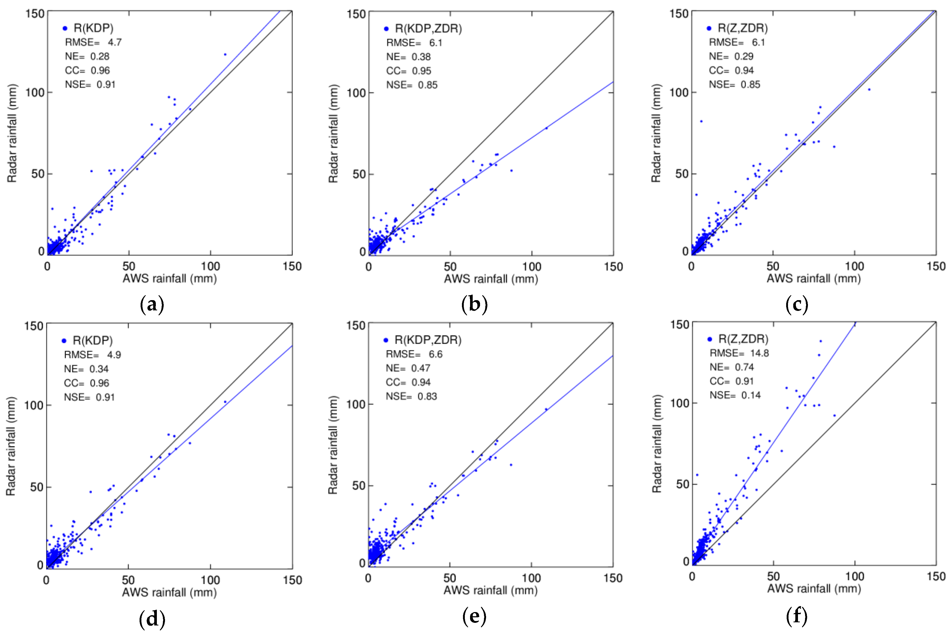
The RMSEs of R(K_DP), R(K_DP,Z_DR), and R(Z,Z_DR) with classification were 4.7 mm h⁻¹, 6.1 mm h⁻¹, and 6.1 mm h⁻¹, respectively. The corresponding values without classification were 4.9 mm h⁻¹, 6.6 mm h⁻¹, and 14.8 mm h⁻¹. The best statistical scores of all relations were obtained from R(K_DP) with classification, while the greatest improvement due to the classification was obtained with R(Z,Z_DR) (Figure 10). The statistics of another two events are summarized in

Table 7. The statistical values of each rainfall relation for all rainfall events.

Cases	Statistics	R(KDP)		R(Z,ZDR)		R(KDP,ZDR)
		Class	All	Class	All	Class	All
2011.7.9	RMSE	6.20	5.60	4.80	8.00	5.70	6.10
	NE	0.46	0.45	0.35	0.65	0.44	0.51
	CC	0.74	0.76	0.83	0.83	0.76	0.76
	NSE	0.47	0.57	0.68	0.12	0.56	0.49
2012.8.23	RMSE	3.00	3.40	3.80	8.20	3.60	4.80
	NE	0.52	0.65	0.74	1.47	0.70	0.97
	CC	0.64	0.61	0.89	0.89	0.54	0.52
	NSE	0.39	0.23	0.03	−3.42	0.16	−0.53
2012.9.8	RMSE	8.10	10.5	6.90	5.80	8.00	12.2
	NE	0.46	0.56	0.41	0.34	0.47	0.65
	CC	0.80	0.71	0.85	0.85	0.71	0.61
	NSE	0.45	0.08	0.59	0.72	0.46	−0.25
2014.8.25	RMSE	4.70	4.90	6.10	14.8	6.10	6.60
	NE	0.28	0.34	0.29	0.74	0.38	0.47
	CC	0.96	0.96	0.94	0.91	0.95	0.94
	NSE	0.91	0.91	0.85	0.14	0.85	0.83

.

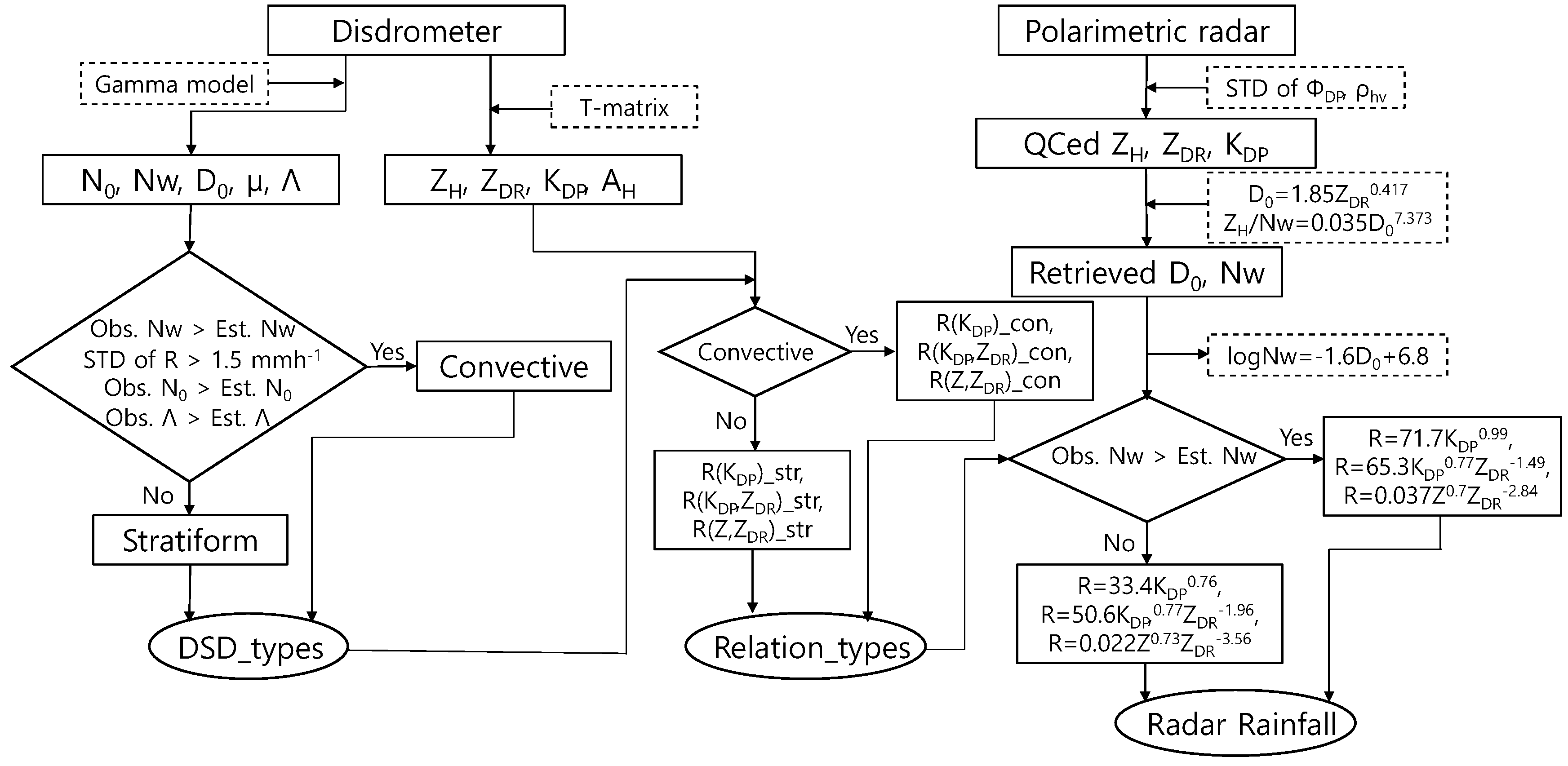
The rainfall estimation using the relations obtained from classification were better than those obtained without classification. The R(K_DP,Z_DR) with classification estimated rainfall more accurately for all rainfall events. The most improved rainfall estimation due to the classification was obtained from R(Z,Z_DR). The procedures of rainfall estimation including classification of the rainfall types from a polarimetric radar and a disdrometer are summarized in Figure 11.

4. Summary and Conclusions

To investigate the impact of rainfall type on the rainfall estimation of polarimetric variables, rainfall relations such as R(K_DP), R(K_DP,Z_DR), and R(Z,Z_DR) with respect to the precipitation type were calculated from DSDs as measured by a POSS disdrometer. The classification of rainfall type was examined by four different methods: BR03, and the logN₀–R, logNw–D₀, and Λ–R relations. The logN₀–R relation discriminated between convective and stratiform rain with less Z and Z_DR standard deviation with respect to rainfall types. The transition from convective to stratiform and vice versa occurred in the stratiform rain region for all methods. To classify the rainfall type in preparation for radar rainfall estimation, logNw and D₀ retrieved from radar polarimetric variables were used. This classification method is different from the reflectivity texture-based method that classifies more rain as convective. The performance of the DSD-based method was consistent with the vertical profile of reflectivity from a single polarimetric radar extracted at the position of two gage sites.

Statistical analysis using RMSE, NE, and CC for four different rainfall events demonstrated better rainfall estimation using the relations with precipitation types than those obtained without classification. This is not true for all the cases, however, because correct rainfall relations were not determined for transitioning rainfall and misclassified radar data. However, the R(K_DP,Z_DR) with classification performed better at estimating rainfall for all rainfall events. The greatest improvement in rainfall estimation due to the classification was obtained from R(Z,Z_DR). This may be related to the high sensitivity to drop size distribution of Z_DR with precipitation type.

As a result, we conclude that the classification of rainfall into stratiform and convective types can give more accurate rainfall estimation using polarimetric radar than without considering precipitation types in the case of R(K_DP), R(K_DP,Z_DR), and R(Z,Z_DR) in Korea, although further study using more events is needed. We also note that the rainfall types in the transition from convective to stratiform and vice versa need to be classified correctly in order to calculate rainfall from radar more accurately.

References

- Houze, R.A. Stratiform precipitation in regions of convection: A meteorological paradox? Bull. Am. Meteorol. Soc. 1997, 78, 2179–2196. [Google Scholar] [CrossRef]
- Austin, P.M.; Houze, R.A. Analysis of the structure of precipitation patterns in New England. J. Appl. Meteorol. 1972, 11, 926–935. [Google Scholar] [CrossRef] [Green Version]
- Balsley, B.B.; Ecklund, W.L.; Cater, D.A.; Riddle, A.C.; Gage, K.S. Average vertical motions in the tropical atmosphere observed by a radar wind profiler on Pohnpei (7oN lat, 157oE lon). J. Atmos. Sci. 1988, 45, 396–405. [Google Scholar] [CrossRef]
- Johnson, R.H.; Hamilton, P.J. The relationship of surface features to the precipitation and air flow structure of an intense midlatitude squall line. Mon. Weather Rev. 1988, 116, 1444–1472. [Google Scholar] [CrossRef] [Green Version]
- Bringi, V.N.; Chandrasekar, V.; Hubbert, J.; Gorgucci, E.; Randeu, W.L.; Schoenhuber, M. Raindrop size distribution in different climatic regimes from disdrometer and dual-polarized radar analysis. J. Atmos. Sci. 2003, 60, 354–365. [Google Scholar] [CrossRef]
- Marzano, F.S.; Cimini, D.; Montopoli, M. Investigating precipitation microphysics using ground-based microwave remote sensors and disdrometer data. Atmos. Res. 2010, 97, 583–600. [Google Scholar] [CrossRef]
- Leinonen, J.; Moisseev, D.; Leskinen, M.; Petersen, W.A. A climatology of disdrometer measurements of rainfall in Finland over five years with implications for global radar observations. J. Appl. Meteorol. Clim. 2012, 51, 392–404. [Google Scholar] [CrossRef] [Green Version]
- Tang, Q.; Xiao, H.; Guo, C.; Feng, L. Characteristics of the raindrop size distributions and their retrieved polarimetric radar parameters in northern and southern China. Atmos. Res. 2014, 135–136, 59–75. [Google Scholar] [CrossRef]
- Suh, S.-H.; You, C.-H.; Lee, D.-I. Climatological characteristics of raindrop size distributions in Busan, Republic of Korea. Hydrol. Earth Syst. Sci. 2016, 20, 193–207. [Google Scholar] [CrossRef] [Green Version]
- Tokay, A.; Short, D. Evidence from tropical raindrop spectra of the origin of rain from stratiform versus convective clouds. J. Appl. Meteorol. 1996, 35, 355–371. [Google Scholar] [CrossRef] [Green Version]
- Caracciolo, C.; Prodi, F.; Battaglia, A.; Porcu, F. Analysis of the moments and parameters of a gamma DSD to infer precipitation properties: A convective startiform discrimination algorithm. Atmos. Res. 2006, 80, 165–186. [Google Scholar] [CrossRef]
- Caracciolo, C.; Porcu, F.; Prodi, F. Precipitation classification at mid-latitudes in terms of drop size distribution parameters. Adv. Geosci. 2008, 16, 11–17. [Google Scholar] [CrossRef] [Green Version]
- Alvear, O.J.; Celleri, R.; Rollenbeck, R.; Bendix, J. Analysis of rain types and their Z-R relationships at different locations in the high Andes of southern Ecuador. J. Appl. Meteorol. 2017, 56, 3065–3080. [Google Scholar] [CrossRef]
- Alvear, O.J.; Celleri, R.; Rollenbeck, R.; Bendix, J. Optimization of X-band radar rainfall retrieval in the southern Andes of Ecuador using a random forest model. Remote Sens. 2019, 11, 1632. [Google Scholar] [CrossRef] [Green Version]
- Rollenbeck, R.; Bendix, J. Rainfall distribution in the Andes of southern Ecuador derived from blending weather radar data and meteorological field observations. Atmos. Res. 2011, 99, 277–289. [Google Scholar] [CrossRef]
- Bringi, V.N.; Williams, C.R.; Thurai, M.; May, P.T. Using dual-polarized radar and dual-frequency profiler for DSD characterization: A case study from Darwin, Australia. J. Atmos. Ocean. Technol. 2009, 26, 2107–2122. [Google Scholar] [CrossRef]
- Penide, G.; Kumar, V.V.; Protat, A.; May, P.T. Statistics of drop size distribution parameters and rain rates for stratiform and convective precipitation during the north Australian wet season. Mon. Weather Rev. 2013, 141, 3222–3237. [Google Scholar] [CrossRef]
- Steiner, M.; Houze, R.A.; Yuter, S.E. Climatological characterization of three-dimensional storm structure from radar and rain gauge data. J. Appl. Meteorol. 1995, 34, 1978–2007. [Google Scholar] [CrossRef]
- Steiner, M.; Houze, R.A. Three-dimensional validation at TRMM ground truth sites: Some early results from Darwin, Australia. In Proceedings of the 26th Conference on Radar Meteorology, Norman, OK, USA, 24–28 May 1993; pp. 417–420. [Google Scholar]
- Penide, G.; Protat, A.; Kumar, V.V.; May, P.T. Comparison of two convective/stratiform precipitation classification techniques: Radar reflectivity texture versus drop size distribution-based approach. J. Atmos. Ocean. Technol. 2013, 30, 2788–2797. [Google Scholar] [CrossRef]
- Thompson, E.J.; Rutledge, S.A.; Dolan, B.; Thurai, M. Drop size distributions and radar observations of convective and stratiform rain over the Equatorial Indian and west Pacific oceans. J. Atmos. Sci. 2015, 72, 4091–4125. [Google Scholar] [CrossRef]
- You, C.-H.; Lee, D.-I.; Kang, M.-Y.; Kim, H.-J. Classification of rain types using drop size distributions and polarimetric radar: Case study of a 2014 flooding event in Korea. Atmos. Res. 2016, 181, 211–219. [Google Scholar] [CrossRef]
- Ryzhkov, A.V.; Zrnic, D.S. Assessment of rainfall measurement that uses specific differential phase. J. Appl. Meteorol. 1996, 35, 2080–2090. [Google Scholar] [CrossRef]
- May, P.; Keenan, T.D.; Zrnic, D.S.; Carey, L.; Rutledge, S. Polarimetric radar measurement of tropical rain at 5-cm wavelength. J. Appl. Meteorol. 1999, 38, 750–765. [Google Scholar] [CrossRef]
- Bringi, V.N.; Chandrasekar, V. The Polarimetric Basis for Characterizing Precipitation. Polarimetric Doppler Weather Radar: Principles and Applications; Cambridge University Press: Cambridge, UK, 2001; pp. 378–533. [Google Scholar]
- Ryzhkov, A.V.; Schuur, T.J.; Burgess, D.W.; Heinselman, P.L.; Giangrande, S.E.; Zrnic, D.S. The Joint Polarization Experiment: Polarimetric rainfall measurements and hydrometeor classification. Bull. Am. Meteorol. Soc. 2005, 86, 809–824. [Google Scholar] [CrossRef] [Green Version]
- Cifelli, E.V.; Chandrasekar, V.; Lim, S.; Kennedy, P.C.; Wang, Y.; Rutledge, S.A. A new dual-polarization radar rainfall algorithm: Application in Colorado precipitation events. J. Atmos. Ocean. Technol. 2011, 28, 352–364. [Google Scholar] [CrossRef] [Green Version]
- Ryzhkov, A.; Dieberich, M.; Zhang, P.; Simmer, C. Potential utilization of specific attenuation for rainfall estimation, mitigation of partial beam blockage, and radar networking. J. Atmos. Ocean. Technol. 2014, 31, 599–619. [Google Scholar] [CrossRef]
- You, C.-H.; Kang, M.-Y.; Lee, D.-I.; Uyeda, H. Rainfall estimation by S-band polarimetric radar. Part I: preprocessing and preliminary results. Meteorol. Appl. 2014, 21, 975–983. [Google Scholar]
- Sheppard, B.E. Measurement of raindrop size distributions using a small Doppler radar. J. Atmos. Ocean. Technol. 1990, 7, 255–268. [Google Scholar] [CrossRef] [Green Version]
- You, C.-H.; Lee, D.-I.; Kang, M.-Y. Rainfall estimation using specific differential phase for the first operational polarimetric radar in Korea. Adv. Meteorol. 2014, 2014, 41317. [Google Scholar] [CrossRef] [Green Version]
- You, C.-H.; Lee, D.-I. Algorithm development of the optimum rainfall estimation using polarimetric variables in Korea. Adv. Meteorol. 2015, 2015, 395937. [Google Scholar] [CrossRef]
- Adirosi, E.; Roberto, N.; Montopoli, M.; Gorgucci, E.; Baldini, L. Influence of disdrometer type on weather radar algorithms from measured DSD: Application to Italian climatology. Atmosphere 2018, 9, 360. [Google Scholar] [CrossRef] [Green Version]
- Matrosov, Y.S.; Ciffelli, R.; Neiman, J.P.; White, B.A. Radar rain-rate estimators and their variability due to rainfall type: An assessment based on hydrometeorology testbed data from the southeastern United States. J. Appl. Meteorol. 2016, 55, 1345–1358. [Google Scholar] [CrossRef]
- You, C.-H.; Lee, D.-I. Decadal variation in raindrop size distributions in Busan, Korea. Adv. Meteorol. 2015, 2015. [Google Scholar] [CrossRef]
- Waterman, P.C. Symmetry, unitarity, and geometry in electromagnetic scattering. Phys. Rev. 1971, D3, 825–839. [Google Scholar] [CrossRef]
- Mishchenko, M.I.; Travis, L.D.; Mackowski, D.W. T-matrix computations of light scattering by nonspherical particles: A review. J. Quant. Spectrosc. Radiat. Transf. 1996, 55, 535–575. [Google Scholar] [CrossRef]
- Beard, K.V.; Chuang, C. A new model for the equilibrium shape of raindrops. J. Atmos. Sci. 1987, 44, 1509–1524. [Google Scholar] [CrossRef]
- Andsager, K.; Beard, K.V.; Laird, N.S. A laboratory study of oscillations and axis ratios for large raindrops. J. Atmos. Sci. 1999, 55, 208–226. [Google Scholar]
- Huang, G.-J.; Bringi, V.N.; Thurai, M. Orientation angle distributions of drops after 80 m fall using a 2D-video disdrometer. J. Atmos. Ocean. Technol. 2008, 25, 1717–1723. [Google Scholar] [CrossRef]
- Atlas, D.; Srivastava, R.; Sekhon, R.S. Doppler radar characteristics of precipitation at vertical incidence. Rev. Geophys. 1973, 11, 1–35. [Google Scholar] [CrossRef]
- Ulbrich, C.W. Natural variations in the analytical form of the raindrop size distribution. J. Appl. Meteorol. Clim. 1983, 22, 1764–1775. [Google Scholar] [CrossRef] [Green Version]
- Zhang, G.; Vivekanandan, J.; Brandes, E.; Menegini, R.; Kozu, T. The shape-slope relation in observed gamma raindrop size distributions: Statistical error or useful information? J. Atmos. Ocean. Technol. 2003, 20, 1106–1119. [Google Scholar] [CrossRef] [Green Version]
- Testud, J.; Oury, S.; Black, R.; Amayenc, P.; Dou, X. The concept of ‘‘normalized’’ distribution to describe raindrop spectra: A tool for cloud physics and cloud remote sensing. J. Appl. Meteorol. 2001, 40, 1118–1140. [Google Scholar] [CrossRef]
Figure 1.
The location of Bislsan (BSL) radar (full rectangle), the Precipitation Occurrence Sensor System (POSS) disdrometer (open rectangle), and the rain gages (plus). The Bislsan radar is located at the center of the right panel, and concentric circles are drawn around it with radii at 50 km intervals. The cross with plus symbols show the gate sites used for calculating total rainfall amount and open diamond with plus is the gage site for verifying the classification performance.
Figure 2.
The cumulative occurrence plot of ZH and ZDR for classified as stratiform rainfall, as calculated from rainfall rate temporal variability (a) BR03, (b) logN0-R relation, (c) logNw-D0 relation, and (d) Λ-R relation. The bin size of ZH and ZDR is 1 dBZ and 0.1 dB.
Figure 3.
The cumulative occurrence plot of ZH and ZDR for classified as convective rainfall, as calculated from rainfall rate temporal variability (a) BR03, (b) logN0-R relation, (c) logNw-D0 relation, and (d) Λ-R relation. The bin size of ZH and ZDR is 1 dBZ and 0.1 dB.
Figure 4.
The plan position indicator of (a) ZH and (b) ΦDP at an elevation angle of 0.5° on 03:00 LST 8 September 2012 and (c) ZH and (d) ΦDP on 13:00 LST 25 August 2015.
Figure 5.
The classification of precipitation types using (a,c) DSD-based and (b,d) SHY method on 03:00 LST 8 September 2012 and 13:00 LST 25 August 2014, respectively. The blue (red) color shows the regions classified as a stratiform (convective).
Figure 6.
The vertical profile of reflectivity extracted from Gudeoksan radar at gage site (a) ID 162 on 23 August in 2012 and (b) ID 926 on 25 August in 2014. The asterisk (open circle) on the image shows the classified as a convective (stratiform) rain from the retrieved DSDs at the gage site.
Figure 7.
The highest hourly and accumulated rainfall amounts recorded at (a) Geumcheon (ID 848) on 9 July 2011, (b) Daebyung (ID 945) on 23 August 2012, (c) North Changwon (ID 255) on 8 September 2012, and (d) Geumjeong (ID 939) on 25 August 2014. Left (right) axes and grey filled bars (red lines) show hourly (accumulated) rainfall amount (mm).
Figure 8.
The spatial distribution of accumulated rainfall amounts recorded at rain gages within radar coverage (a) on 9 July 2011, (b) on 23 August 2012, (c) on 8 September 2012, and (d) on 25 August 2014.
Figure 9.
Scatter plots of hourly gage rainfall against rainfall amounts obtained from the radar rainfall relationships (a,d) R(KDP), (b,e) R(KDP,ZDR), (c,f) R(Z,ZDR) with and without classification on 23 August 2012, respectively. Nash–Sutcliffe efficiency (NSE).
Figure 10.
Scatter plots of hourly gage rainfall against rainfall amounts obtained from the radar rainfall relationships (a) R(KDP), (b) R(KDP,ZDR), (c) R(Z,ZDR) with classification, (d) R(KDP), (e) R(KDP,ZDR), and (f) R(Z,ZDR) on 25 August 2014 without classification, respectively.
Figure 11.
The flowchart of rainfall estimation through calculation of rainfall relation with respect to the rainfall types.