Convective Shower Characteristics Simulated with the Convection-Permitting Climate Model COSMO-CLM


1
Institute for Atmospheric and Environmental Sciences, Goethe University Frankfurt, 60438 Frankfurt, Germany
2
Centre National de Recherches Météorologiques, 31100 Toulouse, France
*
Author to whom correspondence should be addressed.
Atmosphere 2019, 10(12), 810; https://doi.org/10.3390/atmos10120810
Submission received: 24 October 2019
/
Revised: 9 December 2019
/
Accepted: 11 December 2019
/
Published: 13 December 2019
(This article belongs to the Section Meteorology)
Abstract
:This paper evaluates convective precipitation as simulated by the convection-permitting climate model (CPM) Consortium for Small-Scale Modeling in climate mode (COSMO-CLM) (with 2.8 km grid-spacing) over Germany in the period 2001–2015. Characteristics of simulated convective precipitation objects like lifetime, area, mean intensity, and total precipitation are compared to characteristics observed by weather radar. For this purpose, a tracking algorithm was applied to simulated and observed precipitation with 5-min temporal resolution. The total amount of convective precipitation is well simulated, with a small overestimation of 2%. However, the simulation underestimates convective activity, represented by the number of convective objects, by 33%. This underestimation is especially pronounced in the lowlands of Northern Germany, whereas the simulation matches observations well in the mountainous areas of Southern Germany. The underestimation of activity is compensated by an overestimation of the simulated lifetime of convective objects. The observed mean intensity, maximum intensity, and area of precipitation objects increase with their lifetime showing the spectrum of convective storms ranging from short-living single-cell storms to long-living organized convection like supercells or squall lines. The CPM is capable of reproducing the lifetime dependence of these characteristics but shows a weaker increase in mean intensity with lifetime resulting in an especially pronounced underestimation (up to 25%) of mean precipitation intensity of long-living, extreme events. This limitation of the CPM is not identifiable by classical evaluation techniques using rain gauges. The simulation can reproduce the general increase of the highest percentiles of cell area, total precipitation, and mean intensity with temperature but fails to reproduce the increase of lifetime. The scaling rates of mean intensity and total precipitation resemble observed rates only in parts of the temperature range. The results suggest that the evaluation of coarse-grained (e.g., hourly) precipitation fields is insufficient for revealing challenges in convection-permitting simulations.
1. Introduction
The correct representation of deep convection in climate models is essential for assessing the risks associated with this phenomenon like wind gusts, hail, lightning, and flash floods. Convection-permitting climate models (CPMs) that simulate deep convection explicitly improve the representation of the diurnal cycle of precipitation and the simulation of extreme precipitation intensities on short time scales compared to models that parameterize convection [1,2,3,4]. The vast majority of studies evaluating precipitation in CPMs use rain gauge data or gridded precipitation data sets based on gauge data as observations. However, this traditional evaluation of precipitation has limitations for evaluating convective precipitation since the typical dimension of convective storms is smaller than the distance between stations. This can lead to an underestimation of storm frequency and storm peak intensity [5]. An evaluation of the space-time dynamics of convective cells requires the finer spatial and temporal resolution of remote sensing techniques. Since the temporal and spatial resolution of radar data is finer than the characteristic scales of convective clouds, it allows for continuous tracking of convective cells over their life cycle. Although mainly used for now-casting purposes, tracking of radar data to derive characteristics of convective cells on climatological time scales has been done in a few studies, for example, [6,7]. Precipitation output of convection-permitting climate models has rarely been used for tracking so far. Brisson et al. [8] simulated selected days of high convective activity and compared the life cycle of precipitation intensity of convective cells to radar data. Prein et al. [9] conducted a comparison of hourly precipitation from a CPM and radar data in order to evaluate the model’s capability to simulate mesoscale convective systems in North America. To the authors’ knowledge, sub-hourly precipitation output from continuous CPM simulation has not been evaluated yet. This is why we apply a tracking algorithm to 5-min precipitation output of a CPM and to a newly developed 5-min precipitation climatology based on gauge adjusted radar data. The first aim of this study is to evaluate the characteristics of convective precipitation objects (the term convective cells is used synonymously from now on) in a CPM in terms of lifetime, mean precipitation intensity, area, and total precipitation.
Because of climate change, the hydrological cycle is expected to intensify with increasing temperatures, leading to changes in intensity, frequency, and duration of precipitation events [10]. The question of how the characteristics of deep convection and the accompanying extreme short-term precipitation events will change is still being discussed. Observational studies [11,12] have reported intensification of hourly precipitation above the Clausius–Clapeyron rate (the increase of the saturation water vapor pressure with temperature) of ca. 7%/K. Different hypotheses have been suggested to explain this behavior, for example, the invigoration of convective cells through a positive feedback loop caused by increased moisture availability at higher temperatures leading to increased latent heat release in the updraft of convective cells, which, in turn, leads to higher updraft speeds and increased moisture convergence at the cloud base [13]. Moseley et al. [7] investigated the life cycle of convective precipitation cells by tracking radar data. They showed a stronger increase in mean intensity of convective precipitation cells with temperature than for stratiform cells. The application of a tracking algorithm allows us to investigate the temperature dependence of cell characteristics. Therefore, the second aim of this study is to gain insights into how well the model can reproduce the temperature scaling of cell characteristics observed in the radar data.
The paper is structured as follows: In the following section, the model setup and the radar data will be introduced, followed by a description of the cell tracking algorithm. The subsequent result section starts with an evaluation of stationary precipitation statistics. Afterward, the characteristics and spatial distribution of convective cells in the convection-permitting simulation are compared to the radar data. The section is concluded by the investigation of the temperature dependence of the cell characteristics. In the final section, the results are summarized, and conclusions are drawn.
2. Data and Methods
2.1. Model Setup
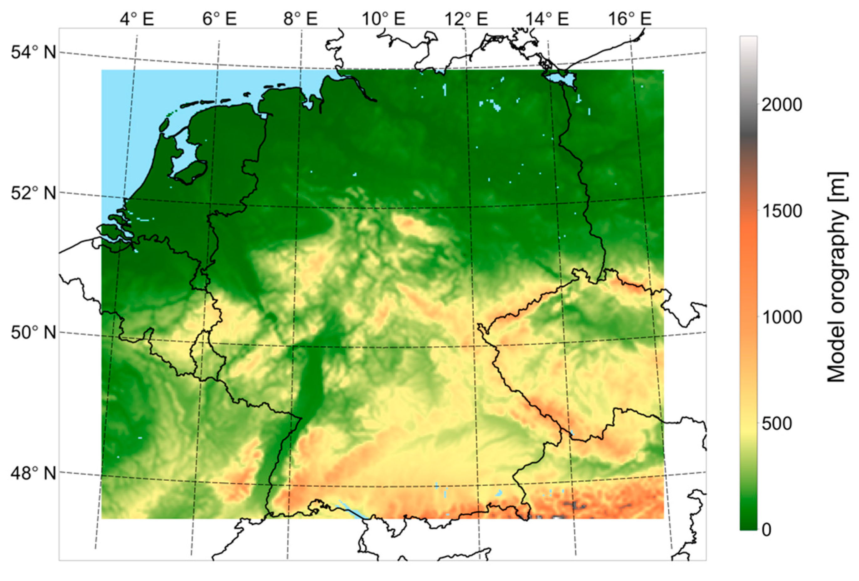
The Consortium for Small-Scale Modeling model in climate mode (COSMO-CLM, from now on abbreviated as CCLM) is used to downscale the European Centre for Medium-Range Weather Forecast Interim Reanalysis (ERA-Interim) to a horizontal grid spacing of 0.025° (≈2.8 km) via an intermediate nest with a grid spacing of 0.22° (≈25 km). At the lateral boundaries of the simulation domain, the model is nudged towards the driving data using Davies relaxation [14]. Within the simulation domain, no nudging is applied. The model domain of the inner nest covers central Europe (Figure 1). The CCLM is a non-hydrostatic limited-area climate model based on the COSMO model [15], a model designed by the Deutsche Wetterdienst (DWD) for operational weather predictions. The climate limited-area modeling (CLM) community adapted this model to perform climate projections [16,17]. We use the version COSMO5.0clm7 with the following setup. For time integration, the 5th order Runge–Kutta split-explicit time-stepping scheme is used with a time step of 25 s. The lower boundary fluxes are provided by the TERRA model. The radiative scheme is the Ritter and Geleyn scheme [18] and is called every 15 min. As recommended in Brisson et al. [19], we use a one-moment microphysics scheme, including graupel in the finest nest, which provides a more realistic representation of deep convective clouds. While the parameterization of deep convection is switched off, shallow convection is still parameterized using the convection scheme after Tiedtke et al. [20]. The simulation covers the period from 1983 to 2015. Surface temperature and precipitation output are stored every 5 min. Since the evaluation data set is available from 2001, the evaluation period is 2001–2015.
2.2. Radar Data
As a reference for the model evaluation, we use the radar-based precipitation climatology developed by DWD [21]. This precipitation data set is based on radar data that has been quality checked and adjusted to rain gauge measurements. The correction steps used for this product to derive precipitation from radar reflectivity include clutter filtering, distance-dependent signal correction, and removal of radar spokes. For the tracking, we use the 5-min dataset (YW-product) [22]. For the comparison of mean precipitation and for the comparison of stationary hourly precipitation intensities, we use the hourly dataset (RW-product) [23]. The full data set covers the time period 2001–2018. The data set has a spatial grid resolution of 1 km × 1 km. For the evaluation, the radar data is conservatively remapped to 2.8 km × 2.8 km. In order to assess the impacts of this remapping on the tracking results, the results of tracking the data in the original resolution are often shown in addition.
2.3. Tracking Algorithm
To obtain the characteristics of convective objects from model and radar data, we use a tracking algorithm. The tracking consists of three major steps:
- Contiguous precipitation areas with precipitation intensity above a threshold of 8.5 mm/h (within 5 min), potential convective objects, are identified in the current and the subsequent time step. Contiguous areas are defined as pixels that share a common edge.
- Wind information is used to predict the position of the object at the subsequent time step. To this end, a “cone of detection” is set up for each pixel of every object, and the cone is swept for precipitation objects from the subsequent time step. The axis of the cone is defined by the wind direction; the length of the cone is calculated as twice the wind speed. The opening angle of the cone is 45°. If a new cell is present in the cone, a probability value is assigned to the origin pixel of the cone, which links this pixel to the new cell. The probability value is highest in the center of the cone and drops off exponentially in all directions. As an example, Figure 2a shows the probability values for a single pixel in the case of purely westward wind. In this case, the probability is calculated according to the following formula:where x and y are the indices in x and y direction starting at the original pixel (0,0). The parameter Ycent denotes the centerline of the cone, and Xmax is the length of the cone, as determined by the wind data. This procedure is repeated for wind information in three height levels (500, 700, and 850 hPa). Afterward, the height dependent probability values are averaged to obtain the final probability value.
- In the next step, the probabilities of all pixels are summed up for each cell. If one single object is present in the cone, the corresponding objects from the current and the subsequent time step are connected. If multiple cells are present, the current cell is associated with the cell with the highest probability in the subsequent time step.
The characteristics that are extracted by the algorithm are cell lifetime, mean intensity, maximum intensity, area, cell speed, and track length. It should be noted that merges and splits of objects are not accounted for. If two cells merge, the cell track with the higher probability of association is continued, whereas the other track ends. The track that is not continued is regarded as an individual track in itself. Figure 2b shows an example of a tracked precipitation object.
Only cells with a lifetime of at least three time steps (=15 min) are considered for analysis. This condition reduces the chances of misinterpreting single clutter pixels in the radar data (which are still present but heavily reduced compared to operational radar products) as convective cells. Furthermore, the algorithm only selects precipitation areas larger than four grid boxes for the same reason. For consistency, this requirement is also kept when tracking the model data. This requirement is also justified because the effective resolution of any numerical model is always coarser than the grid spacing. When applying the tracking algorithm to the model data, the model data is conservatively remapped to the polar stereographic projection of the radar data in order to have both data sets on a common, equidistant grid for ease of comparison. The wind information used for estimating the position of each cell at the subsequent time step is taken from the ERA-Interim reanalysis in case of the radar data. In the case of the simulation data, the wind information from the intermediate nest driving the finer simulation is used.
3. Results and Discussion
3.1. Precipitation Statistics
We first evaluate the mean precipitation sum in the simulation with respect to the radar climatology on the common 2.8-km grid. The highest precipitation amount is found in the Alps (Figure 3). Least precipitation occurs in the North-East of Germany. The mean daily precipitation in observation and simulation data is 2.0 mm/d and 1.7 mm/d, respectively, resulting in a 14% underestimation of total precipitation in the simulation. Considering that no bias correction [24] has been applied, this is in line with other CPM evaluations. The model overestimates precipitation in mountainous regions, especially in the Black Forest in southwest Germany, and underestimates it in the lowlands of Northern Germany. This points to an overestimation of the orographic intensification of precipitation in the simulations. Unfortunately, no measurement uncertainty is provided for the radar data. Since other gridded precipitation data sets also show considerable deviations from each other [25], a detailed comparison of the radar data set to other precipitation data would be beneficial. In a first comparison to a daily gridded observational dataset for precipitation, temperature, and sea level pressure in Europe (E-OBS, version 20.e, [26]), we find that areal mean precipitation in the radar data is 5.9% smaller than in E-OBS. This is in line with Winterrath et al. [21], who compared the radar data to a station-based data set and found the precipitation amount in the radar data to be smaller, especially in mountain areas. The spatial pattern of underestimation in the North and overestimation in the mountains is also present when comparing the simulation to the E-OBS data set (not shown).
We restrict our analysis of convective cells to the summer half-year from April to September because convective precipitation mainly occurs in this period. The mean observed and simulated summer precipitation (April to September) is 2.3 mm/d and 1.5 mm/h, respectively, resulting in an underestimation of 34% in the simulation. Taking into account that convective precipitation occurs almost exclusively in the summer months in Germany, this indicates that the model underestimates convective precipitation more than stratiform precipitation. The underestimation is strongest in Northern Germany, while more realistic precipitation amounts are simulated in the South.
The simulated probability distribution of hourly precipitation compares well with the observed one (Figure 4). The observed wet hour frequency defined as hours with precipitation above 0.1 mm/h is 8.5 %; the simulated wet hour frequency is 9.6%. The Perkin’s Skill Score (PSS), which calculates the overlapping area between observed and modeled probability distribution function [27], is 0.89 for the wet hour frequency. The simulation considerably underestimates precipitation occurrence in the range below 12 mm/h. This range contributes 95% to the total observed precipitation sum and is underestimated by ca. 28%. The precipitation sum resulting from intensities between 12 mm/h and 50 mm/h is overestimated by 12%. The occurrence of hourly precipitation sums above 50 mm/h is underestimated by 32%. Considering the 5-min intensity distribution, the model always underestimates precipitation intensity. The drop-off at the highest 5-min intensities corresponds well with the drop-off at the hourly time scale. However, the fact that there is no overestimation of high intensities corresponding to the one at the hourly time scale points to differences in the dynamics of convective cells.
3.2. Frequency and Characteristics of Convective Cells
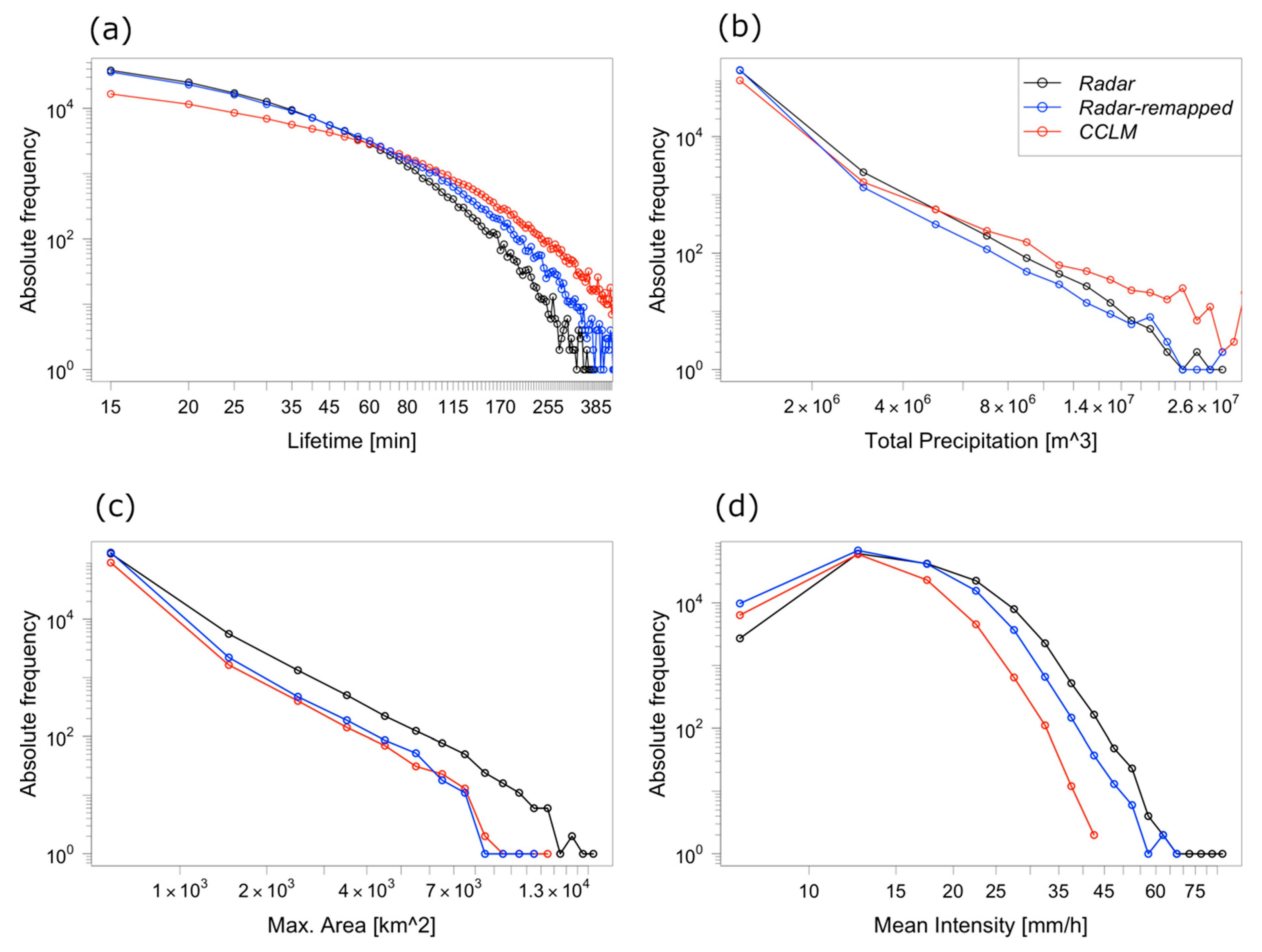
In this subsection, we compare the simulated frequency distributions of cell characteristics with the radar characteristics. The simulation underestimates convective activity, represented by the total number of convective cells, by 33%. Convective precipitation, calculated as the precipitation sum of all convective cells, is very well matched with an overestimation of 2%. The lifetime of convective cells ranges from 15 min (the lowest possible value as set by the tracking algorithm) to 7 h (Figure 5). As expected, short-living cells are the most common form of convective cells. The simulation captures but underestimates the decrease in frequency with lifetime and produces too many long-living and too few short-living cells. Comparing the lifetime distributions of the simulation and remapped radar data yields a PSS of 0.84. A possible reason for the overestimation of cell lifetime could be that tracks are more often lost in the radar data than in the simulation data by the tracking algorithm. The reason for this is that radar data provide snapshots of precipitation, whereas, in the model, precipitation is accumulated, which leads to a smoother precipitation field. This difference of accumulated versus instantaneous precipitation also has a small influence on cell size and mean intensity. To estimate how many tracks are wrongfully split up by the tracking algorithm, we investigate the cell size at the first occurrence of the cell. If the cell only just started its life cycle, one would expect a small size close to the lower boundary of five grid points. If, on the other hand, the cell is the second part of a track that was wrongfully split up, it will have a larger extent. If we consider an initial area larger than 10 grid points (80 km2) to be unrealistically large and discard those cells, then the underestimation of convective activity is only slightly reduced to 28%.
The frequency distributions of cell area and total precipitation per cell are very well matched with a PSS of 0.99 and 0.98, respectively. There are too few high-intensity cells. The PSS for the mean intensity is 0.86.
To verify that it is really the long-living convective cells that have a high intensity and area, Figure 6 shows the distributions of mean intensity and of maximum area depending on the lifetime of the convective cells. To this end, cells are grouped into lifetime classes of 15-min width. A systematic increase in maximum area and mean intensity with lifetime can be seen in both the radar observations and the simulation. While the observed median maximum area is 226 km2 for cells living 195 to 210 min, the median is only 25 km2 for cells living 15 to 30 min. The observed median values of mean intensity of cells in the same lifetime classes are 21 mm/h for long-living and 12 mm/h for short-living cells. These relationships indicate that the detected short-living cells can either be single-cell storms or individual cells of a multicell storm. The long-living, large, and intense cells are organized forms of convective systems like squall lines, supercells, and mesoscale convective systems. The simulation systematically underestimates the increase in mean intensity with lifetime. The increase in maximum area is well matched.
3.3. Spatial Distribution of Cell Characteristics
Figure 7 shows the spatial distribution of the occurrence of convective cells. Here, the occurrence of convective cells per grid-point for the period 2001–2015 is shown. The tracking algorithm stores the area and center of mass for each cell at every point in time. For this reason, no information about the actual shape of a cell is available. Instead, the cells are reconstructed as squares around the center of mass to match their original size. It has to be noted that every occurrence of a cell per 5-minute time step is counted. The value can, thus, be interpreted as the number of exceedances of a 5-minute precipitation intensity of 8.5 mm/h (the detection threshold of the tracking algorithm). Instead of counting each cell only once (e.g., at its point of largest extent), this method represents the area affected by convective cells more realistically because cells can have widely varying areas and translation speeds.
Mountain ranges facilitate the triggering of deep convection through various processes (see Kirshbaum et al. [28] for a review). Therefore, it is not surprising that the Alps and the pre-alpine region show the highest occurrence of convective cells. Low mountain ranges also show increased values compared to lowland regions. The overall pattern matches the climatology of convective activity derived from lightning data presented in Wapler [29]. In general, there is a positive North–South gradient in convective activity. The mean intensity of convective cells is lower over the mountains (not shown). This can be explained by the fact that orographically induced convection is early in its life cycle in this area and, thus, has a relatively low intensity.
In general, the simulation is capable of representing the increased convective activity in mountain areas. It overestimates the number of convective cells in the South and underestimates it in the North (Figure 7). However, there are areas of overestimation and underestimation in both parts of the investigated domain. Near the radar locations, overestimation prevails, while areas of underestimation tend to be located furthest away from the radar. More cells are initiated in the mountainous areas of Southern Germany than in the North. This supports the hypothesis that the more complex topography facilitates the onset of convection and, thus, eliminates the negative bias in the cell number present in Northern Germany.
Since the convective activity shows a different pattern in North and South Germany, which may be related to the different orography in these regions, we further investigate the height dependence of convective activity. Therefore, the convective cells are stratified by the terrain height at which they occur. While the cell number is underestimated by 15% in regions with a terrain height below 400 m a.s.l., the number of cells for terrain heights above 400 m a.s.l. is overestimated by 6%. The overestimation of convective precipitation in mountainous areas is in line with results in Knist et al. [30], who performed convection-permitting climate simulations over Germany using the WRF-model and compared the results to gauge data.
3.4. Diurnal Cycle
The diurnal cycle of convective activity in Central Europe has a pronounced maximum in the afternoon, which is caused by daytime land surface heating [31]. The diurnal cycle of convective activity is slightly delayed in the simulation (Figure 8a). The afternoon maximum is observed at 15:50 (UTC), while the modeled maximum occurs around 16:30 (UTC). The number of cells initiated during the night and morning is well matched, whereas the daytime increase of convective activity is too small, resulting in 36% fewer cells being initiated in the afternoon and evening (between 13:00 UTC and 20:00 UTC). The maximum number of cell initiation is underestimated by 40%. Combined with the general overestimation of cell lifetime, this leads to an overestimation of cells present at each point in time during the night and an underestimation during the time of highest activity (Figure 8b). The mean intensity, defined as the mean over all cells of spatial mean intensity at every 5-min time step, increases during the daytime. The modeled increase of mean intensity is too weak.
While the peak of convective activity in areas with an elevation below 400 m is underestimated, the convective activity above 400 m is well simulated (Figure 9). The sum of convective precipitation is overestimated in mountainous areas, which is caused by an overestimation of cell size during the daytime, which is especially pronounced in the afternoon.
3.5. Temperature Scaling of Cell Characteristics
In this subsection, we investigate the temperature scaling of cell properties like total precipitation, area, and mean intensity. We assign the mean daily temperature to each cell. Mean daily temperature is chosen instead of, for example, hourly temperature, to minimize the effect of local processes like cold pool formation on the scaling rate [11,32]. For the radar data, we use ERA-Interim 2-m temperature of the grid point closest to the origin of the convective cell. For the simulation data, we use the simulated 2-m temperature at the location of cell origin directly. Afterward, we group the convective cells properties total precipitation, maximum area, and lifetime and mean intensity into temperature bins of 1 °C width and determine the 90th, 95th, and 99th percentile for each bin.
The scaling of total precipitation, mean intensity, and lifetime and maximum area for both radar and simulation data is shown in Figure 10. Shown are the aforementioned percentiles based on the simulation and the remapped radar data. For comparison, the 95th percentile of the original radar data is shown additionally. The general underestimation of the highest percentiles of the variables mean intensity and total precipitation, as well as the overestimation of lifetime, is also visible here. In contrast to these variables, the maximum area is well represented in the model both in absolute value as well as the scaling rate. Generally, the rate at which mean intensity increases with temperature is well reproduced by the model. However, the underestimation of precipitation intensity for long-lasting, organized cells shown in Section 3.2 is visible in the scaling rates of mean intensity. While the radar data shows an exponential increase up to the highest temperatures, the simulated mean intensity flattens at 20 °C. The largest difference in scaling rate appears for the lifetime of convective cells. The radar data shows an increase in lifetime of ca. 5% in the temperature range between 13 and 22 °C and flattens at higher temperatures. In contrast to this, the lifetime of convective cells in the simulation is mostly flat with small increases only in the low-temperature range and a drop at high temperatures. An intensification of convective cells above the Clausius–Clapeyron rate, which supports the hypothesis of a positive feedback loop in the strength of convective cells with rising temperatures, is apparent from the scaling rate of the total precipitation. The scaling of the modeled total precipitation is larger than the Clausius–Clapeyron rate for the whole temperature range up to 23 °C, where it levels off. This leveling off is also frequently reported for scaling of extreme precipitation at fixed locations and attributed to limited moisture supply at high temperatures [33,34]. The observed total precipitation shows a slightly different behavior with a smaller increase at low temperatures and a larger increase starting at 15 °C.
4. Conclusions
In this study, we evaluate the representation of convective precipitation objects in a CPM by applying a tracking algorithm to 5-min precipitation output and a newly developed 5-min radar climatology over Germany. The model is capable of reproducing the total amount of convective precipitation, as well as the frequency and characteristics of convective cells ranging from short-living, small cells to long-living, intense cells. However, the number of convective cells is underestimated. This underestimation is compensated by an overestimation of cell lifetime. A possible explanation for the underestimation of convective activity and the overestimation of cell lifetime could be that the grid size of 2.8 km is too coarse to capture boundary layer inhomogeneities, which facilitate the initiation of convection; thus, the number of cells is reduced. At the same time, convective available potential energy (CAPE) can accumulate longer without being consumed by convection, and the cells that manage to evolve can live longer. The observed enhanced convective activity in the mountain ranges is reproduced by the model. However, convective activity is underestimated in the lowlands of Northern Germany and overestimated in the mountainous regions of Southern Germany. This supports the hypothesis that the grid size is too coarse to fully represent the initiation of deep convection without the help of orographic forcing. However, it cannot be ruled out that other model deficiencies contribute to this bias. The difference in representing convective precipitation in mountainous areas and lowland regions agrees with an evaluation of the WRF-CPM [30]. The fact that both models overestimate convective precipitation in the mountains whilst giving correct amounts in the lowlands might indicate a general, model-independent problem, such as resolution, which is 2.8 km in both studies. The underestimation of mean intensity and maximum intensity of large, long-living cells suggests model deficiencies in representing large, organized forms of convection. To evaluate the model’s capability of representing the characteristics of extreme convective cells at different temperatures, we investigate the temperature scaling of cell characteristics. While the model can reproduce the increases in mean intensity and area of extreme convective cells with temperature, it fails to reproduce the increasing cell lifetime seen in observations. The simulated scaling of total precipitation shows a continuous increase above the Clausius–Clapeyron rate, which indicates dynamical changes in extreme convective cells with increasing temperature. The observations show different scaling rates with a value close to the Clausius–Clapeyron rate at temperatures below 15 °C and higher values above. More detailed investigations are needed to understand these differences. Further studies could investigate the scaling behavior of forced vs. unforced convection. Additionally, the combination of the tracking algorithm with spectral methods characterizing the organization of the precipitation field, for example, Brune et al. [35], could yield insight into the organization of deep convection.
The approach presented here can be used for more detailed process studies of deep convection in regional climate models, for example, focusing on different synoptical situations with potentially different types of convection, as investigated in Wapler et al. [36]. It might also be beneficial to evaluate the consequences of changing the model setup by increasing resolution or switching to a more sophisticated (i.e., two-moment) microphysics scheme. Furthermore, this study can be the basis for gaining confidence in the representation of different types of convection in order to use the output from RCMs for hydrological applications. One idea could be to construct a synthetic time series of convective precipitation objects that are derived from RCM output and bias-corrected with radar data to estimate the hydrological consequences of the projected increase in heavy precipitation events.
Author Contributions
Conceptualization, B.A., E.B., and C.P.; Methodology, E.B., and C.P.; Software, C.P. and E.B.; Formal Analysis, C.P.; Investigation, C.P. and E.B.; Resources, B.A.; Data Curation, E.B., and C.P.; Writing-Original Draft, C.P.; Writing-Review and Editing, C.P., E.B., and B.A.; Visualization, C.P.; Supervision, B.A.; Project Administration, B.A., Funding Acquisition, B.A.
Funding
This research was funded by „Hessisches Landesamt für Naturschutz, Umwelt und Geologie“ and „Rheinland-Pfalz Kompetenzzentrum für Klimawandelfolgen“, project name: “Konvektive Gefährdung über Hessen und Rheinland-Pfalz”.
Acknowledgments
We thank the „Hessisches Landesamt für Naturschutz, Umwelt und Geologie“ and the „Rheinland-Pfalz Kompetenzzentrum für Klimawandelfolgen“ for funding the project “Konvektive Gefährdung über Hessen und Rheinland-Pfalz” in the course of which the results of this paper were obtained. Furthermore, we thank DWD for providing the radar data. The radar data is publicly available at [22,23]. The simulations were performed on the LOEWE-CSC high-performance computer of the Frankfurt University.
Conflicts of Interest
The authors declare no conflict of interest.
References
- Ban, N.; Schmidli, J.; Schär, C. Evaluation of the convection-resolving regional climate modeling approach in decade-long simulations. J. Geophys. Res. Atmos. 2014, 119, 7889–7907. [Google Scholar] [CrossRef]
- Kendon, E.J.; Roberts, N.M.; Fowler, H.J.; Roberts, M.J.; Chan, S.C.; Senior, C.A. Heavier summer downpours with climate change revealed by weather forecast resolution model. Nat. Clim. Chang. 2014, 4, 570–576. [Google Scholar] [CrossRef] [Green Version]
- Prein, A.F.; Langhans, W.; Fosser, G.; Ferrone, A.; Ban, N.; Görgen, K.; Keller, M.; Tölle, M.; Gutjahr, O.; Feser, F.; et al. A review on regional convection-permitting climate modeling: Demonstrations, prospects, and challenges. Rev. Geophys. 2015, 53, 323–361. [Google Scholar] [CrossRef] [PubMed] [Green Version]
- Brisson, E.; van Weverberg, K.; Demuzere, M.; Devis, A.; Saeed, S.; Stengel, M.; van Lipzig, N.P.M. How well can a convection-permitting climate model reproduce decadal statistics of precipitation, temperature and cloud characteristics? Clim. Dyn. 2016, 47, 3043–3061. [Google Scholar] [CrossRef] [Green Version]
- Schroeer, K.; Kirchengast, G.; Sungmin, O. Strong dependence of extreme convective precipitation intensities on gauge network density. Geophys. Res. Lett. 2018, 45, 8253–8263. [Google Scholar] [CrossRef] [Green Version]
- Lochbihler, K.; Lenderink, G.; Siebesma, A.P. The spatial extent of rainfall events and its relation to precipitation scaling. Geophys. Res. Lett. 2017. [Google Scholar] [CrossRef]
- Moseley, C.; Berg, P.; Haerter, J.O. Probing the precipitation life cycle by iterative rain cell tracking. J. Geophys. Res. Atmos. 2013, 118, 13361–13370. [Google Scholar] [CrossRef] [Green Version]
- Brisson, E.; Brendel, C.; Herzog, S.; Ahrens, B. Lagrangian evaluation of convective shower characteristics in a convection-permitting model. Met. Z. 2017. [Google Scholar] [CrossRef]
- Prein, A.F.; Liu, C.; Ikeda, K.; Bullock, R.; Rasmussen, R.M.; Holland, G.J.; Clark, M. Simulating North American mesoscale convective systems with a convection-permitting climate model. Clim. Dyn. 2017. [Google Scholar] [CrossRef] [Green Version]
- Trenberth, K.E.; Dai, A.; Rasmussen, R.M.; Parsons, D.B. The changing character of precipitation. Bull. Am. Meteorol. Soc. 2003, 84, 1205–12017. [Google Scholar] [CrossRef]
- Lenderink, G.; van Meijgaard, E. Increase in hourly precipitation extremes beyond expectations from temperature changes. Nat. Geosci. 2008, 1, 511–514. [Google Scholar] [CrossRef]
- Berg, P.; Moseley, C.; Haerter, J.O. Strong increase in convective precipitation in response to higher temperatures. Nat. Geosci. 2013, 6, 181–185. [Google Scholar] [CrossRef]
- Lenderink, G.; Barbero, R.; Loriaux, J.M.; Fowler, H.J. Super-Clausius-Clapeyron scaling of extreme hourly convective precipitation and its relation to large-scale atmospheric conditions. J. Clim. 2017, 30, 6037–6052. [Google Scholar] [CrossRef]
- Davies, H.C. A lateral boundary formulation for multi-level prediction models. Q. J. R. Meteorol. Soc. 1976, 102, 405–418. [Google Scholar] [CrossRef]
- Steppeler, J.; Doms, G.; Schaettler, U.; Bitzer, H.W.; Gassmann, A.; Damrath, U.; Gregoric, G. Meso-gamma scale forecasts using the nonhydrostatic model LM. Meteorol. Atmos. Phys. 2003, 82, 75–96. [Google Scholar] [CrossRef]
- Böhm, U.; Kücken, M.; Ahrens, W.; Block, A.; Hauffe, D.; Keuler, K.; Rockel, B.; Will, A. CLM—The Climate Version of LM: Brief Description and Long-Term Applications. COSMO Newsl. 2003, 6, 225–235. [Google Scholar]
- Rockel, B.; Will, A.; Hense, A. The Regional Climate Model COSMO-CLM (CCLM). Met. Z. 2008, 17, 347–348. [Google Scholar] [CrossRef]
- Ritter, B.; Geleyn, J.F. A comprehensive radiation scheme for numerical weather prediction models with potential applications in climate simulations. Mon. Weather Rev. 1992, 120, 303–325. [Google Scholar] [CrossRef] [Green Version]
- Brisson, E.; Demuzere, M.; van Lipzig, N.P.M. Modelling strategies for performing convective permitting climate simulations. Met. Z. 2015, 25, 149–163. [Google Scholar] [CrossRef]
- Tiedtke, M. A Comprehensive Mass Flux Scheme for Cumulus Parameterization in Large-Scale Models. Mon. Weather Rev. 1989, 117, 1779–1800. [Google Scholar] [CrossRef] [Green Version]
- Winterrath, T.; Brendel, C.; Hafer, M.; Junghänel, T.; Klameth, A.; Lengfeld, K.; Walawender, E.; Weigl, E.; Becker, A. Erstellung einer radargestützten Niederschlagsklimatologie. Ber. des Deutsch. Wetterd. 2017, 251. Available online: http://nbn-resolving.de/urn:nbn:de:101:1-20170908911 (accessed on 9 October 2019).
- Winterrath, T.; Brendel, C.; Hafer, M.; Junghänel, T.; Klameth, A.; Lengfeld, K.; Walawender, E.; Weigl, E.; Becker, A. RADKLIM Version 2017.002: Reprocessed quasi gauge-adjusted radar data, 5-minute precipitation sums (YW). Sci. Tech. Data 2018. [Google Scholar] [CrossRef]
- Winterrath, T.; Brendel, C.; Hafer, M.; Junghänel, T.; Klameth, A.; Lengfeld, K.; Walawender, E.; Weigl, E.; Becker, A. RADKLIM Version 2017.002: Reprocessed gauge-adjusted radar data, one-hour precipitation sums (RW). Sci. Tech. Data 2018. [Google Scholar] [CrossRef]
- Dobler, A.; Ahrens, B. Precipitation by a regional climate model and bias correction in Europe and South Asia. Met. Z. 2008, 17, 499–509. [Google Scholar] [CrossRef]
- Prein, A.F.; Gobiet, A. Impacts of uncertainties in European gridded precipitation observations on regional climate analysis. Int. J. Climatol. 2017, 37, 305–327. [Google Scholar] [CrossRef] [PubMed]
- Cornes, R.; van der Schrier, G.; van den Besselaar, E.J.M.; Jones, P.D. An Ensemble Version of the E-OBS Temperature and Precipitation Datasets. J. Geophys. Res. Atmos. 2018. [Google Scholar] [CrossRef] [Green Version]
- Perkins, S.E.; Pitman, A.J.; Holbrook, N.J.; McAneney, J. Evaluation of the AR4 Climate Models’ Simulated Daily Maximum Temperature, Minimum Temperature, and Precipitation over Australia Using Probability Density Functions. J. Climate 2007, 20, 4356–4376. [Google Scholar] [CrossRef]
- Kirshbaum, D.J.; Adler, B.; Kalthoff, N.; Barthlott, C.; Serafin, S. Moist Orographic Convection: Physical Mechanisms and Links to Surface-Exchange Processes. Atmos 2018, 9, 80. [Google Scholar] [CrossRef] [Green Version]
- Wapler, K.; James, P. High-resolution climatology of lightning characteristics within Central Europe. Meteorol. Atmos. Phys. 2013, 122, 175–184. [Google Scholar] [CrossRef]
- Knist, S.; Goergen, K.; Simmer, C. Evaluation and projected changes of precipitation statistics in convection-permitting WRF climate simulations over Central Europe. Clim. Dyn. 2018. [Google Scholar] [CrossRef] [Green Version]
- Pfeifroth, U.; Hollmann, R.; Ahrens, B. Cloud Cover Diurnal Cycles in Satellite Data and Regional Climate Model Simulations. Met. Z. 2012, 21, 551–560. [Google Scholar] [CrossRef]
- Barbero, R.; Westra, S.; Lenderink, G.; Fowler, H.J. Temperature-extreme precipitation scaling: A two-way causality? Int. J. Climatol. 2018, 38, e1274–e1279. [Google Scholar] [CrossRef] [Green Version]
- Hardwick Jones, R.; Westra, S.; Sharma, A. Observed relationships between extreme sub-daily precipitation, surface temperature, and relative humidity. Geophys. Res. Lett. 2010, 37, 1–5. [Google Scholar] [CrossRef] [Green Version]
- Chan, S.C.; Kendon, E.J.; Roberts, N.M.; Fowler, H.J.; Blenkinskop, S. Downturn in scaling of UK extreme rainfall with temperature for future hottest days. Nat. Geosci. 2016, 9, 24–28. [Google Scholar] [CrossRef] [Green Version]
- Brune, S.; Kapp, F.; Friederichs, P. A wavelet-based analysis of convective organization in ICON large-eddy simulations. Q. J. R. Meteorol. Soc. 2018, 144, 2812–2829. [Google Scholar] [CrossRef]
- Wapler, K.; James, P. Thunderstorm occurence and characteristics in Central Europe under different synoptic conditions. Atmos. Res. 2015, 158–159, 231–244. [Google Scholar] [CrossRef]
Figure 1.
Model domain and model orography.

Figure 2.
Visualization of the tracking algorithm: (a) detection probabilities for a cone with Xmax = 8 and Ycent = 0 (assuming a grid size of 1 km × 1 km and a time step of 5 min, this is equal to a westward wind of ca. 13.3 m/s), and (b) radar snapshot of a cell (shown is the 5-min precipitation intensity on 30 May 2008 at 21:40 (UTC) in colors and the detected cell track as red line).

Figure 3.
Mean precipitation intensities and differences in the period 2001–2015; (a–c) full year; (d–f) summer half-year (April–September).
Figure 3.
Mean precipitation intensities and differences in the period 2001–2015; (a–c) full year; (d–f) summer half-year (April–September).

Figure 4.
Frequency distribution of (a) hourly and of (b) 5-min precipitation intensities from radar observations (black) and CCLM simulation (red).
Figure 4.
Frequency distribution of (a) hourly and of (b) 5-min precipitation intensities from radar observations (black) and CCLM simulation (red).

Figure 5.
Frequency distributions of the cell characteristics (a) lifetime, (b) total precipitation, (c) maximum area, and (d) mean cell intensity as observed by the radar (black), by radar remapped to the model grid (blue) and simulated (red).
Figure 5.
Frequency distributions of the cell characteristics (a) lifetime, (b) total precipitation, (c) maximum area, and (d) mean cell intensity as observed by the radar (black), by radar remapped to the model grid (blue) and simulated (red).

Figure 6.
Dependence of (a) cell mean intensity and (b) cell maximum area on cell lifetime for radar observation and CCLM simulation. The boxes denote the 25th, 50th, and 75th percentiles. The whiskers denote the 5th and 95th percentile.
Figure 6.
Dependence of (a) cell mean intensity and (b) cell maximum area on cell lifetime for radar observation and CCLM simulation. The boxes denote the 25th, 50th, and 75th percentiles. The whiskers denote the 5th and 95th percentile.

Figure 7.
Spatial distribution of the number of convective cells; (a) observation, (b) simulation, (c) relative difference CCLM—radar.
Figure 7.
Spatial distribution of the number of convective cells; (a) observation, (b) simulation, (c) relative difference CCLM—radar.

Figure 8.
Diurnal cycle of convection; (a) cell number at cell initiation (every cell is counted once), (b) cell number at each individual time step (cells are counted multiple times, according to their lifetime), and (c) mean intensity of all cells at a certain point in time.
Figure 8.
Diurnal cycle of convection; (a) cell number at cell initiation (every cell is counted once), (b) cell number at each individual time step (cells are counted multiple times, according to their lifetime), and (c) mean intensity of all cells at a certain point in time.

Figure 9.
Dependence of the diurnal cycle of cell initiation. (a) Cells originating over terrain with an elevation <400 m. (b) Cells originating over terrain with an elevation >400 m.
Figure 9.
Dependence of the diurnal cycle of cell initiation. (a) Cells originating over terrain with an elevation <400 m. (b) Cells originating over terrain with an elevation >400 m.

Figure 10.
Temperature scaling of cell characteristics. (a) Spatial and temporal mean intensity of cells, (b) total precipitation, (c) lifetime, and (d) maximum area. Shaded areas denote the uncertainty range estimated by repeatedly calculating the respective quantile using bootstrapping. Note the logarithmic y-axis in all panels.

© 2019 by the authors. Licensee MDPI, Basel, Switzerland. This article is an open access article distributed under the terms and conditions of the Creative Commons Attribution (CC BY) license (http://creativecommons.org/licenses/by/4.0/).
Share and Cite
MDPI and ACS Style
Purr, C.; Brisson, E.; Ahrens, B. Convective Shower Characteristics Simulated with the Convection-Permitting Climate Model COSMO-CLM. Atmosphere 2019, 10, 810. https://doi.org/10.3390/atmos10120810
AMA Style
Purr C, Brisson E, Ahrens B. Convective Shower Characteristics Simulated with the Convection-Permitting Climate Model COSMO-CLM. Atmosphere. 2019; 10(12):810. https://doi.org/10.3390/atmos10120810
Chicago/Turabian StylePurr, Christopher, Erwan Brisson, and Bodo Ahrens. 2019. "Convective Shower Characteristics Simulated with the Convection-Permitting Climate Model COSMO-CLM" Atmosphere 10, no. 12: 810. https://doi.org/10.3390/atmos10120810
Note that from the first issue of 2016, this journal uses article numbers instead of page numbers. See further details here.