1. Introduction
The stable oxygen and hydrogen isotope compositions of precipitation have long been used to examine the hydrologic cycle and biosphere. These compositions, typically expressed in delta notation (δ
18O and δ
2H), are a relative measure of
18O/
16O and
2H/
1H ratios with respect to Vienna standard mean ocean water (VSMOW) reported in parts per thousand (permil, ‰): e.g., δ
18O = ((
18O/
16O)
sample/(
18O/
16O)
VSMOW – 1) × 1000. They have been applied as ice and ocean core paleoclimate records, ecological tracers, tools for hydrograph separation and in other techniques. The use of stable isotopes in single precipitation events, however, remains underdeveloped as the cost of analysis has been prohibitively high until recently [
1,
2]. Among these single precipitation events, atmospheric rivers (ARs) present a unique opportunity to examine the processes driving some of Earth’s most powerful precipitation events. Atmospheric rivers, long and narrow regions in the lower atmosphere characterized by strong horizontal water vapor transport, are responsible for 90% of poleward vapor transport in the midlatitudes globally [
3] and cause the majority of heavy rain and flood events on the US west coast [
4,
5]. Despite the role of ARs in water resources as well as hazards such as landslides and flooding, the microscale processes producing the most extreme precipitation in AR events remain poorly understood.
Coplen et al., 2008 ([
6], Coplen et al. hereafter) conducted meteorological observations and precipitation sampling for stable isotopes at 30-min intervals during the 21 March 2005 AR event in Bodega Bay, CA. Coplen et al. observed a “remarkable decrease” and subsequent re-enrichment of δ
2H values by over 50‰ over intervals of just 60 min [
6]. The authors interpreted these results in the context of Rayleigh distillation. Open-system Rayleigh distillation is the process by which an airmass becomes progressively depleted of the “heavy” isotopes of oxygen and hydrogen (
18O and
2H) as it rains out due to the preference of these heavy isotopes for the condensed phase of water. Thus, Coplen et al. argued, the prominent “V” shape observed in the stable isotope time series would represent a pronounced increase and subsequent decrease in the degree of rainout coincident with peak AR conditions [
6]. Here, where appropriate, we also use the framework of Rayleigh distillation to determine the fraction of vapor removed from an airmass (1-
f, see
Section 2.5), which we define as rainout. Thus, we use the terms efficient rainout or high degree of rainout to mean high 1-
f values.
There are several reasons to believe the interpretation of Rayleigh distillation to be the key driver of stable isotope variability in ARs. Indeed, Rayleigh distillation is the primary control for stable isotope variations across large spatial and temporal scales such as latitudinal [
7], continental [
8] and altitudinal gradients [
9]. Within the 2005 AR event itself, Coplen et al. noted the period with the lowest δ
2H values coincided with a “brightband” radar signature, suggestive of the seeder–feeder mechanism [
10]. This mechanism, in which hydrometeors from a high altitude “seeder” cloud rime, thereby forming a highly reflective layer to radar, is thought to promote highly efficient rainout of the lower, warm and moist “feeder” cloud. Second, Coplen et al. infer the coldest condensation temperatures during this period of brightband rainfall, suggesting that the airmass would lose a greater proportion of its moisture due to adiabatic cooling [
6]. Therefore, the seeder–feeder mechanism augmented by changes in temperature could cause enough variation in the degree of open-system Rayleigh distillation to drive the >50‰ changes observed in the hydrogen isotope composition of precipitation.
Several ideas and arguments challenge this simple one-dimensional model of rainout. First, the argument of Coplen et al. does not match the observations in all cases [
6]. Coplen et al. argue changes in cloud height (and therefore temperature) evolve from warm and shallow to deep seeder–feeder then back to warm and shallow, while S-PROF radar shows that cloud heights decrease consistently throughout the event [
6]. Second, the argument of Coplen et al. while elegant, ignores the potential role of post-condensation processes to modify the isotopic composition of precipitation [
6]. Thus, it is critical to constrain the roles of post-condensation processes in order to accurately reconstruct rainout.
These post-condensation processes fall into two groups: below-cloud evaporation and equilibrium isotope exchange. Below-cloud evaporation (BCE) occurs as hydrometeors fall through unsaturated atmosphere, thus enriching precipitation (δp) and depleting vapor (δv) when the fraction of evaporated precipitation is small. This enrichment of δp and depletion of δv occurs due to the kinetic fractionation of the evaporation process. When the fraction of evaporated precipitation is sufficiently large, δv may increase [
11,
12]. In contrast to BCE, equilibrium isotope exchange (EIE) occurs as hydrometeors interact with the saturated atmosphere, causing δp and δv to converge as they approach isotopic equilibrium. While this is a diffusive and therefore kinetic process, we refer to this process as equilibrium isotope exchange as it reflects a mixing towards equilibrium between hydrometeors and the surrounding vapor.
Both evaporation and exchange are complex processes that can vary with multiple environmental variables such as relative humidity (RH), drop size and precipitation rate [
13]. Evaporation (which increases at low RH) and equilibration (which increases at high RH) are both inversely proportional to raindrop diameter, so smaller raindrops experience a higher degree of enrichment [
14]. BCE is additionally controlled by air temperature, precipitation amount and relative humidity [
15]. Even for small raindrops, the effect of BCE approaches zero for “almost saturated environments” (RH ≥ 90%) [
14]. BCE gradually strengthens as temperature increases [
16]. However, RH has the largest influence on controlling the strength of BCE [
16]. There is still a need for future studies to investigate these processes by combining higher resolution RH and drop size data [
14,
17]. While EIE always occurs, it is dwarfed when BCE activates in subsaturated conditions. Nonetheless, it is possible to differentiate between these two sets of post-condensation processes since they produce distinct signatures in δp and δv.
Following the work of Coplen et al. Yoshimura et al., 2010 ([
18], Yoshimura et al. hereafter) attempted to evaluate the mechanisms of isotopic depletion and reenrichment in the March 2005 AR event using an isotope-enabled regional climate model (IsoRSM). By enabling and disabling post-condensation processes in the model, the authors argued that the initial enrichment in δp and drop (the first half of the “V”) were caused by BCE and its subsequent cessation. Using a mass balance approach, Yoshimura et al. argued that the reenrichment phase was driven primarily by advection of the warm, moist AR core. Similar arguments have been made for other frontal systems [
18]. Stable isotope time series in several cold fronts in Europe exhibited “V” shapes similar to those observed in ARs [
19]. Isotope-enabled numerical model experiments demonstrated that BCE was required to reproduce these V-shapes, supporting the notion that post-condensation processes play a large role in modifying the isotopic composition and amount of precipitation. Neglecting these effects led to large model biases in δp and an overestimation of precipitation amount by 74% [
19].
How is it possible, then, to empirically evaluate the ways in which Rayleigh distillation and post-condensation processes modify the isotopic composition and amount of precipitation? Prior examination of the March 2005 AR event lacked the constraints provided by water vapor isotopes, concealing the competing effects of rainout (which decrease δp) and post-condensation processes (which typically increase δp). Here, we present a new paired water and water vapor isotope time series from the 5–7 March 2016 AR event in Bodega Bay, CA. By combining both precipitation and water vapor time series, we determine both the degree of rainout and role of post-condensation processes. Our results reveal that macrophysical features such as the meteorological structure of the storm dominate at some points in the AR event while other portions of the event are controlled by microphysical processes such as BCE. By using these paired stable isotope measurements along with independent meteorological constraints we are able to disentangle the complex web of processes and present a richer story of rainout during a powerful landfalling storm.
2. Methods
2.1. Site Description and Meteorological Observations
The atmospheric river observatory (ARO) was developed by the National Oceanic and Atmospheric Administration Earth System Research Laboratory (Boulder, CO, USA) to monitor ARs as they made landfall in California. The ARO is comprised of a site at Bodega Marine Laboratory (BML) in Bodega Bay, CA, USA (BBY; 15 m above mean sea level (MSL); 38.32° N, 123.07° W) and an inland site at Cazadero, CA, USA (CZC; 478 m MSL, 38.61° N, 123.22° W). The site at BBY is located directly on the coast and therefore receives the first rainfall from landfalling AR events. During the 5–7 March 2016 AR, BBY was equipped with a tipping bucket rain gauge, a global positioning system (GPS) receiver for estimating integrated water vapor via radio occultation and a 449 MHz wind profiling radar. The site at CZC had an S-band precipitation radar (NOAA Physical Sciences Division, Boulder, CO, USA) and a RD-80 disdrometer (Distromet, Zumikon, Switzerland).
Helium balloon-borne GPS-rawinsondes (Vaisaila model RS-41) (Vaisala, Helsinki, Finland) were released from BBY at intervals ranging from 60 to 180 min. Each rawinsonde carried instruments to measure ambient temperature, humidity, latitude, longitude and altitude. Meteorological and positional data was broadcast to a ground-based antenna at BBY. Two-dimensional horizontal wind was calculated from the time-derivative of rawinsonde position. Vaisala model MW41 DIGICORA software (Vaisala, Helsinki, Finland) was used to postprocess and archive data from rawinsondes. Integrated vapor transport (IVT), the altitude of the lowest cloud base (see
Section 2.2), and condensation temperature (see
Section 2.5) were calculated offline using each sounding. IVT was calculated according to the formula in Cordeira et al., 2013 [
20]. Following several authors, including Rutz et al., 2014 [
21] and Guan et al., 2015 [
22], we use IVT as the primary variable indicating the presence and strength of the AR.
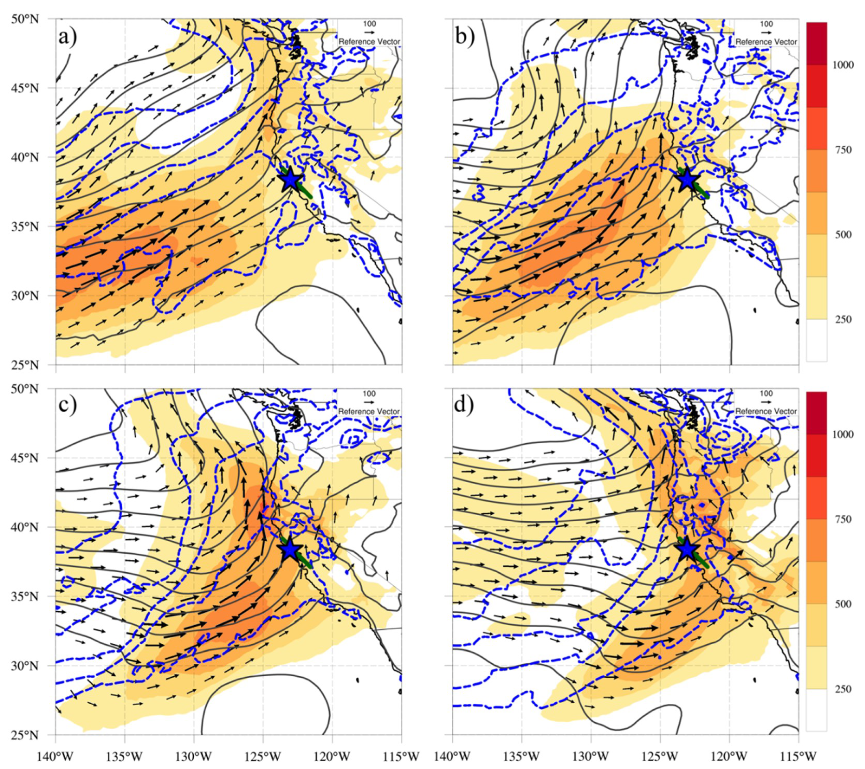
Largescale meteorological feature analysis (
Figure 1) was performed using the North American Regional Reanalysis (NARR) [
23]. Equivalent potential temperature was calculated according to Emanuel, 1994 [
24], and the integrated vapor flux below 1 km MSL was calculated following the formula for IVT in Cordeira et al., 2013 [
20] with the surface pressure and the pressure at 1 km MSL substituted for the lower (upper) limits of integration, respectively.
IVT from NARR and rawinsondes was used as an indicator of AR conditions, with a minimum threshold equal to 250 kg m
−1 s
−1 following Rutz et al., 2014 [
21]. Integrated vapor flux below 1 km is a proxy for orographic precipitation forcing [
25], and its direction can in some cases indicate the presence of terrain-parallel barrier jets [
26,
27]. The equivalent potential temperature was used to diagnose the position and timing of cold fronts [
28].
2.2. Detecting Cloud Layers, Cloud Base, and Below-Cloud Humidity
Cloud layer altitudes, including the base altitude of the lowest cloud, were calculated following Zhang et al., 2010 [
29]. The method uses a profile of saturation with respect to liquid and ice (here provided by rawinsonde) and a set of empirically derived thresholds to identify layers of vertically contiguous cloud while accounting for potential measurement artifacts. Cloud layers were used to inform the calculation of
(see
Section 2.5) and to identify the base altitude of the lowest cloud. Below-cloud relative humidity was then calculated as the mean value reported by rawinsonde below the base of lowest cloud. While crude, this value was used to inform diagnosis of BCE.
2.3. Vapor Sampling and Measurement
A Los Gatos Research (LGR) TWIA-45EP at BBY continuously measured the isotopic composition of surface water vapor using off-axis integrated cavity output spectroscopy. An insulated Teflon tube uniformly heated to 98 °C was used to eliminate condensation during vapor transport to the instrument from the sampling height of 4 m above ground level. Every two hours, an internal reference standard, delivered by a LGR stable water vapor isotope standard source, was measured at varying partial pressures ranging from 9950 to 34,906 ppm to control for humidity-dependent bias in vapor isotope measurements. All water vapor isotope observations fell within this range of partial pressures in the standard measurements. The independent laboratory standard had a δ18O value of −7.23‰ and a δ2H value of −48.70‰ and was independently verified by national and international reference standards: VSMOW2 (δ18O = 0, δ2H = 0), VSLAP2 (δ18O = −55.5, δ2H = −428), USGS45 (δ18O = −2.238, δ2H = −10.3), USGS46 (δ18O = −29.8, δ2H = −235.8), USGS47 (δ18O = −2.224, δ2H = −150.2). This technique produced an error of 0.83‰ (1σ) in δ2H during the measurement of the standard. Values are reported relative to Vienna standard mean ocean water (VSMOW).
2.4. Precipitation Sampling and Measurement
Two Teledyne ISCO model 674 water samplers, connected to 300 mL funnels with Tygon tubing, collected hourly precipitation samples from 00 Coordinated Universal Time (UTC) on 5 March to 00 UTC on 7 March 2016 at BBY. The samplers dispensed precipitation into one of 24 glass bottles for the duration of each hourly collection interval. The samplers were manually activated and programmed to sample sequentially, providing 48 h of continuous precipitation sampling. The LGR TWIA-45EP (Los Gatos Research, San Jose, CA, USA) was used to determine the oxygen and hydrogen isotope compositions of the precipitation samples. Ten injections were made for each measurement and the first five were discarded to eliminate memory effects. Samples were measured in at least triplicate. Measurements were corrected using USGS reference water standards (USGS45, USGS46 and USGS47—see
Section 2.3) and LGR Liquid Water Isotope Analyzer post-analysis software version 3.1.0.9 (Los Gatos Research, San Jose, CA, USA). Temperatures were stable in the analyzer throughout the analysis. This technique produced a standard deviation of <0.2 ‰ in δ
18O and <0.5‰ in δ
2H values. Values are reported relative to Vienna standard mean ocean water (VSMOW).
2.5. Condensation Temperature Diagnosis
The rawinsonde temperature, pressure and water vapor mixing ratio were used to calculate the condensation temperature (T
cond) following the formula
where T and P are the sounding temperature and pressure in Kelvin and Pa, respectively. P
o and P
top refer to the lowest and highest pressure of the sounding, respectively.
The condensation rate
, in kg kg
−1 hr
−1, is calculated by the following assumption: The sounding reported water vapor mixing ratio within any cloud will be adjusted by condensation to the saturated vapor mixing ratio after cooling by moist adiabatic ascent, resulting in the formula
where
w is the ascent in m hr
−1,
qv is the water vapor mixing ratio in kg kg
−1,
qs,l is the saturated mixing ratio with respect to liquid (kg kg
−1) found by Clausius–Clapeyron and
dz is the infinitesimally small change in height in m. We did not have a vertical profile measurement of ascent; therefore, we adopt the assumption that vertical motion follows a constant vertical profile, allowing this variable to cancel in the calculation of T
cond. The condensation rate was set to zero outside cloud layers. Following these methods, T
cond followed changes in the profiles of temperature (through the numerator and Clausius–Clapeyron) and mixing ratio along with the meteorological evolution of the AR.
2.6. Calculating Rainout and Disequilibrium between Precipitation and Surface Vapor
In order to quantify the fraction of rainout (1-
f), we used the framework of open-system Rayleigh distillation [
7]:
where R is the measured isotopic ratio
18O/
16O of precipitation, R
i is the initial measured isotopic ratio of precipitation,
f is the fraction of vapor remaining (to be calculated), and
α is the vapor-liquid equilibrium fractionation factor [
30]. As
α is temperature-dependent, we used the meteorological parameter T
cond to constrain the fractionation factor. Adding in the conversion from precipitation to vapor and formatting in delta notation, the equation above yields:
where δp is the measured δ
18O of precipitation, δv
i is the measured initial δ
18O of vapor and
lnα is the natural logarithm of the fractionation factor
α. As this approach assumes a perfectly open system without interaction between falling hydrometeors and surrounding atmosphere, we only applied this calculation to times during the AR event lacking a large influence of post-condensation processes (see
Section 3). Also critical to this approach is the assumption that the vapor from which precipitation is forming is related to the vapor measured at the surface. Yoshimura et al., 2010 modeled a negative vertical isotope gradient in the atmosphere, with δv values near zero at the surface and decreasing aloft [
18]. Thus, the estimates of rainout (1-
f) presented here are likely upper bound estimates and, as such, relative changes in the degree of rainout should be interpreted with greater importance than absolute values.
To assess the degree of disequilibrium between precipitation and surface vapor, we first translated the isotopic composition of vapor (δv) into equilibrium precipitation from vapor (δp
eqv) using the vapor–liquid equilibrium fractionation factor of Majoube, 1971 [
30] and the temperature at condensation height (T
cond). Next, we computed the difference between the oxygen isotope composition of actual precipitation (δp) with this vapor-reconstructed precipitation (δp
eqv) in order to quantify the degree of disequilibrium (δp−δp
eqv). As discussed above, some degree of disequilibrium is expected due to the vertical gradient in δv. As we did not measure water vapor isotopes aloft, we cannot distinguish between changes in the vertical isotope gradient and other causes of disequilibrium such as Rayleigh distillation and post-condensation processes.
While we believe Tcond is the superior constraint on the temperature of fractionation as it is our best estimate of the temperature conditions where the phase change is occurring, it is possible to conduct the same calculations using surface temperatures (Tsurf). As a point of comparison, here we discuss the use of Tcond vs. Tsurf for the calculation of vapor-reconstructed precipitation (δpeqv) and the degree of disequilibrium (δp−δpeqv). Throughout the event, Tcond averaged 276 K while Tsurf was 10 degrees warmer at 286 K. Using Tsurf instead of Tcond, δpeqv was 12.8‰ lower on average in δ2H values and 0.9‰ lower in δ18O values. These decreases in δpeqv derived from Tsurf produce differences in the calculated degree of disequilibrium. Thus, using Tsurf instead of Tcond would reduce the degree of disequilibrium (δp−δpeqv). As these differences are systematic, the use of Tsurf or Tcond would not drive changes to our interpretation.
In fact, we find it more likely that T
cond overestimates temperature and therefore underestimates fractionation. There may be an isotopic imprint of colder condensation temperatures (above the cloud base). Making this effect even more significant would be the impact of fractionation between vapor and ice, which is greater than the fractionation between vapor and liquid [
31]. Thus, our calculated degree of disequilibrium may be an underestimate of one derived from more well-constrained meteorological conditions. Nonetheless, while imperfect, we choose to use T
cond as our meteorological constraint as we believe it reflects the best estimate available of the temperature conditions at the point of condensation.
3. Stable Isotope and Meteorological Chronology
AR conditions were first recorded at BBY on 4 March 2016 (
Figure 1a). However, a significant relaxation of IVT occurred shortly thereafter and IVT did not increase again until near 15 UTC on 5 March 2016 (see Martin et al., 2018 [
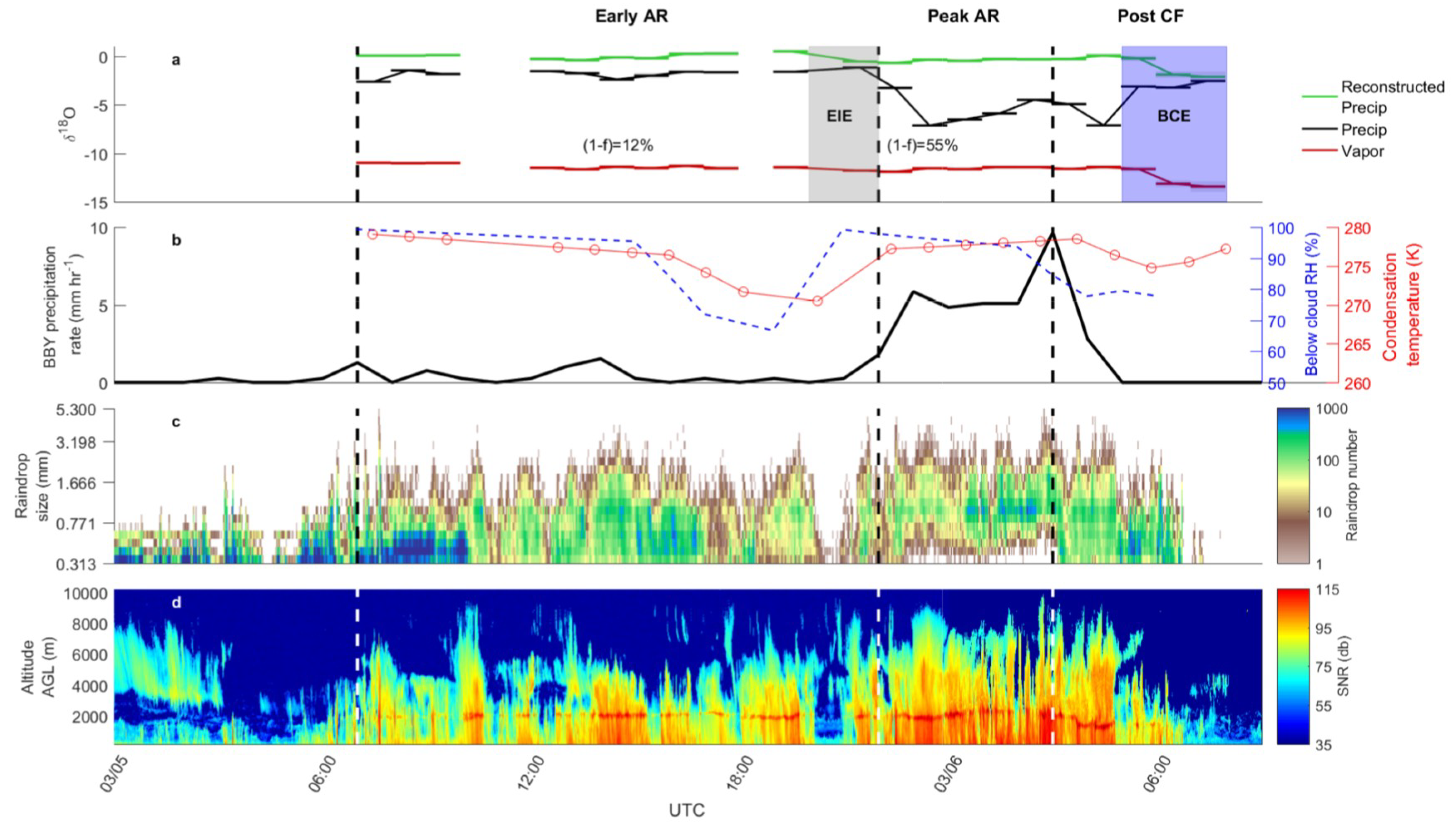
27] for a more detailed description of the evolution of AR conditions). Precipitation began to fall at BBY at 7 UTC on 5 March, but precipitation rates remained low (<3 mm hr
−1) until 22 UTC on 5 March (
Figure 2b). During this early AR period, cloud structure was inconsistent with an intermittent brightband radar signature (
Figure 2c,d). δp and δp
eqv remained stable for most of this period, fluctuating <1.5 ‰ in δ
18O (
Figure 2a). The disequilibrium between the two reflects the typical vertical isotope gradient in the atmosphere. During this period, 1-
f averaged 11.9 ± 2.6%.
During the period 15 UTC to 21 UTC on 5 March (
Figure 1b,c), IVT progressively increased to nearly 750 kg m
−1 s
−1, and vapor flux below 1 km MSL increased and turned parallel to the coastal mountain terrain. A coastal barrier jet was present during this time period, with maximum strength at 21 UTC on 5 March [
27]. At the end of this period, between 20–22 UTC on 5 March, the cloud structure broke down and rain droplet size decreased to below disdrometer measurable sensitivity. During this phase, δp and δp
eqv closed to within 0.7‰ due to increased EIE of small falling droplets with saturated below-cloud vapor (
Figure 2b).
The precipitation rate increased rapidly after 22 UTC on 5 March, and remained high through the passage of the cold front around 3 UTC on 6 March. A rawinsonde indicated peak IVT (956 kg m
−1 s
−1) was reached over BBY near 01 UTC on 6 March. During this peak AR period, clouds exhibited a consistent brightband and the low-level jet, responsible for the majority of terrain-normal vapor flux, reached its maximum. Between 22 UTC on 5 March and 1 UTC on 6 March, δp rapidly dropped by 6‰ while δp
eqv remained constant, suggesting that this decrease was caused by an increase in rainout (1-
f). At this minimum δp, 1-
f reached 54.8%. δp increased by 2.6‰ over the first few hours of 6 March, as the initial rain rate and droplet sizes stabilized, until δp reached a local maximum just before the leading edge of the cold front reached BBY at 3 UTC on 6 March (
Figure 1d).
The cold front passage was accompanied by a spike in precipitation rate to the highest recorded during the event. As rainfall spiked, δp decreased back to the previous minimum value recorded during the peak AR period. However, the increased storm intensity of this post-cold front period was short-lived. IVT decreased rapidly offshore and, subsequently, at BBY as the weather system moved inland. Precipitation rates and droplet size decreased and the brightband disappeared by 5 UTC on 6 March. This was accompanied by a rapid closing of δp and δp
eqv during which δp increased by >4‰ between subsequent hour samples, the highest rate of change observed during the event. As below-cloud RH was ~80% (
Figure 2a), we conclude that BCE drove this rapid shift, as droplets evaporated into an unsaturated below-cloud air mass. Rawinsondes indicated that AR conditions over BBY ended after 06 UTC on 6 March.
In the above section, we focused exclusively on δ
18O values as oxygen and hydrogen isotope values vary sympathetically. Due to the ratio of the oxygen and hydrogen fractionation factors, precipitation typically falls along the meteoric water line: δ
2H = 8δ
18O +
d, where
d is the deuterium excess [
32]. This explains the close relationship between hydrogen and oxygen isotopes in precipitation and vapor, though hydrogen isotope values vary by ~8 times that of oxygen (
Figure 3a,b). As in δ
18O
p, the δ
2H
p time series displays equally prominent “V” shaped variations while these trends are markedly absent in vapor. This confirms that the processes driving the “V” shapes are not related to the large-scale advection of moisture, such as changing moisture sources within the precipitation event. Instead, these processes must be local and driven by meteorological dynamics and microphysical processes.
Figure 3c depicts the deuterium excess of precipitation and vapor, defined as
d = δ
2H – 8δ
18O [
7]. This quantity arises due to the kinetic fractionation during evaporation and relates to the relative humidity, with high
d values associated with low relative humidity (RH) and low
d values associated with high RH. Deuterium excess of precipitation reveals some interesting trends. First, from 15–20 UTC on 5 March,
d of precipitation exhibited a trough, driven by low RH and strong BCE. This abruptly terminated as RH returned to 100% between 20–22 UTC with a rapid increase in
d, consistent with BCE shutting off and EIE dominating. This interpretation is supported by the convergence of precipitation and reconstructed precipitation (
Figure 2).
d decreases then increases and peaks at the cold frontal passage at 3 UTC on 6 March. Deuterium excess during this portion of the storm is particularly variable. This may be an artifact of our binned samples or indicative of the variable role that post-condensation processes play during the event. Following cold frontal passage, both RH and
d drop, consistent with the return of BCE. Deuterium excess of vapor is less variable than precipitation and exhibits a modest increase from ~3 to ~10 throughout the event. This trend, while weak, likely reflects changing moisture sources from a the warm, moist, low-latitude source of the storms warm sector (the warm, moist air mass including the AR core in advance of the cold front) to the cooler, drier, midlatitude source of the cold sector (behind the cold front). A similar pattern has been observed in the North Atlantic, with high
d values associated with more northern storm tracks and evaporation at a low-RH moisture source [
33].
4. Discussion
Stable isotopes in precipitation can provide a wealth of insight into the processes driving (and modifying) precipitation. In the 5–7 March 2016 AR event in northern California, we observed a decrease and re-enrichment of ~6‰ in δ
18O of precipitation organized into a prominent “V” shape, not unlike those observed in other ARs [
6,
34] and precipitation events more broadly [
1,
11,
12,
35,
36,
37,
38,
39,
40]. We observe a “V” with an asymmetric shape, with higher δp values in the period before the “V” than after, a signature of cold frontal passage [
19]. Unlike the initial interpretation of the 2005 landfalling AR, in which Coplen et al. argued that changes in cloud height and temperature drove large isotopic changes, here, we find no evidence that temperature played a major role [
6]. The temperature lapse rate was nearly invariant, staying very close to the moist adiabatic lapse rate below 6 km. Condensation temperature (
Figure 2b) ranged from 269–279 K throughout the event, corresponding to a maximum change of 1.1‰ in δ
18O vapor-liquid fractionation. This variability is greatly overshadowed by the large changes observed in the stable isotope time series of this AR event (
Figure 2a). Thus, the stable isotope and meteorological chronologies of the March 2016 AR tell a complex, yet coherent story. Here, we discuss the evidence for the changing roles of meteorological structure and post-condensation processes in driving and modifying the rainout of atmospheric moisture.
The initially high values of δp are set by a relatively small degree of rainout (1-f = 12%) during the early period of the AR, before the coastal barrier jet arrived at BBY. This phase terminates as the coastal barrier jet strengthens, dynamically lofting moisture from the AR low-level jet. Isotopically, this termination phase is characterized by convergence between δp and δpeqv, indicating equilibration between precipitation and vapor. This equilibration is likely the result of equilibrium isotope exchange, as the cloud structure breaks down and droplet sizes and precipitation decrease while the airmass remains saturated, thereby suppressing evaporation.
Following the termination of the early AR phase, the low-level jet strengthens while the barrier jet remains strong driving extreme rainout (1-f = 55%) during peak AR conditions. This manifests as an abrupt drop of 6‰ in δp over just two hours and an isotopic regime driven by open-system Rayleigh distillation. This suggests that the dynamic lofting of the moist AR core over the coastal barrier jet can create highly efficient rainout, likely via the seeder-feeder mechanism. After the cessation of the barrier jet near 00 UTC on 6 March, orographic lifting of the low-level jet by the nearby coastal mountain ranges created similarly efficient removal of atmospheric moisture.
Peak AR conditions abate two hours after cold frontal passage, leading to the termination of seeder-feeder clouds and decreased drop size, precipitation rate and relative humidity. Isotopically, this period is characterized by a rebound of 4.5‰ likely driven by below-cloud evaporation given the large oxygen isotope increase and low relative humidity. As in the case of equilibrium isotope exchange at the termination of the early AR phase, below-cloud evaporation overprints the initial isotopic composition of precipitation most effectively during periods characterized by low precipitation rate and small drop sizes [
13].
How do the findings of the 5–7 March 2016 AR event relate to the broader discussion on isotope signatures of precipitation events? First, Rayleigh distillation is still the governing theory of isotopes in precipitation, particularly when examining the hydrologic cycle at large spatial or temporal scales. Ignoring the role that post-condensation processes play in AR events [
6,
34], however, is a mistake, as both paired water–water vapor isotope records (this study) and isotope-enabled GCMs [
18,
19] have shown. Post-condensation processes play a significant role in AR events, though they are easily dwarfed by Rayleigh distillation during the periods of most consequential rainfall. We do not, however, see evidence in the March 2016 AR event that BCE played a role in the initial enrichment and subsequent drop in precipitation as argued by Yoshimura et al. in the March 2005 AR [
18]. Instead, we attribute the stable isotope signature near the end of the early AR period to be the result of equilibrium isotope exchange immediately prior to the lofting of the AR core over the coastal barrier jet. Only the re-enrichment phase was driven by BCE. Therefore, we argue that the rebound portion of the prominent “V” shapes observed in cold frontal systems worldwide are likely driven by post-condensation processes.


