Study on the Construction of Initial Condition Perturbations for the Regional Ensemble Prediction System of North China

Institute of Urban Meteorology, China Meteorological Administration, Beijing 100089, China
*
Author to whom correspondence should be addressed.
Atmosphere 2019, 10(2), 87; https://doi.org/10.3390/atmos10020087
Submission received: 7 November 2018
/
Revised: 2 February 2019
/
Accepted: 5 February 2019
/
Published: 19 February 2019
(This article belongs to the Special Issue Numerical Weather Prediction, Data Assimilation and Ensemble Forecasting—EGU 2018 Session)
Abstract
:The regional ensemble prediction system (REPS) of North China is currently under development at the Institute of Urban Meteorology, China Meteorological Administration, with initial condition perturbations provided by global ensemble dynamical downscaling. To improve the performance of the REPS, a comparison of two initial condition perturbation methods is conducted in this paper: (i) Breeding, which was specifically designed for the REPS, and (ii) Dynamical downscaling. Consecutive tests were implemented to evaluate the performances of both methods in the operational REPS environment. The perturbation characteristics were analyzed, and ensemble forecast verifications were conducted. Furthermore, a heavy precipitation case was investigated. The main conclusions are as follows: the Breeding perturbations were more powerful at small scales, while the downscaling perturbations were more powerful at large scales; the difference between the two perturbation types gradually decreased with the forecast lead time. The downscaling perturbation growth was more remarkable than that of the Breeding perturbations at short forecast lead times, while the perturbation magnitudes of both schemes were similar for long-range forecasts. However, the Breeding perturbations contained more abundant small-scale components than downscaling for the short-range forecasts. The ensemble forecast verification indicated a slightly better downscaling ensemble performance than that of the Breeding ensemble. A precipitation case study indicated that the Breeding ensemble performance was better than that of downscaling, particularly in terms of location and strength of the precipitation forecast.
1. Introduction
Numerical weather prediction (NWP) has great uncertainty due to the initial condition (IC) error, model error and chaotic nature of the atmosphere; thus, the ensemble forecast method, which is a practical way to provide probabilistic forecasts, has been proposed [1]. Since the ensemble prediction system (EPS) was originally implemented in the early 1990s at the National Centers for Environmental Prediction (NCEP) [2] and the European Centre for Medium-Range Weather Forecasts (ECMWF) [3], several meteorological centers have subsequently constructed their own operational EPSs [4,5,6].
The forecasting of mesoscale severe weather, such as heavy precipitation, local convective systems and thunderstorms, is an important aspect of regional NWP. Because the mechanisms of such mesoscale and small-scale phenomena are very complicated, developing a regional ensemble prediction system (REPS) seems to be an effective means of solving this problem.
The means by which to generate IC perturbations for a REPS is a critical issue. One option is global EPS dynamical downscaling, which involves the interpolation of forecast fields from a set of representative global EPS members to the regional domain with a higher resolution. This method has been successfully applied in some of the current operational REPSs [7,8,9,10,11,12,13,14]. Although dynamical downscaling is attractive for its simplicity and suitable performance, regional small-scale uncertainties cannot be explicitly represented with dynamical downscaling [15]. Other studies have attempted to generate IC perturbations for the REPS using regional versions of the traditional IC perturbation methods originally applied to the global ensemble, including Breeding Growing Mode (BGM) [16], Singular Vectors (SVs) [17], Ensemble Transform Kalman Filter (ETKF) [18], and so on. Additionally, these methods are practical for a REPS [19,20,21,22].
However, thus far, it remains unclear whether these regional versions of IC perturbation methods, as primarily designed for medium-range forecasting, are superior to downscaling when applied to a REPS. Bowler and Mylne [23] tested the ETKF method and downscaling in a regional version of the Meteorological Office Global and Regional Ensemble Prediction System (MOGREPS) and revealed that the perturbations generated by a regional ETKF were more detailed at small scales and had lower accuracy at large scales with less than an 18 h forecast lead time. These perturbations are smaller overall than the perturbations derived from downscaling, and the performances of the two ensembles are very similar, with a slightly better performance observed from downscaling. The results comparison presented by Saito et al. [24] is mixed, as the downscaling method tends to perturb the synoptic-scale flow and has the best spread and RMSE results, while the regional BGM and SV tend to perturb mesoscale circulation, and therefore, affect the local intense rains to a greater extent. Zhang et al. [25] tested the ETKF method and downscaling in the CMA (China Meteorological Administration) operational REPS environment and concluded that downscaling is better than the ETKF at spread growth but lacks small-scale information. There seems to be no clear conclusion as to which of these regional IC perturbation methods is optimal for a REPS, and different operational centers determine how to use the perturbation method according to the needs of each center.
Since May 2014, the Institute of Urban Meteorology of the CMA has been developing a specific REPS for North China, with the IC perturbations generated by dynamical downscaling from an operational global ensemble forecast system (GEFS) [26]. Because this REPS is aimed at local weather phenomenon prediction, a more effective perturbation method other than dynamical downscaling should be tested. Because the system has two initialization times each day, it is possible for the REPS to generate IC perturbations from the Breeding cycle. A detailed comparison of the IC perturbation methods of Breeding and downscaling for the REPS of North China are provided in this study. Our aim is to improve understanding of the advantages and disadvantages of both IC perturbation methods for the REPS, and this investigation is also expected to provide information for future REPS improvements.
The outline of this article is as follows. The system, IC perturbation principle, experimental set-up, and verification method are described in Section 2. The perturbation quality evaluation and ensemble tool verification results and discussions are presented in Section 3. Additionally, a case of heavy precipitation in the North China region is investigated. Finally, a summary of the obtained results and conclusions are provided in Section 4.
2. System and Method
2.1. Introduction of the Regional Ensemble Prediction System of North China
REPS research has been conducted in several operational centers in China, such as the REPS in the Numerical Weather Prediction Center of the CMA, the REPS in the Shanghai Typhoon Institute of the CMA and the REPS in the Institute of Tropical and Marine Meteorology of the CMA. The REPS of North China was developed to meet the probability forecasting requirements of local severe weather for North China and is now running quasi-operationally in the Institute of Urban Meteorology of the CMA.
This REPS is constructed based on a regional model of Weather Research and Forecasting (WRF), Version 3.8 [27]. To save computational costs, only one domain is used without nesting in the model, and this domain covers most of northeast China with a spatial resolution of 6 km × 6 km (274 × 209 grid cells) (Figure 1). The number of model sigma coordinated levels is set to 51 vertically with the top as high as 50 hPa. Considering that the uncertainty related to the physical parameterizations is a complex issue [28], no model perturbations are introduced in this paper, and the main model physics configuration of all members are identical to that of the operational deterministic forecast, i.e., Thompson microphysics, Kain-Fritsch Cumulus parameterization, Mellor-Yamada-Janjic (MYJ) planetary boundary layer (PBL) scheme and RRTMG longwave and shortwave radiation schemes.
Because the REPS of North China has been coupled with the GEFS of the NCEP, the IC perturbations of this REPS are generated by dynamical downscaling of the GEFS. The lateral boundary conditions (LBCs) are also represented by those of the GEFS without feedback. The REPS consists of 21 members including a control run and 20 perturbed members. The system is started at 0000 UTC and 1200 UTC every day, and the longest forecast range is 36 h for each start time.
2.2. Introduction of the IC Perturbation Schemes
It is critical to choose the correct IC perturbation method for a REPS. As mentioned in the introduction, one common means of choosing the correct method is to downscale the global ensemble IC perturbations to obtain regional ensemble IC perturbations, while other methods generate IC perturbations using traditional perturbation methods, such as Breeding, to generate IC perturbations for a REPS. There is no definite conclusion as to which of the two methods is superior. As mentioned above, the North China REPS developed by the Institute of Urban Meteorology of the CMA generates IC perturbations by dynamical downscaling. The main drawback of this method is that the approach cannot generate sufficient small-scale perturbation components to represent the uncertainty of small-scale weather. Therefore, we attempt to adopt the Breeding method in this paper based on the regional model’s own cycle. In this section, a brief introduction of the methods of dynamical downscaling and Breeding is presented.
2.2.1. Downscaling
The traditional downscaling mechanism is a process aimed at determining the mathematical relation between the global and local fields [29]. There are a variety of downscaling techniques in the literature, but two major approaches are currently identified, i.e., dynamical downscaling and empirical (statistical) downscaling. The dynamical downscaling approach is a method of extracting local-scale information by regional models with coarse global data used as the boundary conditions [30]. For a regional ensemble forecast, the dynamical downscaling process interpolates an ensemble of global ICs to the regional model domain and resolution to obtain regional ensemble IC perturbations [13]. Generally, this approach is attractive due to its simplicity and practicality, and the downscaling method in this paper mainly refers to dynamical downscaling.
2.2.2. Breeding
The Breeding method is an IC perturbation method commonly used in ensemble prediction. The theoretical basis is that in the daily operational cycle of the data assimilation process and the error of the analysis field have random, nongrowing components, and there are also well-organized, rapidly growing error components that have a large impact on the forecast. Toth and Kalney [16] designed a method for IC perturbation generation that simulates the error growth process in the analysis cycle and provides a fast-growing perturbation structure through cycling. This method has received extensive attention and application because of its clear scientific and theoretical basis, good results, and low computational cost.
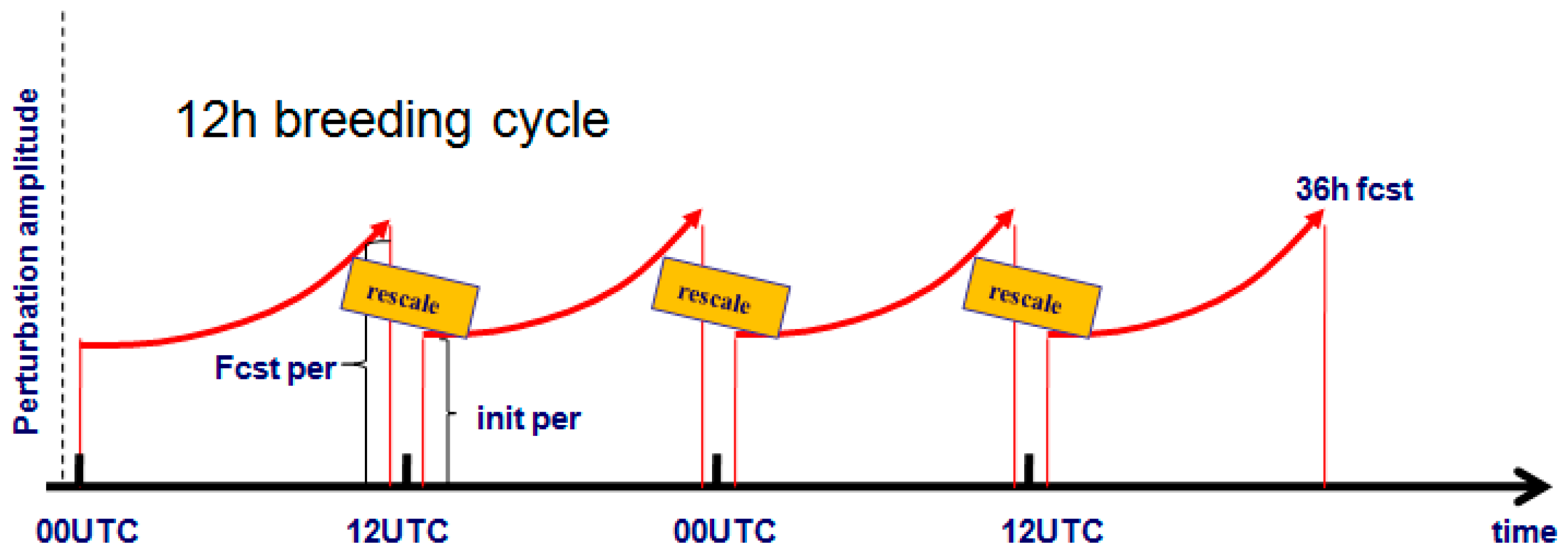
A Breeding method is applied to compute IC perturbations of the North China REPS, with a 12 h Breeding cycling interval. For each initial time, the forecast perturbations of the previous Breeding cycle are rescaled to mathematically obtain the IC perturbations of the present cycle, which is as follows:
where represents the IC perturbations at grid point i,j at a particular level, represents the corresponding forecast perturbations, and is a rescaling factor that rescales the perturbation amplitude to ensure that the IC perturbation amplitude is suitable to represent the initial uncertainties. Because we can obtain the corresponding downscaling perturbations simultaneously, here, we assume that the amplitudes of the downscaling perturbations can represent the initial uncertainties; therefore, the rescaling factor calculation is determined by referencing the amplitudes of the downscaling perturbations, which is as follows:
where represents the downscaling IC perturbations at grid point i,j within an m × n horizontal dimension. As this calculation can obtain an R value for each model level, here, we define the average R value at all model levels as the final rescaling factor to be used in Equation (1). It is not difficult to understand that the amplitudes of the Breeding IC perturbations and downscaling IC perturbations are comparable after the rescaling process of Equation (1).
For each Breeding cycle, to center the IC perturbations of twenty perturbed members around the control, 10 members (half of the 20 perturbed members) of the previous cycle are randomly selected to provide forecast perturbations, and 10 IC perturbation groups are obtained after rescaling. Then, these 10 rescaled perturbations are added to (or subtracted from) the IC perturbations of the control; thus, the IC perturbations of the first (or last) 10 of the 20 ensemble members are obtained. The IC perturbations for the 20 perturbed members are positive-negative paired. Five variables (zonal wind u, radial wind v, potential temperature θ, pressure π and specific humidity q) are perturbed in the ICs.
The Breeding method cycling process is as follows: the system starts at 00:00 UTC and 12:00 UTC every day. For each initial time, the system provides a 36 h ensemble forecasting product, and the 12 h forecast perturbations are used to calculate the IC perturbations of the next cycle. The latter is realized by the rescaling factor mentioned above. The flow chart of the Breeding cycle is shown in Figure 2.
2.3. Experimental Set-Up
In the present study, the Breeding and downscaling methods are both compared in the same REPS configuration. Two sets of regional ensembles are constructed with IC perturbations generated by Breeding and downscaling, and no model perturbations are introduced in this study. The system settings of the two tests are identical. The background states and LBCs for the REPS are provided by GEFS global ensemble forecast data with a horizontal resolution of 1 degree Celsius.
The two different ensembles compared in this work will be denoted as Breeding and Down. A one-month period from 1 May 2017 to 31 May 2017 is chosen for this comparison. The 36 h forecast lead times are evaluated. The GFS global analysis states corresponding to each forecast lead time are used to verify the upper air variables, while the precipitation is verified against observational accumulative precipitation data from 2507 meteorological stations in China.
2.4. Verification Methods
Multiple methods are applied in this study to evaluate the performance of ensemble forecasts, including probability verification scores and deterministic verification scores.
Before the analysis of the ensemble perturbation characteristics, the ensemble perturbation definition is provided. For a certain grid within an m × n domain, and with a grid ID of i and j, the perturbation for this grid is as follows:
where N is the ensemble size, is the member forecast, and refers to the control. The scale characteristic analysis and perturbation evolution study are based on this definition.
A useful measure of the performance of a REPS is how well the ensemble spread matches the root mean square error (RMSE) of the ensemble mean [31]. The ensemble spread and RMSE of the ensemble mean are also applied in this study, and are calculated as follows:
where m and n are the total number of grids, and refers to the ensemble mean; the RMSE of the ensemble mean is as follows:
where refers to the analysis.
Another measure of statistical reliability is the Talagrand diagram [32]. This measure is a statistic of the frequency at which the observation lies inside or outside the whole ensemble. A more reliable EPS should have a flatter pattern. A U-shape indicates a lack of spread, while J or L-shapes indicate the presence of bias in the system.
Additionally, we use the threat score (TS) to evaluate the precipitation forecasting ability of the two ensembles. As defined by Gilbert [33], the TS is given by the following:
where a is the hit rate, b is the false alarm rate, and c is the miss rate.
3. Results and Discussion
We now evaluate the perturbation quality and ensemble forecast accuracy for the two ensembles. First, it is desirable for a REPS to provide uncertainty information at all scales, not only at synoptic scales, but also at convective scales; therefore, we begin with an examination of the scale characteristics of the Breeding and Down perturbations. In addition, since the ensemble spread growth is closely correlated with the perturbation growth, we investigate how the perturbation patterns evolve. Thereafter, we assess the ensemble forecast performance through a series of probability verification methods. A precipitation case study is also presented to evaluate the practicability of the two methods.
3.1. Power Spectra Analysis
A suitable ensemble forecast can provide sufficient uncertainty information, not only for small-scale information, but also for large-scale information. The scale characteristics of both the Breeding and Down perturbations are investigated by calculating the power spectra. Here, we use a 2-dimensional discrete cosine transform (2D-DCT), which is suitable for the spectral analysis of data in a limited area [34]. The power spectra are calculated for the perturbations defined in Formula 3.
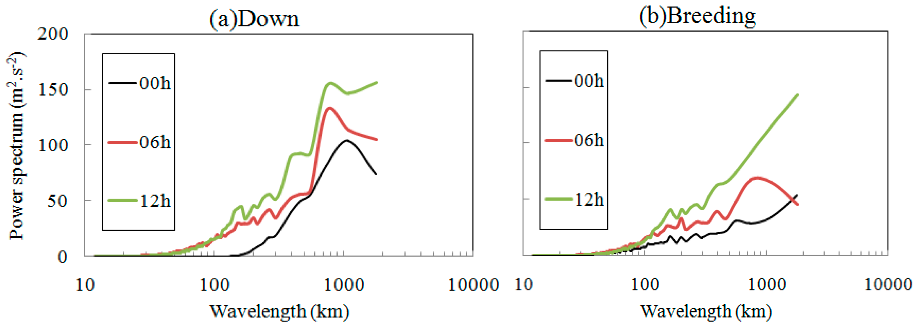
Figure 3 shows the power spectra of the 500 hPa zonal wind perturbations as a function of the wavelength for both the Breeding ensemble and Down ensemble. The power spectra of the initial perturbations (00 h), 06 h and 12 h forecast perturbations are presented. The results from the initial (00 h) forecasts (black lines) indicate that the performances of the Breeding perturbations are better than those of the Down perturbations at wavelengths of less than 110 km, which is the grid space of the GEFS downscaling state. Because these scales cannot be resolved by the global model, the Down perturbations derived from the global ensemble exhibit no power at these length scales. For scales beyond 110 km, greater power can be obtained in the Down ensemble, as the maximum power spectrum value reaches 100 m2·s−2 (corresponding to a wavelength of 1000 km), while the maximum value for the Breeding ensemble only reaches 50 m2·s−2 (corresponding to a wavelength of 2000 km). The scale characteristics of the Down perturbations with 6 and 12 h forecast lead times (Figure 3a) indicate that the downscaling perturbations have increased the power spectra compared to those of 00 h at all length scales, including small-scale perturbations. The 6 h and 12 h Breeding perturbations exhibit amplified power spectra compared to those of 00 h at all scales, particularly at large scales; and the most powerful scale for the 12 h forecast is 2000 km, with a power spectrum value of 100 m2·s−2.
The results presented above indicate that the perturbations generated by the two methods have substantial differences in scale. For the Breeding method, because the IC perturbations are generated through cycling mechanisms within the regional model, the method can produce sufficient small-scale components at the initial time of each cycle; therefore, the Breeding perturbations are better at representing the convective, high impact weather uncertainty for short range forecasting. However, the downscaling perturbations lack small-scale components at the initial time, but the advantage of such perturbations is evident at a larger scale.
3.2. Perturbation Growth Characteristics
The growing forecast error is a key feature that affects the forecast quality, and suitable ensemble perturbations should properly represent these growing forecast errors. To investigate the perturbation characteristics intuitively, an attempt has been made to analyze the distribution and evolution characteristics of the perturbations.
First, it is desirable to compare both ensembles in terms of the perturbation magnitude. We average the perturbations at all grid points at each level to obtain the vertical profiles of perturbations. Figure 4 illustrates such perturbation profiles with 0-36 h forecast lead times for the zonal wind. Figure 4a shows that the Down ensemble perturbations can maintain a steady growth with the forecast lead time, and the most remarkable growth level is the 27th model level (approximately 250 hPa). For example, the perturbation magnitude at the 27th level is 1.7 m·s−1 at the initial time, while at the 12 h lead time, the corresponding value is 3 m·s−1; the perturbation growth slows as the forecast lead time increases. For the Breeding ensemble, the perturbation growth characteristics are similar. The largest perturbation can also be found at the 27th level, and the initial perturbation value is 1.7 m·s−1, which is similar to that of the Down ensemble, while the corresponding value is 2.7 m·s−1 for the 12 h forecast lead time. Notably, the perturbation magnitude of the Breeding ensemble is always smaller than that of the Down ensemble at different forecast lead times, except for the upper level at the initial time; the difference between the two systems gradually decreases with the extension of the forecast time (see Figure 4c).
Figure 5 shows the horizontal distributions of the zonal wind averaged over all members at 500 hPa for both the Down and Breeding ensembles. For the Down ensemble, analysis of the perturbation (Figure 5a) distribution indicates clear large-scale characteristics, given that the maximum value is located in the Central Inner Mongolia Province. For the Breeding ensemble, the initial perturbations (Figure 5d) are generally lower than that of the Down ensemble. Additionally, the Breeding IC perturbations exhibit more abundant small-scale characteristics compared to the Down ensemble perturbations, and this difference also reflects the analytical results shown in Section 3.1.
For the 12 h forecast lead time (Figure 3b,e), the perturbations for both ensembles exhibit remarkable growth, and the large perturbation areas for both schemes correspond well (see East Inner Mongolia and Shanxi). With increasing forecast lead time, the perturbation patterns for both ensembles become similar. The results indicate that the difference between the two systems in the perturbation distribution pattern for short-range forecasts is more significant than that of the long-range forecasts.
3.3. Ensemble Verification Results
3.3.1. Root Mean Square Error and Ensemble Spread
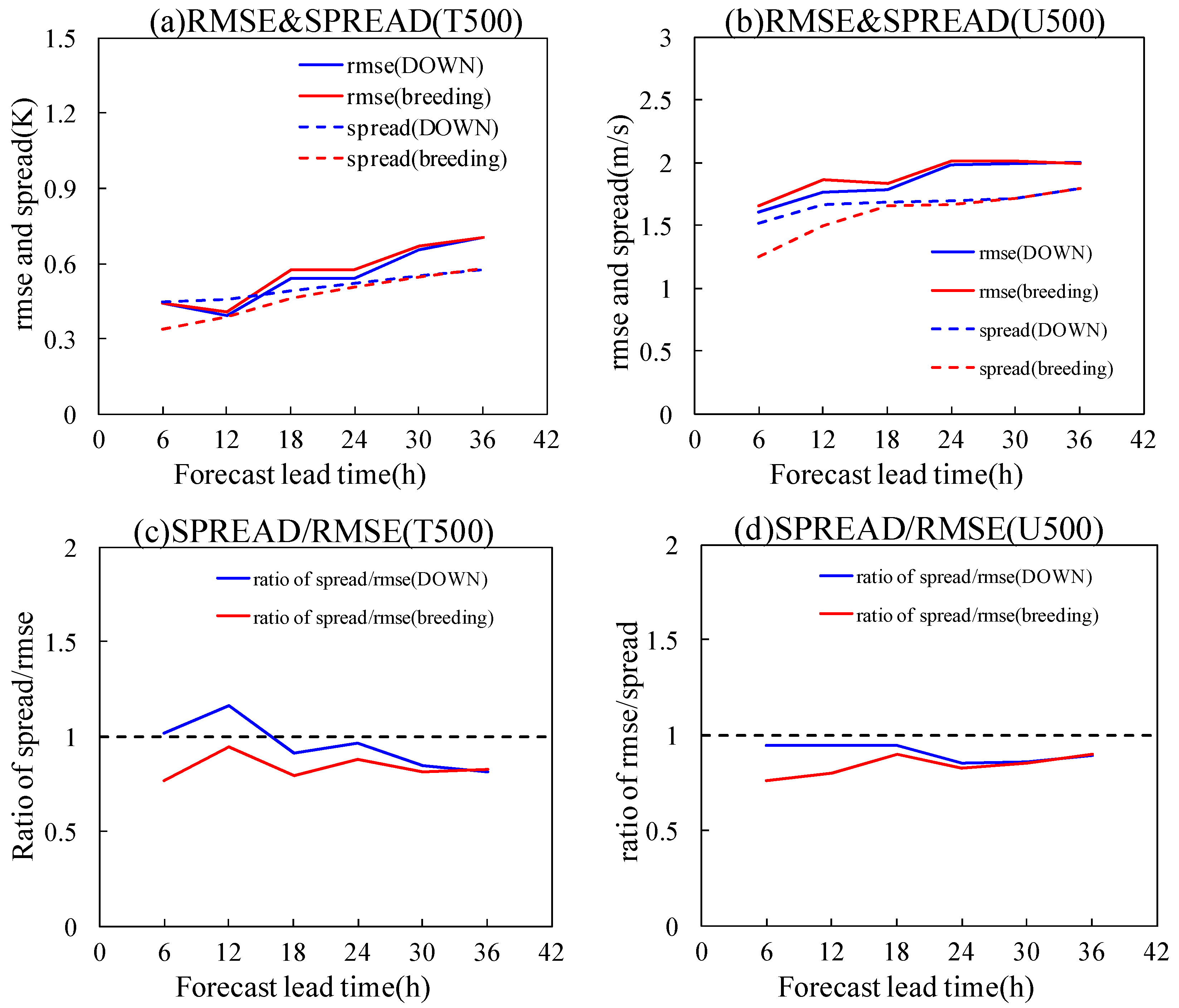
A useful measure of the performance of a REPS is how well the ensemble spread matches the root mean square error (RMSE) of the ensemble mean. Figure 6 shows the one-month averaged RMSE of the ensemble mean and spread, as well as the ratio of the spread and RMSE. For both methods, two upper air variables, namely, the 500 hPa zonal wind (U500) and 500 hPa temperature (T500), are presented for comparison. Both methods have a sufficient spread at short forecast lead times, and the spread growth is slower than the RMSE growth for both ensembles. Taking Figure 4a as an example, for the Down ensemble, the 6 h RMSE of T500 is 0.45 K, while the spread is the same; for the Breeding ensemble, the 6 h RMSE of T500 is 0.45 K, while the spread is 0.33 K, exhibiting characteristics of underspreading. The RMSE and spread are much closer for the Down ensemble within 30 h forecast lead times (see Figure 4c,d), but the two ensembles become very similar beyond a 30 h forecast lead time. Similar results can also be observed for other variables at different pressure levels (not shown). These results suggest that the Down ensemble can truly enhance the reliability of ensemble forecasts at short forecast lead times.
3.3.2. Box Plot of a Single Station
The RMSE and spread verification show that the Down scheme performs well for upper air variables. For near-surface variable forecasting, the performance of the two methods requires further analysis. Figure 7 shows the box plot of the 2 m temperature forecast for a single Beijing station with Down and Breeding schemes. The two sets of forecasts are initiated at 12 UTC on 12 May 2017. Figure 7 shows that since both ensembles have no near-surface initial perturbations, there is almost no divergence at 00 h. With the extension of forecast lead time, the forecast of each member gradually disperses. The probability range of the Down scheme is wide (Figure 7a). The observation falls among the forecasts of all members but remains a certain distance from the ensemble mean and median. For the 18–30 h forecast lead time in particular, the ensemble probability forecasts are generally higher than the observations. For example, for the 24 h forecast, the forecast ranges of the members are 17–20.5 degrees Celsius, the ensemble mean and median are 18 degrees Celsius, and the observation is 17.2 degrees Celsius. For the Breeding scheme, the forecast dispersion is smaller than the that of the Down scheme, but the forecast members are evenly distributed around the observation, and the ensemble mean and median are closer to the observation. For example, for the 24 h forecast, the ensemble member forecast range is 16–19 degrees Celsius with a mean value of 17.5 degrees Celsius, and the observation is 17.2 degrees Celsius. These results indicate that a large ensemble spread does not indicate an improved forecast quality. For near-surface element forecasting, the forecast distribution of each member of the Breeding method is more reasonable.
3.3.3. Talagrand Diagram
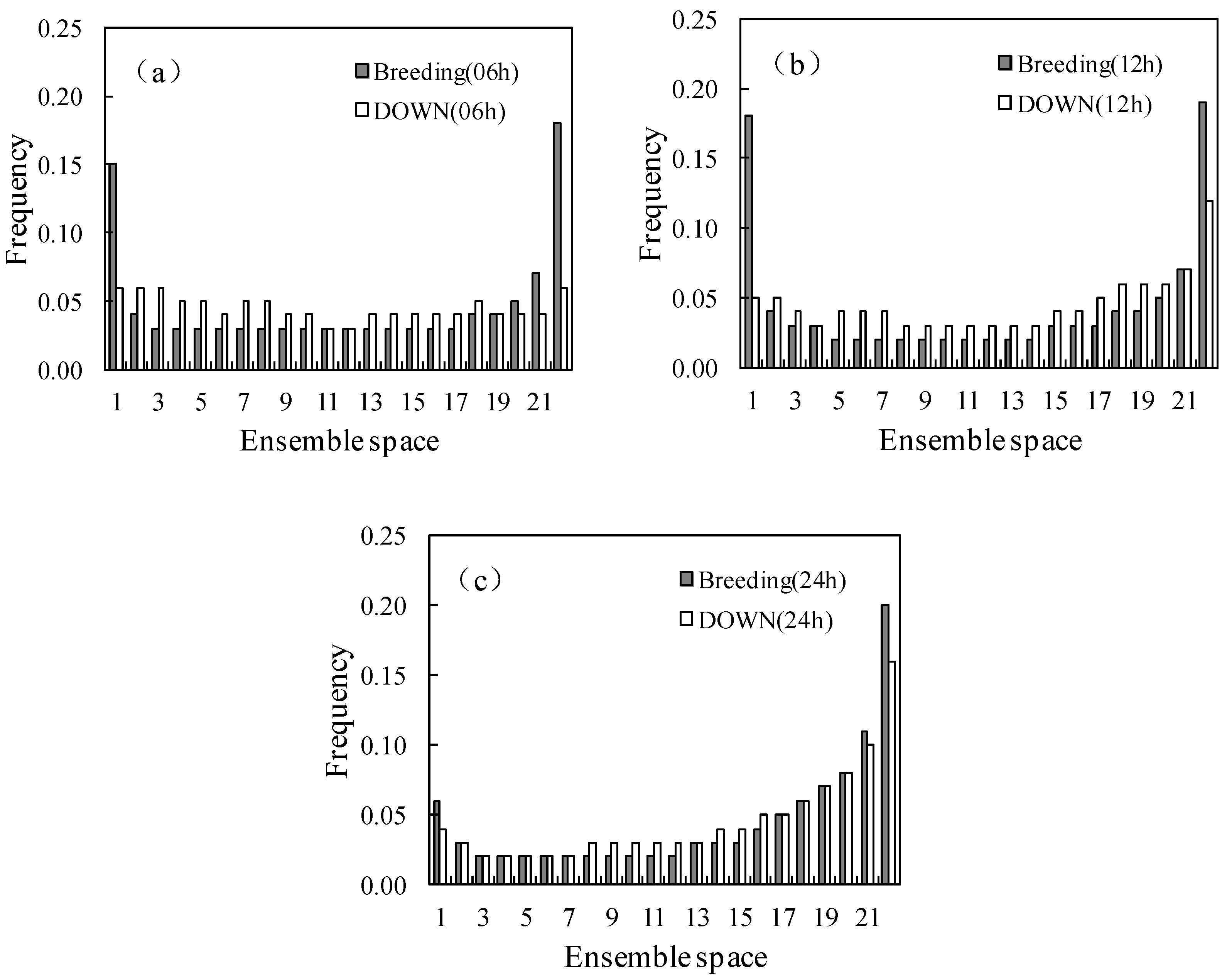
The statistical reliability of the two ensembles is shown in the Talagrand diagram. Figure 8 shows the Talagrand diagram for the zonal wind at 850 hPa and for the 6 h, 12 h and 24 h lead times. It is evident that for all graphs, the diagram of the Down ensemble is flatter than that of the Breeding ensemble; this result indicates that the frequency at which observations lie inside the entire Down ensemble is higher. Since both ensembles are underspread, a flatter Down ensemble pattern is desirable.
3.4. A Case Study
A typical heavy rainfall event that occurred in the summer of 2017 was studied. Both the Breeding and Down ensembles were initiated at 1200 UTC 21 May 2017.
Figure 9 shows the observed precipitation from 0000 UTC to 0006 UTC 22 May 2017, along with the heavy precipitation probability of the 6 h accumulated precipitation for both ensemble forecasts. As shown in the observation (Figure 9a), this case was characterized by a large precipitation area across North China, with the rainfall band exhibiting a northwest-southeast pattern and a maximum value greater than 25 mm. Figure 9b,c present the probability of the 6 h accumulated precipitation being greater than 13 mm. All the probability magnitudes are represented by shading. For the Down ensemble (Figure 9b), the area with magnitudes greater than 70% were located south of Beijing, and the high probability region (contoured) exhibited a southward shift relative to the observed precipitation center. For the Breeding ensemble (Figure 9c), the locations and ranges of the high probability areas were closer to the observations. For example, the range of probabilities higher than 70% near the southern part of Beijing was enlarged, and the area with a probability higher than 90% emerged at the border of Beijing and Tianjin, which corresponded well with the observation.
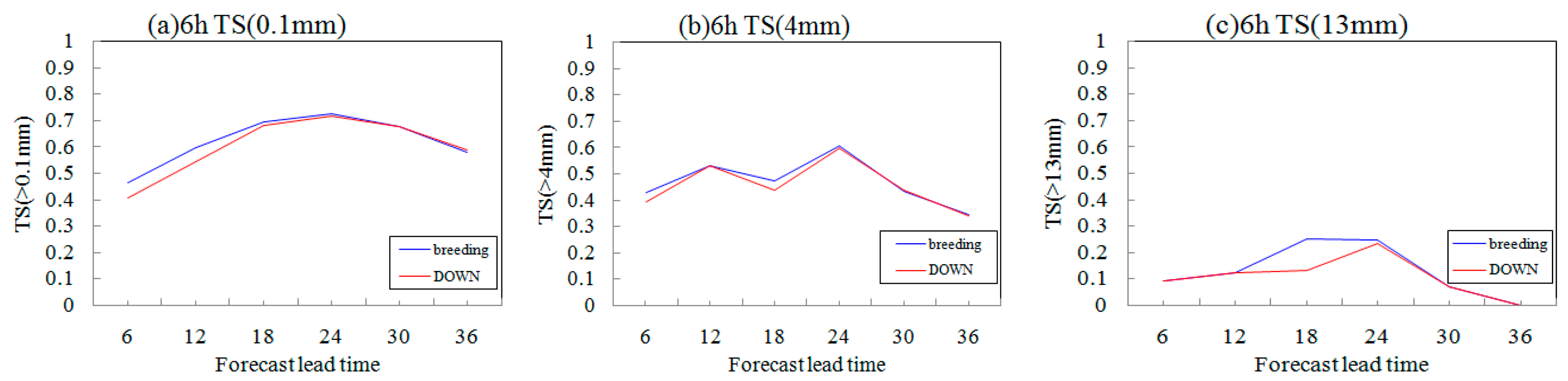
Figure 10 shows the TS of the 6 h accumulative precipitation for the ensemble mean forecast of both the Breeding scheme and Down scheme within a 36 h forecast period. For different magnitudes of the 6 h precipitation, the performance of the Breeding ensemble was better than that of the Down ensemble, and the advantage of the Breeding scheme was more notable within the short forecast lead times. Taking heavy rain (beyond the 13 mm threshold) as an example, the TS of the Breeding ensemble (0.25) exhibited a 50% improvement over that of the Down ensemble (0.13) for an 18 h forecast lead time.
The results presented above indicated that the Breeding method was superior to the downscaling method with regards to the location and magnitude of the precipitation forecasts. Thus, the Breeding method could provide a better reference than the downscaling method in operational precipitation forecasting.
In this section, the methods of Down and Breeding were compared in many respects. In summary, all the results are listed comprehensively in Table 1. It seemed that the Down method has a more widespread performance, which was more suitable for upper air variable forecasting, while the Breeding method seemed more appropriate for near-surface variable forecasting.
4. Summary and Conclusions
Based on the REPS of North China, comparative studies of two IC perturbation schemes for regional ensembles were conducted, namely, the Breeding and Down methods. Using the two IC perturbation schemes, consecutive ensemble forecast tests were conducted for a period of one month. The perturbation characteristics were investigated, and an ensemble verification was implemented using several probability forecast verification methods. Additionally, a heavy precipitation case was studied to examine the practical effectiveness of the two regional ensemble forecasting methods. In summary, the Breeding cycle-based perturbations and dynamical downscaling-based perturbations for the REPS had their own advantages and disadvantages, which are detailed as follows:
The perturbations generated by the Breeding method could provide high-resolution perturbation fields at the initial moment, including more abundant small-scale information, while the perturbations generated by the Down method contained more abundant large-scale perturbation information. With increasing forecast lead time, the differences between the Breeding and Down perturbations decreased at different scales. The two perturbation types showed different growth characteristics, primarily due to the different ways in which the perturbations were calculated. The Down perturbations came from the global ensemble, and therefore, the resolution of the Down perturbations was identical to that of the global model. When the perturbations were calculated using the Breeding method, the 12 h forecast perturbations from the previous REPS cycle were rescaled, and the perturbation scale would match the regional model resolution, thus exhibiting more abundant small-scale characteristics.
The perturbation growth of the Down method was faster than that of the Breeding method for short forecast lead times. For a long forecast lead time, the Breeding and Down schemes eventually became similar. This result indicated that the Down perturbations were better than the Breeding perturbations at evolving with the dynamic flow for short forecast lead times.
The one-month statistics of ensemble verifications were also revealing. The RMSE and spread verification showed that for upper air variables, the Down ensemble could obtain probabilistic forecast results that were improved over those of the Breeding scheme for short-range forecasting; the performance became very similar for long forecast lead times, while for near-surface variable forecasting, the forecasts of all members of the Breeding ensemble were more accurate.
A precipitation case study showed that the Breeding method was superior to the Down method with regard to the location and magnitude of precipitation forecasts. Thus, the Breeding method could provide an improved reference compared to the Down method for operational precipitation forecasting.
The results presented here indicated that although the performance of the Down perturbation ensemble was better than that of the Breeding perturbation ensemble in certain aspects, such as a more widespread growth and improved ensemble verification scores, the Breeding ensemble perturbations could better represent the forecast error of the regional model. Additionally, the Breeding method was more practical for near-surface variable forecasts. These comparisons may provide a reference for further improvement of the current REPS. A practical way to take advantage of both methods is to develop a blending technique, which has been investigated primarily by Caron [35] and Wang et al. [36] and blending techniques are expected to be appropriate methods in the future. For recent improvements, the Breeding method seems suitable.
Author Contributions
H.Z. conceived and designed the experiments. The paper was written by H.Z. with significant contributions from M.C. and S.F.
Funding
This work is financially supported by grants from the National Key R&D Program of China (grant no. 2018YFC1506804) and the National Natural Science Foundation of China (grant no. 41605082).
Acknowledgments
The authors thank the four reviewers for their constructive comments which benefit to improve the manuscript. This study was jointly funded by the National Key R&D Program of China (grant no. 2018YFC1506804) and the National Natural Science Foundation of China (grant no. 41605082).
Conflicts of Interest
The authors declare no conflicts of interest.
References
- Leith, C.E. Theoretical skill of Monte Carlo forecasts. Mon. Wea. Rev. 1974, 102, 409–418. [Google Scholar] [CrossRef]
- Toth, Z.; Kalnay, E. Ensemble forecasting at NMC: The generation of perturbations. Bull. Am. Meteor. Soc. 1993, 74, 2317–2330. [Google Scholar] [CrossRef]
- Molteni, F.; Buizza, R.; Palmer, T.N.; Petroliagis, T. The ECMWF ensemble prediction system: Methodology and validation. Quart. J. R. Meteor. Soc. 1996, 122, 73–119. [Google Scholar] [CrossRef]
- Houtekamer, P.L.; Lefaivrem, L.; Derome, J.; Ritchie, H.; Mitchell, H.L. A system simulation approachto ensemble prediction. Mon. Wea. Rev. 1996, 124, 1225–1242. [Google Scholar] [CrossRef]
- Buizza, R.; Houtekamer, P.L.; Toth, Z.; Pellerin, P.; Wei, M.; Zhu, Y. A comparison of the ECMWF, MSC and NCEP global ensemble prediction systems. Mon. Wea. Rev. 2005, 133, 1076–1097. [Google Scholar] [CrossRef]
- Wei, M.; Toth, Z.; Wobus, R.; Zhu, Y.; Bishop, C.H.; Wang, X. Ensemble Transform Kalman Filter-based ensemble perturbations in an operational global prediction system at NCEP. Tellus 2006, 58A, 28–44. [Google Scholar] [CrossRef]
- Marsigli, C.; Boccanera, F.; Montani, A.; Paccagnella, T. The COSMO-LEPS mesoscale ensemble system: Validation of the methodology and verification. Nonlinear Processes Geophys. 2005, 12, 527–536. [Google Scholar] [CrossRef]
- Frogner, I.L.; Haakenstad, H.; Iversen, T. Limited-area ensemble predictions at the Norwegian Meteorological Institute. Quart. J. R. Meteor. Soc. 2006, 132, 2785–2808. [Google Scholar] [CrossRef] [Green Version]
- Bouttier, F.; Raynaud, L.; Nuissier, O.; Ménétrier, B. Sensitivity of the AROME ensemble to initial and surface perturbations during HyMeX. Q. J. R. Meteorol. Soc. 2016, 142, 390–403. [Google Scholar] [CrossRef]
- Bowler, N.E.; Arribas, A.; Mylne, K.R.; Robertson, K.B.; Beare, S.E. The MOGREPS short-range ensemble prediction system. Quart. J. R. Meteor. Soc. 2008, 134, 703–722. [Google Scholar] [CrossRef] [Green Version]
- Clark, A.J.; Gallus, W.A.; Xue, M.; Kong, F.Y. Convection-Allowing and Convection-Parameterizing Ensemble Forecasts of a Mesoscale Convective Vortex and Associated Severe Weather Environment. Wea. Forecasting. 2010, 25, 1052–1081. [Google Scholar] [CrossRef] [Green Version]
- Hohenegger, C.; Walser, A.; Langhans, W.; Schär, C. Cloud-resolving ensemble simulations of the August 2005 Alpine flood. Quart. J. R. Meteor. Soc. 2008, 134, 889–904. [Google Scholar] [CrossRef]
- Kuhnlein, C.; Keil, C.; Craig, G.C.; Gebhardt, C. The impact of downscaled initial condition perturbations on convection-allowing ensemble forecasts of precipitation. Q. J. R. Meteorol. Soc. 2014, 140, 1552–1562. [Google Scholar] [CrossRef]
- Peralta, C.; ben Bouallegue, Z.; Theis, S.E.; Gebhardt, C.; Buchhold, M. Accounting for initial condition uncertainties in COSMO-DE-EPS. J. Geophys. Res. 2012, 117, 1–13. [Google Scholar] [CrossRef]
- Wang, Y.; Bellus, M.; Wittmann, C.; Steinheimer, M.; Weidle, F.; Kann, A.; Ivatek-Šahdan, S.; Tian, W.; Ma, X.; Tascu, S.; et al. The Central European limited area ensemble forecasting system: ALADIN-LAEF. Quart. J. R. Meteor. Soc. 2011, 134, 483–502. [Google Scholar] [CrossRef]
- Toth, Z.; Kalnay, E. Ensemble forecasting at NCEP and the Breeding method. Mon. Wea. Rev. 1997, 125, 3297–3319. [Google Scholar] [CrossRef]
- Buizza, R.; Palmer, T.N. The Singular-Vector Structure of the Atmospheric Global Circulation. J. Atmos. Sci. 1995, 52, 1434–1456. [Google Scholar] [CrossRef] [Green Version]
- Wang, X.; Bishop, C.H. A comparison of Breeding and ensemble transform Kalman filter ensemble forecast schemes. J. Atmos. Sci. 2003, 60, 1140–1158. [Google Scholar] [CrossRef]
- Stensrud, D.J.; Brooks, H.E.; Du, J.; Tracton, M.S.; Rogers, E. Using ensembles for short-range forecasting. Mon. Wea. Rev. 1999, 127, 433–446. [Google Scholar] [CrossRef]
- Du, J.; DiMego, G.; Tracton, M.S.; Zhou, B. NCEP short range ensemble forecasting (SREF) system: Multi-IC, multi-model and multi-physics approach. CAS/JSC WGNE Res. Act. Atmos. Ocea. Modell. 2003, 33, 5.09–5.10. [Google Scholar]
- Li, X.; Charron, M.; Spacek, L.; Candille, G. A regional ensemble prediction system based on moist targeted singular vectors and stochastic parameter perturbations. Mon. Wea. Rev. 2008, 136, 443–462. [Google Scholar] [CrossRef]
- Zhang, H.; Chen, J.; Zhi, X.; Li, Y.; Sun, Y. Study on the Application of GRAPES Regional Ensemble Prediction system. Meteorol. Mon. 2014, 40, 1077–1088. [Google Scholar]
- Bowler, N.E.; Mylne, K.R. Ensemble transform Kalman filter perturbations for a regional ensemble prediction system. Quart. J. R. Meteor. Soc. 2009, 135, 757–766. [Google Scholar] [CrossRef] [Green Version]
- Saito, K.; Hara, M.; Seko, H.; Kunii, M.; Yamaguchi, M. Comparison of initial perturbation methods for the mesoscale ensemble prediction system of the Meteorological Research Institute for the WWRP Beijing 2008 Olympics Research and Development Project (B08RDP). Tellus 2011, 63, 445–467. [Google Scholar] [CrossRef] [Green Version]
- Zhang, H.; Chen, J.; Zhi, X.; Wang, Y. A Comparison of ETKF and Downscaling in a Regional Ensemble Prediction System. Atmosphere 2015, 6, 341–360. [Google Scholar] [CrossRef] [Green Version]
- Zhang, H.; Li, Y.; Fan, S.; Zhong, J.; Lu, B. Study on initial perturbation construction method for regional ensemble forecast based on dynamical downscaling. Meteorol. Mon. 2017, 43, 1461–1472. [Google Scholar]
- Skamarock, W.C.; Klemp, J.B.; Dudhia, J.; Gill, D.O.; Barker, D.M.; Duda, M.G.; Huang, X.Y.; Wang, W.; Powers, J.G. A Description of the Advanced Research WRF Version 3; NCAR Technical Note NCAR/TN–475STR; National Center for Atmospheric Research: Boulder, CO, USA, 2008. [Google Scholar]
- Pilguj, N.; Czernecki, B.; Kryza, M.; Migała, K.; Kolendowicz, L. Application of the Polar WRF model for Svalbard—sensitivity to planetary boundary layer, radiation and microphysics schemes. Polish Polar Res. 2018, 39, 349–370. [Google Scholar]
- Weichert, A.; Burger, G. Linear versus nonlinear techniques in downscaling. Clim. Res. 1998, 10, 83–93. [Google Scholar] [CrossRef] [Green Version]
- Cannon, A.J.; Whitfield, P.H. Downscaling recent stream-flow conditions in British Columbia, Canada using ensemble neural networks. J. Hydro. 2002, 259, 136–151. [Google Scholar] [CrossRef]
- Palmer, T.N.; Gelaro, R.; Barkmeijer, J.; Buizza, R. Singular vectors, metrics, and adaptive observations. J. Atmos. Sci. 1998, 55, 633–653. [Google Scholar] [CrossRef]
- Hamill, T.M. Interpretation of rank histograms for verifying ensembles. Mon. Wea. Rev. 2001, 129, 550–560. [Google Scholar] [CrossRef]
- Gilbert, G.K. Finley’s tornado predictions. Amer. Meteor. J. 1884, 1, 166–172. [Google Scholar]
- Denis, B.; Cote, J.; Laprise, R. Spectral decomposition of two-dimensional atmospheric fields on limited-area domainsusing discrete cosine transform (DCT). Mon. Wea. Rev. 2002, 130, 1812–1829. [Google Scholar] [CrossRef]
- Caron, J.F. Mismatching Perturbations at the Lateral Boundaries in Limited-Area Ensemble Forecasting: A Case Study. Mon. Wea. Rev. 2013, 141, 356–374. [Google Scholar] [CrossRef]
- Wang, Y.; Bellus, M.; Geleyn, J.F.; Ma, X.; Tian, W.; Weidle, F. A New Method for Generating Initial Condition Perturbations in a Regional Ensemble Prediction System: Blending. Mon. Wea. Rev. 2014, 142, 2043–2059. [Google Scholar] [CrossRef]
Figure 1.
The model domain configuration for the North China REPS.

Figure 2.
Flow chart of the REPS Breeding cycle.

Figure 3.
Member-averaged power spectra of the 500 hPa zonal wind perturbations as a function of wavelength for Down and Breeding. (a) Down and (b) Breeding.
Figure 3.
Member-averaged power spectra of the 500 hPa zonal wind perturbations as a function of wavelength for Down and Breeding. (a) Down and (b) Breeding.

Figure 4.
Vertical distributions of the zonal wind perturbation (unit: m·s−1); the different lines denote different forecast lead times. (a) Down; (b) Breeding; and (c) Down minus Breeding.
Figure 4.
Vertical distributions of the zonal wind perturbation (unit: m·s−1); the different lines denote different forecast lead times. (a) Down; (b) Breeding; and (c) Down minus Breeding.

Figure 5.
Horizontal spread of the zonal wind (unit: m·s−1) at different forecast lead times for the Breeding and Down ensembles. (a) Down 00 h; (b) Down 12 h; (c) Down 24 h; (d) Breeding 00 h; (e) Breeding 12 h; and (f) Breeding 24 h.
Figure 5.
Horizontal spread of the zonal wind (unit: m·s−1) at different forecast lead times for the Breeding and Down ensembles. (a) Down 00 h; (b) Down 12 h; (c) Down 24 h; (d) Breeding 00 h; (e) Breeding 12 h; and (f) Breeding 24 h.

Figure 6.
RMSE of the ensemble mean, ensemble spread and their ratio as a function of the forecast lead time for the Breeding and Down schemes. (a) RMSE and spread for T500; (b) RMSE and spread for U500; (c) ratio of the spread and RMSE for T850; and (d) ratio of the spread and RMSE for U850.
Figure 6.
RMSE of the ensemble mean, ensemble spread and their ratio as a function of the forecast lead time for the Breeding and Down schemes. (a) RMSE and spread for T500; (b) RMSE and spread for U500; (c) ratio of the spread and RMSE for T850; and (d) ratio of the spread and RMSE for U850.

Figure 7.
Box plot of the 2 m temperature forecast at a Beijing station for the two schemes. (a) Down and (b) Breeding.
Figure 7.
Box plot of the 2 m temperature forecast at a Beijing station for the two schemes. (a) Down and (b) Breeding.

Figure 8.
Talagrand diagram of the 850 hPa zonal wind forecast for the Breeding and Down schemes. (a) 6 h forecast; (b) 12 h forecast; and (c) 24 h forecast.
Figure 8.
Talagrand diagram of the 850 hPa zonal wind forecast for the Breeding and Down schemes. (a) 6 h forecast; (b) 12 h forecast; and (c) 24 h forecast.

Figure 9.
Observational state and heavy precipitation probability of the 6 h accumulative precipitation: (a) observation (units: mm); (b) precipitation probability of being greater than 13 mm (units: %) for the Down ensemble forecast; and (c) as in (b) but for the Breeding forecast.
Figure 9.
Observational state and heavy precipitation probability of the 6 h accumulative precipitation: (a) observation (units: mm); (b) precipitation probability of being greater than 13 mm (units: %) for the Down ensemble forecast; and (c) as in (b) but for the Breeding forecast.

Figure 10.
Threat score of the ensemble mean forecast 6 h accumulative precipitation for the Breeding ensemble and Down ensemble: (a) greater than 0.1 mm; (b) greater than 4 mm; and (c) greater than 13 mm.
Figure 10.
Threat score of the ensemble mean forecast 6 h accumulative precipitation for the Breeding ensemble and Down ensemble: (a) greater than 0.1 mm; (b) greater than 4 mm; and (c) greater than 13 mm.


Table 1.
Summary of the comparison of both ensembles for all aspects.
| Aspect | Performance |
|---|---|
| Perturbation scale | Breeding is better at generating more small-scale perturbations at the initial time |
| Perturbation growth | Down shows better growth for short range forecasts |
| Upper air verification | Down is more widespread and has a smaller RMSE for short range forecasts |
| Near-surface verification | Breeding is more precise and reliable |
| Precipitation forecast | Breeding has a better performance |
© 2019 by the authors. Licensee MDPI, Basel, Switzerland. This article is an open access article distributed under the terms and conditions of the Creative Commons Attribution (CC BY) license (http://creativecommons.org/licenses/by/4.0/).
Share and Cite
MDPI and ACS Style
Zhang, H.; Chen, M.; Fan, S. Study on the Construction of Initial Condition Perturbations for the Regional Ensemble Prediction System of North China. Atmosphere 2019, 10, 87. https://doi.org/10.3390/atmos10020087
AMA Style
Zhang H, Chen M, Fan S. Study on the Construction of Initial Condition Perturbations for the Regional Ensemble Prediction System of North China. Atmosphere. 2019; 10(2):87. https://doi.org/10.3390/atmos10020087
Chicago/Turabian StyleZhang, Hanbin, Min Chen, and Shuiyong Fan. 2019. "Study on the Construction of Initial Condition Perturbations for the Regional Ensemble Prediction System of North China" Atmosphere 10, no. 2: 87. https://doi.org/10.3390/atmos10020087
Note that from the first issue of 2016, this journal uses article numbers instead of page numbers. See further details here.