Recurrence Spectra of European Temperature in Historical Climate Simulations


1
Laboratoire des Sciences du Climat et de l’ Environnement, UMR 8212 CEA-CNRS-UVSQ, IPSL, Université Paris-Saclay, F-91191 Gif-sur-Yvette, France
2
Climate Simulation and Prediction Division, Centro Euro-Mediterraneo sui Cambiamenti Climatici, CMCC, Viale Berti Pichat, 6/2, 40127 Bologna, Italy
3
London Mathematical Laboratory, 8 Margravine Gardens, London W6 8RH, UK
4
The Climate Data Factory, 12 Rue de Belzunce, 75010 Paris, France
*
Author to whom correspondence should be addressed.
Atmosphere 2019, 10(4), 166; https://doi.org/10.3390/atmos10040166
Submission received: 16 January 2019
/
Revised: 22 March 2019
/
Accepted: 23 March 2019
/
Published: 28 March 2019
(This article belongs to the Special Issue Weather and Climate Extremes: Current Developments)
Abstract
:We analyse and quantify the recurrences of European temperature extremes using 32 historical simulations (1900–1999) of the fifth Coupled Model Intercomparison Project (CMIP5) and 8 historical simulations (1971–2005) from the EUROCORDEX experiment. We compare the former simulations to the 20th Century Reanalysis (20CRv2c) dataset to compute recurrence spectra of temperature in Europe. We find that, (1) the spectra obtained by the model ensemble mean are generally consistent with those of 20CR; (2) spectra biases have a strong regional dependence; (3) the resolution does not change the order of magnitude of spectral biases between models and reanalysis, (4) the spread in recurrence biases is larger for cold extremes. Our analysis of biases provides a new way of selecting a subset of the CMIP5 ensemble to obtain an optimal estimate of temperature recurrences for a range of time-scales.
1. Introduction
Climate events linked to extremes of temperature (heatwaves/cold spells) [1,2,3] have severe impacts on human health and natural ecosystems [4,5,6]. Heatwave events have increased in Europe within the last decades in frequency or intensity, while cold spells have decreased in frequency and intensity since 1950 [7,8,9,10,11]. An important question to evaluate the future evolution of such events is whether climate models are able to reproduce temperature distributions and their extremes.
Several studies already have focused on this issue [12,13,14,15,16,17,18]. Most of them show substantial inconsistencies between observed and modeled temperature distributions. Morak et al. [16] uses the Hadley Centre Global Environmental Model, version 1 (HadGEM1) with both anthropogenic and natural forcings to demonstrate that although the model shows a tendency to significantly overestimated changes in warm extremes, changes in temperature extremes are generally well captured by the model. In the latest version, HadGEM3-A [19], models overestimated warm extremes especially in central/northern Europe while cold extremes appear well simulated. Thus, one of the most striking findings in [19] is the ability of the model to capture and reproduce the main observed North-Atlantic atmospheric weather regimes responsible for temperature and precipitation extreme events.
Regarding Coupled Model Intercomparison Project (CMIP) models, Sillmann et al. [18] shows that the spread amongst CMIP5 models for several temperature indices (including extremes) is reduced compared to CMIP3 models demonstrating, as well, that the median model climatology outperforms individual models for all indices. In Krueger et al. [15] a comparison of weather patterns from CMIP5 models with patterns derived from ERA interim indicates that climate models simulate mechanisms associated with temperature extremes reasonably well, in particular circulation-based mechanisms. More recently, Li et al. [20] find that climate models forced with natural and anthropogenic historical forcings underestimate changes in temperature extremes. Conversely, other studies e.g., Kharin et al. [21] have found that climate models provide a good estimation for warm temperature extremes but poor estimations of cold extremes, especially in sea ice covered areas.
Most of those analyses focus on extremely low or high temperature values, and model those extremes with Generalized Extreme Value (GEV) distributions [22,23,24]. Studies focusing on climate variability have investigated the Fourier spectra of temperature from observations and climate model simulations. Such studies have emphasized the role of periodic or quasi-periodic features of the climate system [25].
The present paper combines the paradigms of Fourier spectra and extreme events, by focusing on the range of return levels associated with return period for rare temperature events. Thus we want to assess the whole spectrum of probabilities of events linked to temperature, and investigate how climate models simulate rare temperature events. In this approach, we estimate the recurrences for points of the phase space of the underlying dynamical system, by computing probabilities of events. Those probabilities have known GEV asymptotic distributions [26,27] that can be used to check the reliability and robustness of estimated return levels. The recent study of Faranda et al. [28] shows that the recurrence method can be adapted to the study of atmospheric variables even when the underlying exact dynamics of the system (in terms of dynamical systems) is unknown. In [28] rare recurrences are computed using different approaches (Recurrences and Block maxima) and comparing the IPSL-CM5 historical model within the CMIP5 historical experiment with two long-terms reanalyses (ERA20C and 20CR). Their results show that with respect to the traditional approaches, the recurrence technique is sensitive to the change in the size of the selection window of extremes due to the conditions imposed by the dynamics.
In this paper we investigate the recurrence properties of temperature values in ensembles of climate model simulations, using the technique developed in Faranda and Vaienti [29]. This allows quantifying the properties of rare values of the system, by accounting for its chaotic nature.To perform our analysis, we use the multi-model ensemble of coupled ocean-atmosphere General Circulation Models (GCMs) provided by the Coupled Model Intercomparison Project Phase 5 (CMIP5) [30]. The main goal of our analysis is to evaluate how CMIP5 model simulations covering 1900–1999 can represent the recurrences in extremes events using a dynamical system technique developed by Faranda et al. [28] and to further investigate the existence of biases among models and observations. In order to assess the dependence of the results on the horizontal resolution, we also use the bias Corrected EURO-CORDEX Climate Projections for the period 1971–2005.
This paper is organized as follows: first, we present the data sets (models and observations), the region of our study and we describe our analysis method, then, we compute and analyze temperature return levels and compare them to the 20th Century Reanalysis 20CRv2c dataset. Finally we discuss and summarize the main results.
2. Data
We base our analysis on daily 2-m temperature (t2m) from the historical experiment (1900–1999) of the Coupled Model Intercomparison Project Phase 5 (CMIP5) [30]. CMIP5 daily model output is available for 32 models for the historical experiment. The rationale of the CMIP5 ensemble is that it samples a large fraction of the possible climate states that are compatible with observed natural and anthropogenic forcings, rather than one trajectory (i.e., the observations). In order to compute the return levels, we compare those 32 models (Table 1) with the 20th Century Reanalysis data version 2c (20CRv2c, [31]). We have selected 20CRv2c in this study because it is the latest version of 20CR and has bias correction applied to the sea-ice distribution by assimilating new SST and sea-ice cover (SIC) data [32]. However, we have found similar results (not shown here), with slight differences for some models, when we have tested other reanalysis (ERA20C and former 20CR, results for IPSL in [28]). We consider the ensemble mean of the 56 realizations of 20CR, as is usually done in the literature. Alvarez-Castro et al. [7] analyzed the whole ensemble members for European heatwaves and argued that the ensemble mean provides robust features of the dynamical properties. The analysis is focused on the European region, between N– N and W–32 E. The horizontal resolution of 20CR is 2 and for a better comparison, all the datasets have been bilinearly re-interpolated onto the 20CRv2c grid. Models are sorted in tables and figures by decreasing resolution.
We compute then the Ensemble Model Mean (EMM) and the standard deviation of the model ensemble (SDM), since these are synthetic useful indicators to evaluate the models spread. Then, we confront the EMM to the ensemble mean of 20CRv2c (ensemble composed of 56 members). To complete our study, we analyse the outputs of 8 post-processed (Table 2) regional models simulations from the bias Corrected EURO-CORDEX Climate Projections for the period 1971–2005. The EURO-CORDEX initiative is a part of the global Coordinated Regional Downscaling Experiment (CORDEX, http://wcrp-cordex.ipsl.jussieu.fr/) to improve regional climate scenarios for the land-regions worldwide. It provides regional climate projections for Europe at 50 km and 12.5 km resolution, which downscale the CMIP5 global climate projections and the RCP scenarios (See [33,34] for further information). The bias correction methodology uses the general Cumulative Distribution Function transform method (CDFt) of [35]. It assumes a reference period over which observation-based data is available: 1971–2005. The reference dataset is the 0.22-rotated E-OBS version 10 data set [36] that can be downloaded from http://eca.knmi.nl.
3. Methods
We assume that the climate variables have trajectories that wind around a chaotic attractor that contains the underlying dynamics of the system. We fix an arbitrary temperature and we consider the probability that the time series returns within a tolerance to . The return period is defined as the average time it takes for the time series to "hit" this interval. More precisely, the recurrence technique computes the probability Pr that the variable T returns in an interval of radius centered in : .
Following [29], we provide the algorithm for defining the spectrum of recurrences for temperature time series:
- Compute the observable
- Divide the series into n bins each containing m data and extract the maxima , with .
- Distribution functions like are modelled, for n sufficiently large, by the so-called generalized extreme value (GEV) distribution which depend on three parameters and such that:The parameter is called the tail index; when its value is the GEV corresponds to the Gumbel type of distribution. Indeed this is the expected distributions of recurrences, providing that we use the observable.
- Perform an Anderson and Darling [37] test to assess whether the fit is compatible with a Gumbel distribution.
If the fit is found to be compatible with a Gumbel distribution, one can repeat the procedure for shorter bin lengths and find the smallest m such that, for the chosen , the fit converges. This defines the shortest convergent recurrence time and its corresponding return value ℓ. Note that, not for all the it is possible to find a value of m such that the fit to the Gumbel law is acceptable. The range of values such that there is a suitable m defines the spectrum of recurrences as illustrated in Figure 1. Rare temperatures are located in the white area between the red lines and the blue area. This provides an alternative definition of maximum and minimum temperatures based on the rarity of the recurrences. In the following we will stick this definition to define temperature hot and cold extremes. This representation of a recurrence spectrum (i.e., temperature levels as a function of return times) is analogous to a Fourier spectrum (i.e., temperature values as a function of frequency), but for nonperiodic phenomena.
We consider 100 years (1900–1999) of daily temperature data for the whole year. This allows testing return times m between 6 months up to 4 years [28]. For recurrence windows longer than 4 years, we get less than 25 years of temperature recurrences and unreliable estimates of the Gumbel distributions. Conversely, events chosen for bin lengths shorter than 6 months cannot be considered as rare. We are dealing with non-stationary time series. However, the values of ℓ in the spectra are not on the tails of the distribution of which implied that the non-stationarity (about 0.5 C/century) does not affect the convergence to the spectrum.
The procedure as well as the parameters used in this study is the same as in Faranda et al. [28].
4. Results
We evaluate how CMIP5 historical simulations can represent the recurrences in extremes events using the methodology of [28] to further illustrate the biases between CMIP5 models and a reference (20CRv2c). Here the term bias refers to the difference between CMIP5 and 20CRv2c recurrence spectra.
4.1. Changes in European Temperature Recurrence Spectrum
We illustrate the capabilities of the method by showing the results for three specific locations over Europe (Figure 2). Here the curves represent the spectrum for a grid point in central Europe (a), northern Europe (b) and southern Europe (c). The different shapes of the red lines (20CR), describing the area of normal recurrences, are explainable in terms of the climate characteristics of the grid points considered. Central Europe (a) features a continental climate with very cold extremes of temperature, being C rare for a return time of 1 year while C becomes normal for higher return times. From 1 to 4 years of return times, C are normal temperature in warm extremes. The grid point of Northern Europe (b) is located close to the Baltic sea showing mild temperatures in comparison with a more continental Northern point. Even though, the shape of red line shows cold extremes of temperature reach C for normal recurrences in return times of 2–4 years and 20 C for warm extremes in return times of 1–4 years. Temperatures lower than C are rare for return time of 1 year or less. Southern Europe grid point is located in Guadalquivir valley, presenting very hot extremes of temperatures reaching 40 C as normal recurrences from 1 to 4 years of return times. Cold extremes instead are rare for temperatures lower than 0 C. All the models show that return levels for hot temperature extremes are similar for years (Figure 2). The EMM and the SDM shows similar behavior with ℓ almost constant for years.
However, return levels for the cold temperature extremes do depend on the bin length. For cold (hot) temperature extremes the disagreement (agreement) between the models increases (decreases) with the bin length, () and differences between 20CRv2c and EMM also increase (decrease) with the bin length ().
The agreement between return levels for models and the 20CR (Figure 2) depends on the location. For location (a), the matching between EMM and 20CRv2c is good for both the hot and the cold temperature extremes. Only few models deviate significantly from the reanalysis. For location (b) the representation of cold and warm extremes is poor both for single models and EMM. Even if there is inconsistency among each single model and 20CRv2c, the EMM follows the behavior of the reanalysis but it underestimates the hot and overestimates the cold temperature extremes. In location (c), models are more coherent, although the EMM is shifted towards colder extremes for both the hot and the cold temperature extremes.
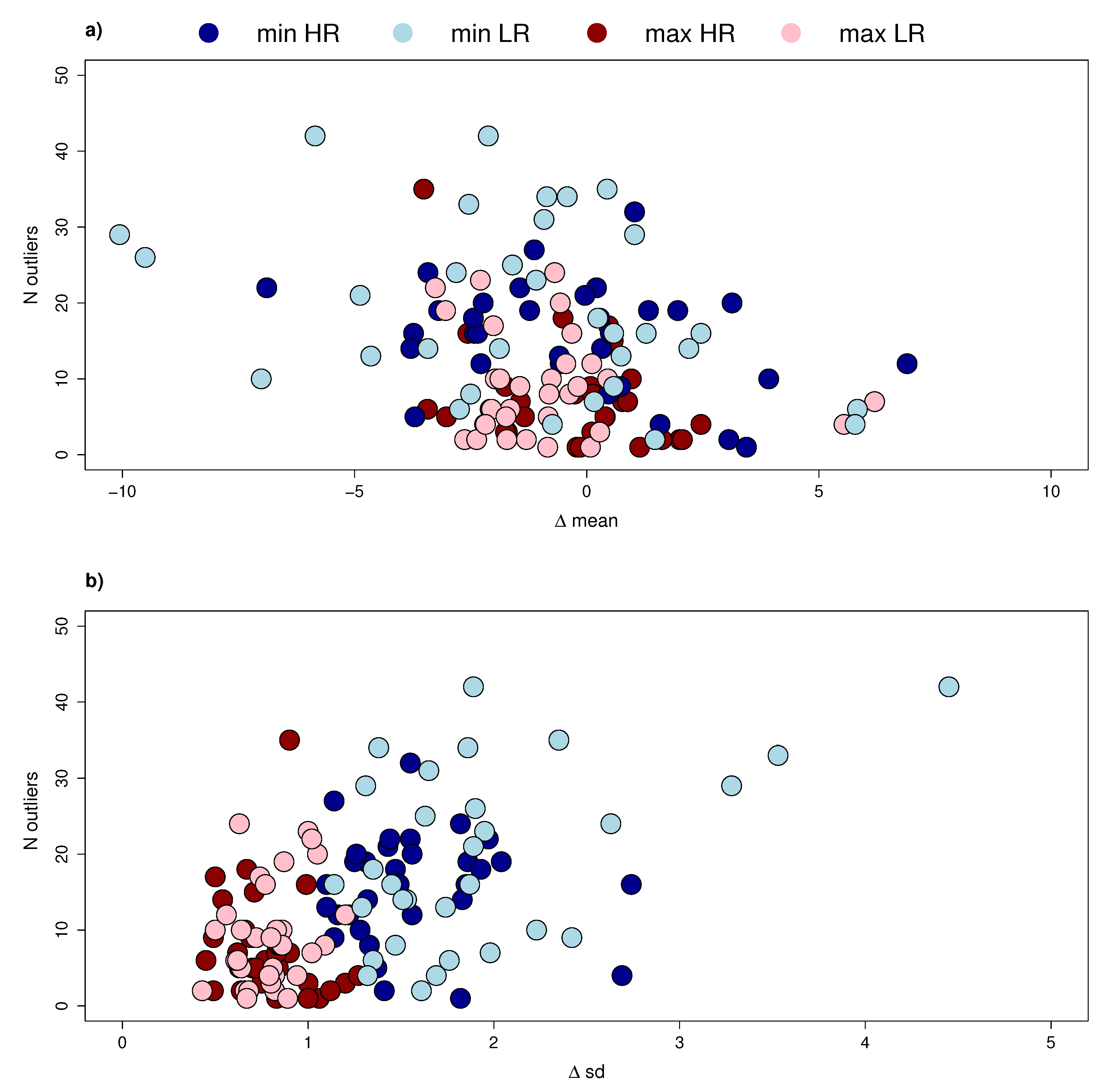
The distribution of the biases in return levels at all grid points is provided in Figure 3 in blue for the cold and red for the hot temperature extremes. Numbers correspond to CMIP5 models in Table 1, sorted by decreasing in resolution in order to investigate the role of horizontal resolution. Figure 3 illustrates the probability distribution of biases between models and 20CRv2c showing the results for 1 year (Panels a and c) and 4 years (Panels b and d) bin lengths m. Table 3 contains the statistical information in Figure 3. The boxplots demonstrate the results obtained at some specific location (Figure 2): the cold extremes show larger biases than the hot extremes. This premise is also evident in Figure 4 and Figure 5. Figure 4 shows the errorbars of the biases in cold extremes (a) and hot extremes (b) for all the bin lengths m. Moreover, biases in warm extremes do not change significantly with the bin length. A Kolmogorov-Smirnov test shows that the distribution of biases is neither Gaussian nor centered around zero for the models and the ensemble (Figure 5). The number of outliers in Figure 5 is represented vs the mean of the biases (a) and the standard deviation (b) for and by model (Higher/lower resolution in dark/light colours). In most cases, there are many outliers, despite the fact that the standard deviation of the biases (Figure 4) is relatively small (Table 3). The ideal case is only found for the hot temperature extremes at years of the MIROC5 model. This analysis shows that biases are not linked to the low/high resolution of the GCMs since there is no trend in Figure 3, Figure 4 and Figure 5.
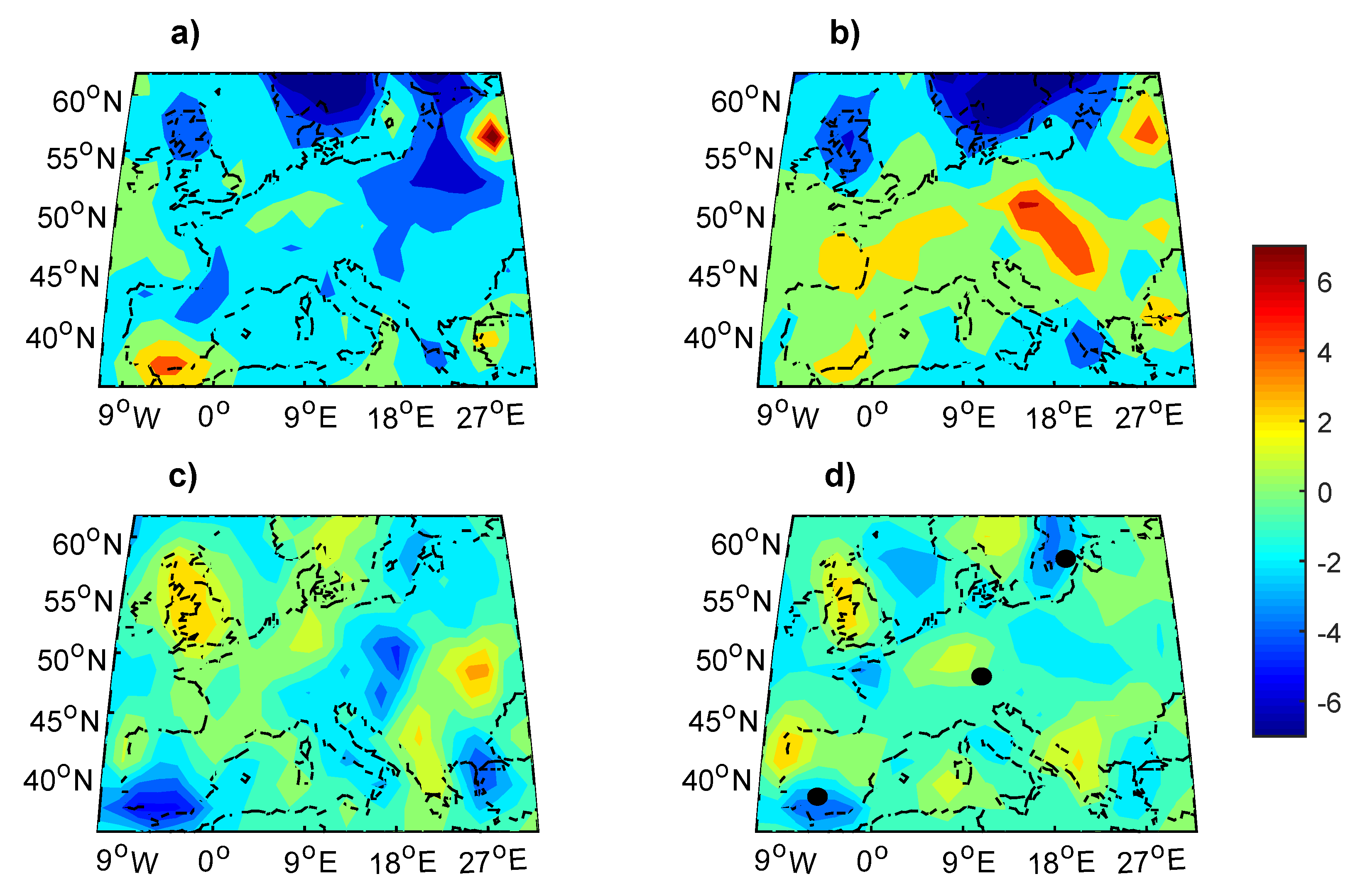
We focus now on the spatial distribution of biases in order to investigate their coherence. We concentrate on two quantities: the average biases of models EMM, obtained as the difference between the ensemble mean and 20CR return levels at each grid point (Figure 6), and the SDM at each grid point (Figure 7). Following the same structure of Figure 3, Figure 4 and Figure 5 and the cold extremes (Figure 6a,b) show larger deviations than the hot extremes (Figure 6c,d). This analysis shows the geographical distribution of biases: for the cold extremes, the Southwestern Iberian peninsula shows the largest positive biases, while for the largest negative biases occur in the Scandinavian region. The SDM (Figure 7) shows a coherent spatial structure for both the cold extremes (a, b) and the hot extremes (c, d). For the cold temperatures, larger biases appear mostly in the Scandinavian peninsula. For hot temperatures, biases are in general small for both and year, except at some specific grid points where they are mainly concentrated over the Baltic sea.
4.2. Effects of Resolution: A Regional Application
The sole use of CMIP5 simulations is not conclusive on the dependence on the resolution of temperature extremes biases. Indeed the simulations span only a limited range of scale of order of hundreds kilometers. To complete this study, we therefore analyze the outputs of 8 post-processed regional models simulations (Table 2) from the bias Corrected EURO-CORDEX Climate Projections for the period 1971–2005. Regional climate models add crucial spatial detail for temperature extremes, allowing us to study fine-scale processes missing in Global Circulation Models,(e.g., Urban effects). As for CMIP5 models, for the regional simulations we compute the EMM and SDM in a similar way. These results are displayed in Figure 8. They show that increasing the resolution does not reduce the order of magnitude of the SDM. As in the CMIP5 case, biases for the hot temperature extremes are smaller than for the cold temperature extremes. The hot extremes biases are mostly located on the Iberian Peninsula, as for CMIP5 models. The cold biases appear anywhere in continental Europe and do seem not directly linked to the orography. These results are in line with Vautard, et al. [34] and Lhotka and Kysely [38]. In Vautard, et al. [34] most of the regional models show an overestimation of hot temperature extremes in Mediterranean regions and an underestimation over Scandinavia. Thus, a preliminary analysis of the sources of spread show that the simulation of hot temperature is primarily sensitive to the convection and the microphysics schemes. Lhotka and Kysely [38] suggest that simulated cold events in central Europe should be analyzed and interpreted with caution, since they may develop also under zonal flow in some models, which contradicts observations.
5. Discussion
We have analyzed the recurrence spectra for hot and cold temperature values in the European region by using a methodology that provides robust estimates of return levels. In order to assess the dependence on the horizontal resolution on the temperature extremes biases, we have used both CMIP5 global medium resolution simulations and regional high resolutions runs from EURO-CORDEX.
Our results show that inconsistencies of European recurrence spectra between models and reanalysis can be much larger than the climate change signal in each model. Moreover, although the biases are generally centered around zero, their spatial variability suggests that these are caused not only by the differences in the average temperature of CMIP5 models but they largely depends on model dynamics/physics. For cold temperatures we find that biases depend on the chosen return period, whereas for the hot temperatures this dependence is observed only for return periods shorter than the seasonal cycle. An additional important difference is that, while for warm temperatures the biases are centered around zeros, for rare () cold temperatures the average biases are mostly positive, although bias model dependence is very large. In individual models, the asymmetry between hot and cold temperature recurrences and their biases is probably due to the (mis)representation of the albedo for negative temperatures, as already discussed by [39]. Indeed an ensemble average of CMIP5 simulations allows to reduce those biases even though the distributions of hot and cold temperature extremes differ in variance and number of outliers with respect to the 20CRv2c reanalysis.
Our results suggest how to perform models selection in order to avoid the models leading to biased estimations of temperatures extremes on extended regions as well as on specific grid-points for both global (CMIP5) and regional (EURO-CORDEX) simulations. This outcome is coherent with Tebaldi and Knutti [40] who argued that the quantification of all aspects of model biases requires multi-model ensembles, ideally as a complement to the exploration of single-model bias.
Our analysis gives geographical details on the distribution of the biases: in general we find that models have the largest biases in hot temperature values in South Western Europe for both global and regional simulations. For CMIP5 simulations, cold temperature extremes biases are larger over North Europe and the multi-model bias spread is larger on the coastal grid-points. Improving the resolution does not change the order of magnitude of the averaged biases although the multi-model spread is reduced on the coasts. Overall, the biases in temperature extremes for recurrences in EURO-CORDEX simulations seem to be related to the physical parameterizations instead of the orography, since some areas with complex geography do not present large biases. This motivates to further pursue the bias corrections techniques to include the physical mechanisms at the origin of the biases in cold temperature extremes, e.g., water phase transitions or ice-radiation feedbacks and interactions.
6. Conclusions
This paper presents a tool for a general assessment of biases in the recurrence spectra for temperatures. We find that:
- The recurrence spectra obtained by the model ensemble mean are generally consistent with those of 20CRv2c.
- The spectra biases have a strong regional dependence.
- A comparison with an ensemble of regional climate simulations shows that the resolution does not change the order of magnitude of spectral biases between models and reanalysis.
- The spread in recurrence biases is larger for cold extremes.
Our analysis of biases provides a new way of selecting a subset of the CMIP5 ensemble to obtain an optimal estimate of temperature recurrences for a range of time-scales. This assessment could be extended to investigate the seasonal dependence of such the spectra, or their dependence on future climate change.
In a changing climate, the analysis suggests that biases are so large for some grid points, that it would not be straightforward to provide robust regional projection of hot and cold temperature extremes, especially when using only a single model. Moreover, it suggests that sea-land effects should be taken into account as biases are mostly concentrated around the coasts. Instead, it seems that averaging the biases over Europe and/or over different models could provide results directly comparable with the 20CRv2c.
Author Contributions
M.C.A.-C. and D.F. have carried out with the analysis, T.N. has done the bias correction for EURO-CORDEX data. All the authors have collaborate in writing the manuscript.
Funding
M.C. Alvarez-Castro was supported by Swedish Research Council grant No. C0629701. and D. Faranda and P. Yiou were supported by ERC grant No. 338965.
Conflicts of Interest
The authors declare no conflict of interest. The founding sponsors had no role in the design of the study; in the collection, analyses, or interpretation of data; in the writing of the manuscript, and in the decision to publish the results.
References
- Cattiaux, J.; Vautard, R.; Cassou, C.; Yiou, P.; Masson-Delmotte, V.; Codron, F. Winter 2010 in Europe: A cold extreme in a warming climate. Geophys. Res. Lett. 2010, 37. [Google Scholar] [CrossRef] [Green Version]
- Prior, J.; Kendon, M. The disruptive snowfalls and very low temperatures of late 2010. Weather 2011, 66, 315–321. [Google Scholar] [CrossRef] [Green Version]
- Schär, C.; Vidale, P.L.; Lüthi, D.; Frei, C.; Häberli, C.; Liniger, M.A.; Appenzeller, C. The role of increasing temperature variability in european summer heatwaves. Nature 2004, 427, 332–336. [Google Scholar] [CrossRef]
- Ciais, P.; Reichstein, M.; Viovy, N.; Granier, A.; Ogée, J.; Allard, V.; Aubinet, M.; Buchmann, N.; Bernhofer, C.; Carrara, A.; et al. Europe-wide reduction in primary productivity caused by the heat and drought in 2003. Nature 2005, 437, 529–533. [Google Scholar] [CrossRef]
- Linares, C.; Diaz, J.; Tobéas, A.; Carmona, R.; Mirén, I. Impact of heat and cold waves on circulatory-cause and respiratory-cause mortality in Spain: 1975–2008. Stoch. Environ. Res. Risk Assess. 2015, 29, 2037–2046. [Google Scholar] [CrossRef]
- Patz, J.A.; Campbell-Lendrum, D.; Holloway, T.; Foley, J.A. Impact of regional climate change on human health. Nature 2005, 438, 310–317. [Google Scholar] [CrossRef]
- Alvarez-Castro, M.C.; Faranda, D.; Yiou, P. Atmospheric Dynamics Leading to West European Summer Hot Temperatures Since 1851. Complexity 2018, 2018, 2494509. [Google Scholar] [CrossRef]
- Beniston, M.; Stephenson, D.B. Extreme climatic events and their evolution under changing climatic conditions. Glob. Planet. Chang. 2004, 44, 1–9. [Google Scholar] [CrossRef] [Green Version]
- Brown, S.; Caesar, J.; Ferro, C.A. Global changes in extreme daily temperature since 1950. J. Geophys. Res. Atmos. (1984–2012) 2008, 113. [Google Scholar] [CrossRef] [Green Version]
- Meehl, G.A.; Tebaldi, C. More intense, more frequent, and longer lasting heat waves in the 21st century. Science 2004, 305, 994–997. [Google Scholar] [CrossRef] [PubMed]
- Zwiers, F.W.; Alexander, L.V.; Hegerl, G.C.; Knutson, T.R.; Kossin, J.P.; Naveau, P.; Nicholls, N.; Schär, C.; Seneviratne, S.I.; Zhang, X. Climate extremes: Challenges in estimating and understanding recent changes in the frequency and intensity of extreme climate and weather events. In Climate Science for Serving Society; Springer: Dordrecht, The Netherlands, 2013; pp. 339–389. [Google Scholar]
- Gleckler, P.J.; Taylor, K.E.; Doutriaux, C. Performance metrics for climate models. J. Geophys. Res. Atmos. (1984–2012) 2008, 113. [Google Scholar] [CrossRef] [Green Version]
- Hanlon, H.; Morak, S.; Hegerl, G. Detection and prediction of mean and extreme european summer temperatures with a multimodel ensemble. J. Geophys. Res. Atmos. 2013, 118, 9631–9641. [Google Scholar] [CrossRef]
- Hao, Z.; AghaKouchak, A.; Phillips, T.J. Changes in concurrent monthly precipitation and temperature extremes. Environ. Res. Lett. 2013, 8, 034014. [Google Scholar] [CrossRef] [Green Version]
- Krueger, O.; Hegerl, G.C.; Tett, S.F. Evaluation of mechanisms of hot and cold days in climate models over central europe. Environ. Res. Lett. 2015, 10, 014002. [Google Scholar] [CrossRef]
- Morak, S.; Hegerl, G.C.; Christidis, N. Detectable changes in the frequency of temperature extremes. J. Clim. 2013, 26, 1561–1574. [Google Scholar] [CrossRef]
- Phillips, T.J.; Gleckler, P.J. Evaluation of continental precipitation in 20th century climate simulations: The utility of multimodel statistics. Water Resour. Res. 2006, 42. [Google Scholar] [CrossRef] [Green Version]
- Sillmann, J.; Kharin, V.; Zhang, X.; Zwiers, F.; Bronaugh, D. Climate extremes indices in the cmip5 multimodel ensemble: Part 1. model evaluation in the present climate. J. Geophys. Res. Atmos. 2013, 118, 1716–1733. [Google Scholar] [CrossRef]
- Vautard, R.; Christidis, N.; Ciavarella, A.; Alvarez-Castro, M.C.; Bellprat, O.; Christiansen, B.; Colfescu, I.; Cowan, T.; Doblas-Reyes, F.; Eden, J. Evaluation of the HadGEM3-A simulations in view of detection and attribution of human influence on extreme events in Europe. Clim. Dyn. 2019, 52, 1187–1210. [Google Scholar] [CrossRef]
- Li, C.; Fang, Y.; Caldeira, K.; Zhang, X.; Diffenbaugh, N.S.; Michalak, A.M. Widespread persistent changes to temperature extremes occurred earlier than predicted. Sci. Rep. 2018, 8, 1007. [Google Scholar] [CrossRef] [Green Version]
- Kharin, V.V.; Zwiers, F.; Zhang, X.; Wehner, M. Changes in temperature and precipitation extremes in the cmip5 ensemble. Clim. Chang. 2013, 119, 345–357. [Google Scholar] [CrossRef]
- Cheng, L.; AghaKouchak, A.; Gilleland, E.; Katz, R.W. Non-stationary extreme value analysis in a changing climate. Clim. Chang. 2014, 127, 353–369. [Google Scholar] [CrossRef]
- Ghil, M.; Yiou, P.; Hallegatte, S.; Malamud, B.; Naveau, P.; Soloviev, A.; Friederichs, P.; Keilis-Borok, V.; Kondrashov, D.; Kossobokov, V.; et al. Extreme events: Dynamics, statistics and prediction. Nonlinear Process. Geophys. 2011, 18, 295–350. [Google Scholar] [CrossRef]
- Katz, R.W. Statistics of extremes in climate change. Clim. Chang. 2010, 100, 71–76. [Google Scholar] [CrossRef]
- Ghil, M.; Allen, M.R.; Dettinger, M.D.; Ide, K.; Kondrashov, D.; Mann, M.E.; Robertson, A.W.; Saunders, A.; Tian, Y.; Varadi, F.; et al. Advanced spectral methods for climatic time series. Rev. Geophys. 2002, 40. [Google Scholar] [CrossRef]
- Freitas, A.C.M.; Freitas, J.M.; Todd, M. Hitting time statistics and extreme value theory. Probab. Theory Relat. Fields 2010, 147, 675–710. [Google Scholar] [CrossRef]
- Lucarini, V.; Faranda, D.; Wouters, J.; Kuna, T. Towards a general theory of extremes for observables of chaotic dynamical systems. J. Stat. Phys. 2014, 154, 723–750. [Google Scholar] [CrossRef] [PubMed]
- Faranda, D.; Alvarez-Castro, M.C.; Yiou, P. Return times of hot and cold days via recurrences and extreme value theory. Clim. Dyn. 2016, 1–13. [Google Scholar] [CrossRef]
- Faranda, D.; Vaienti, S. A recurrence-based technique for detecting genuine extremes in instrumental temperature records. Geophys. Res. Lett. 2013, 40, 5782–5786. [Google Scholar] [CrossRef] [Green Version]
- Taylor, K.E.; Stouffer, R.J.; Meehl, G.A. An overview of cmip5 and the experiment design. Bull. Am. Meteorol. Soc. 2012, 93, 485–498. [Google Scholar] [CrossRef]
- Compo, G.P.; Whitaker, J.S.; Sardeshmukh, P.D.; Matsui, N.; Allan, R.J.; Yin, X.; Gleason, B.E.; Vose, R.; Rutledge, G.; Bessemoulin, P.; et al. The twentieth century reanalysis project. Q. J. R. Meteorol. Soc. 2011, 137, 1–28. [Google Scholar] [CrossRef]
- Hirahara, S.; Ishii, M.; Fukuda, Y. Centennial-scale sea surface temperature analysis and its uncertainty. J. Clim. 2017, 30. [Google Scholar] [CrossRef]
- Jacob, D.; Petersen, J.; Eggert, B.; Alias, A.; Christensen, O.B.; Bouwer, L.M.; Braun, A.; Colette, A.; Déqué, M.; Georgievski, G.; et al. EURO-CORDEX: New high-resolution climate change projections for European impact research. Reg. Environ. Chang. 2014, 14, 563–578. [Google Scholar] [CrossRef]
- Vautard, R.; Gobiet, A.; Jacob, D.; Belda, M.; Colette, A.; Déqué, M.; Fernéndez, J.; Garcéa-Déez, M.; Goergen, K.; Géttler, I.; et al. The simulation of European heat waves from an ensemble of regional climate models within the EURO-CORDEX project. Clim. Dyn. 2013, 41, 2555–2575. [Google Scholar] [CrossRef] [Green Version]
- Vrac, M.; Drobinski, P.; Merlo, A.; Herrmann, M.; Lavaysse, C.; Li, L.; Somot, S. Dynamical and statistical downscaling of the French Mediterranean climate: Uncertainty assessment. Nat. Hazards Earth Syst. Sci. 2012, 12, 2769. [Google Scholar] [CrossRef]
- Haylock, M.R.; Hofstra, N.; Tank, A.K.; Klok, E.J.; Jones, P.D.; New, M. A European daily high-resolution gridded dataset of surface temperature and precipitation. J. Geophys. Res. Atmos. 2008, 113. [Google Scholar] [CrossRef]
- Anderson, T.W.; Darling, D.A. A test of goodness of fit. J. Am. Stat. Assoc. 1954, 49, 765–769. [Google Scholar] [CrossRef]
- Lhotka, O.; Kyselé, J. Circulation-conditioned wintertime temperature bias in EURO-CORDEX regional climate models over Central Europe. J. Geophys. Res. Atmos. 2018, 123, 8661–8673. [Google Scholar] [CrossRef]
- Cattiaux, J.; Douville, H.; Peings, Y. European temperatures in cmip5: Origins of present-day biases and future uncertainties. Clim. Dyn 2013, 41, 2889–2907. [Google Scholar] [CrossRef]
- Tebaldi, C.; Knutti, R. The use of the multi-model ensemble in probabilistic climate projections. Philos. Trans. R. Soc. Lond. A. Math. Phys. Eng. Sci. 2007, 365, 2053–2075. [Google Scholar] [CrossRef] [Green Version]
Figure 1.
After Faranda and Vaienti [29]. Region of temperature for which the hypothesis that minima of are GEV distributed is not rejected (blue area) for different period of recurrences m in years. Return times and corresponding return levels ℓ are represented by the projections of the green curve on the axis. Red lines are the absolute extremes of the series, indicated as global maximum and global minimum.

Figure 2.
Recurrence analysis at three specific grid points. Lines represent the curve . (a) grid point in central Europe with small inter-model biases, (b) grid point in northern Europe with large inter-model biases for cold temperature extremes, (c) grid point in southern Europe withEMM biases for hot temperature extremes and small inter-model biases. Red line: 20 CRv2c, black dashed line: EMM and SDM (errorbars), Grey lines: single models.

Figure 3.
Box plots of the biases in (a,b in blue) and (c,d in red) between models and 20CRv2c in 1900–1999. Numbers in x-axis correspond to CMIP5 models ordered from highest to lowest resolution. Central marks are the median, the edges of the box are the 25th and 75th percentiles, the whiskers extend to the most extreme data points not considered outliers, and outliers are plotted individually. Different bin length m are represented: 1 year (a,c) and 4 years (b,d). Detailed statistical information about this figure in Table 3.

Figure 4.
Errorbars of the biases in (a) and (b) between models and 20CRv2c in 1900–1999. Errorbars correspond to the standard deviation of the mean. Different bin length m are represented: 1 year in blue, 2 years in orange, 3 years in yellow and 4 years in purple. Detailed statistical information about this figure appear in Table 3.

Figure 5.
Number of outliers vs. (a) Mean of the biases (EMM) and (b) standard deviation (SDM) for each model and two bin lengths (, ). Dark blue represents cold temperature extremes for the 16 models having higher resolution while light blue represents cold temperature extremes for the 16 models at lower resolution. For hot temperature extremes, dark red represents higher resolution and pink lower resolution. Detailed statistical information in Table 3.

Figure 6.
Average biases of models EMM for (a,b) and EMM (c,d) with respect to the 20CRv2c return levels. Different bin length m are represented: 1 year (a,c) and 4 years (b,d). Detailed statistical information about this figure in Table 3 (Ensemble). The three black dots in (d) correspond to central (Figure 2a), northern (Figure 2b), and southern (Figure 2c) points of Figure 2.

Figure 7.
Standard deviation of the biases of models SDM for for hot temperature extremes (a,b) and SDM for for cold temperature extremes (c,d). Different bin length m are represented: 1 year (a,c) and 4 years (b,d). Detailed statistical information about this figure in Table 3 (Ensemble). The three black dots in (d) correspond to central (Figure 2a), northern (Figure 2b), and southern (Figure 2c) points of Figure 2.
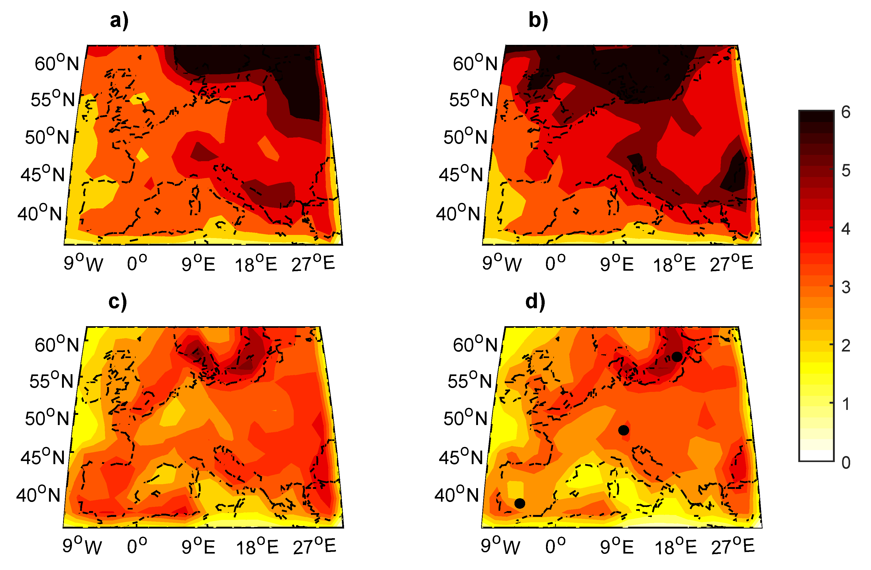
Figure 8.
Recurrences analysis for eight EURO-CORDEX runs at m = 1 years. Average biases of models (a) for hot temperature extremes EMM for (as in Figure 6c for CMIP5) and (b) for cold temperature extremes EMM for (as in Figure 6a for CMIP5). Standard deviation of the biases of models (c) for hot temperature extremes SDM for (as in Figure 7c for CMIP5) and (d) for cold temperature extremes SDM for (as in Figure 7a for CMIP5).


Table 1.
List of CMIP5 Models Analysed. The order is decreasing in resolution.
| No. | Model | Institution/ID | Country | Resolution |
|---|---|---|---|---|
| 1 | CMCC-CM | Centro Euro-Mediterraneo sui Cambiamenti Climatici | Italy | 0.75 × 0.75 |
| 2 | CCSM4 | National Center for Atmospheric Research, NCAR | USA | 1.25 × 0.94 |
| 3 | CESM1-BGC | Community Earth System Model Contributors, NCAR | USA | 1.25 × 0.94 |
| 4 | CESM1-FASTCHEM | Community Earth System Model Contributors, NCAR | USA | 1.25 × 0.94 |
| 5 | EC-EARTH | Danish Meteorological Institute, DMI | Denmark | 1.125 × 1.125 |
| 6 | MRI-CGCM3 | Meteorological Research Institute, MRI | Japan | 1.125 × 1.125 |
| 7 | BCC-CSM1-M | Beijing Climate Center | China | 1.125 × 1.125 |
| 8 | MRI-ESM1 | Meteorological Research Institute, MRI | Japan | 1.125 × 1.125 |
| 9 | CNRM-CM5 | CNRM-CERFACS | France | 1.40 × 1.40 |
| 10 | MIROC5 | MIROC | Japan | 1.40 × 1.40 |
| 11 | ACCESS 1-0 | CSIRO-BOM | Australia | 1.87 × 1.25 |
| 12 | ACCESS1-3 | CSIRO-BOM | Australia | 1.87 × 1.25 |
| 13 | HadGEM2-CC | MetOffice-Hadley Centre | UK | 1.87 × 1.25 |
| 14 | HadGEM2-ES | MetOffice-Hadley Centre | UK | 1.87 × 1.25 |
| 15 | HadGEM2-AO | MetOffice-Hadley Centre | UK | 1.87 × 1.25 |
| 16 | INM-CM4 | Institute for Numerical Mathematics, INM | Russia | 2 × 1.5 |
| 17 | IPSL-CM5A-MR | Institute Pierre Simon Laplace, IPSL | France | 2.5 × 1.26 |
| 18 | MPI-ESM-MR | Max Planck Institute for Meteorology, MPI | Germany | 1.87 × 1.87 |
| 19 | CMCC-CMS | Centro Euro-Mediterraneo sui Cambiamenti Climatici | Italy | 1.87 × 1.87 |
| 20 | CSIRO-MK3-6-0 | CSIRO-BOM | Australia | 1.87 × 1.87 |
| 21 | MPI-ESM-LR | Max Planck Institute for Meteorology, MPI | Germany | 1.87 × 1.87 |
| 22 | MPI-ESM-P | Max Planck Institute for Meteorology, MPI | Germany | 1.87 × 1.87 |
| 23 | FGOALS-2 | Institute of Atmospheric Physics, Chinese Academy of Sciences | China | 2.81 × 2.81 |
| 24 | NorESM1-M | Norwegian Climate Center | Norway | 2.5 × 1.89 |
| 25 | GFDL-ESM2G | Geophysical Fluid Dynamics Laboratory, NOAA | USA | 2.5 × 2.02 |
| 26 | GFDL-CM3 | Geophysical Fluid Dynamics Laboratory, NOAA | USA | 2.5 × 2.02 |
| 27 | GFDL-ESM2M | Geophysical Fluid Dynamics Laboratory, NOAA | USA | 2.5 × 2.02 |
| 28 | IPSL-CM5B-LR | Institute Pierre Simon Laplace, IPSL | France | 3.75 × 1.89 |
| 29 | BCC-CSM1-1 | Beijing Climate Center | China | 2.81 × 2.79 |
| 30 | MIROC-ESM | MIROC | Japan | 2.81 × 2.79 |
| 31 | MIROC-ESM-CHEM | MIROC | Japan | 2.81 × 2.79 |
| 32 | CMCC-CESM | Centro Euro-Mediterraneo sui Cambiamenti Climatici | Italy | 3.75 × 3.75 |
Order by horizontal resolution (Decreasing); Longitude × Latitude (); Centre National de Recherches Meteorologiques - Centre Européen de Recherche et de Formation Avancée en Calcul Scientifique; Atmosphere and Ocean Research Institute (University of Tokyo), National Institute for Environmental Studies, and Japan Agency for Marine-Earth Science and Technology; Commonwealth Scientific and Industrial Research Organisation(CSIRO), Bureau of Meteorology(BOM).
Table 2.
List of EURO-CORDEX bias corrected with EOBS10 used in this work. The experiment used was the control historical simulation (r1i1p1 ensemble member at of resolution).
Table 2.
List of EURO-CORDEX bias corrected with EOBS10 used in this work. The experiment used was the control historical simulation (r1i1p1 ensemble member at of resolution).
| No. | Model/Institution | Global | Regional | RCP Scenario |
|---|---|---|---|---|
| 1 | CNRM -CERFACS | CNRM-CM5 | CCLM4 | 45 |
| 2 | CNRM -CERFACS | CNRM-CM5 | CCLM4 | 85 |
| 3 | ICHEC -KNMI | EC-EARTH | RACMO22E | 45 |
| 4 | ICHEC -KNMI | EC-EARTH | RACMO22E | 85 |
| 5 | IPSL -INERIS | IPSL-CM5A-MR | WRF331F | 45 |
| 6 | IPSL -INERIS | IPSL-CM5A-MR | WRF331F | 85 |
| 7 | MPI -CSC | ESM-LR-MPI | REMO2009 | 45 |
| 8 | MPI -CSC | ESM-LR-MPI | REMO2009 | 85 |
Centre National de Recherches Meteorologiques; Centre Europeen de Recherche et de Formation Avancée en Calcul Scientifique (France); Ireland’s High-Performance Computing Centre (Ireland); The Royal Netherlands Meteorological Institute (Netherlands); Institut Pierre Simon Laplace (France); Institut national de l’environnement industriel et des risques (France); Max Planck Institute for Meteorology (Netherlands); Climate Service Center (Germany).
Table 3.
Statistical information extracted from the box plots of the biases (Figure 3) in hot and cold temperature extremes between models and 20CRv2c in 1900–1999 for two different bin lengths: m = 1 year and m = 4 years.
Table 3.
Statistical information extracted from the box plots of the biases (Figure 3) in hot and cold temperature extremes between models and 20CRv2c in 1900–1999 for two different bin lengths: m = 1 year and m = 4 years.
| No. | Model | Stand. Dev. | Mean | Skewness | % Outliers | Bin Length (m) | ||||
|---|---|---|---|---|---|---|---|---|---|---|
| min | max | min | max | min | max | min | max | |||
| 1 | CMCC-CMS | 1.97 | 0.99 | −6.89 | −2.56 | 0.43 | 0.02 | 22 | 16 | 1y |
| 1.82 | 0.90 | −3.42 | −3.51 | −0.18 | −0.14 | 24 | 35 | 4y | ||
| 2 | CCSM4 | 1.47 | 0.70 | 0.28 | 0.54 | 0.83 | −0.52 | 18 | 9 | 1y |
| 1.86 | 0.54 | 1.96 | 0.33 | 0.24 | −0.47 | 19 | 14 | 4y | ||
| 3 | CESM1-BGC | 1.31 | 0.71 | 1.33 | 0.57 | 0.53 | 1.04 | 19 | 15 | 1y |
| 1.14 | 0.69 | 0.73 | 0.08 | 0.45 | −0.43 | 9 | 9 | 4y | ||
| 4 | CESM1-FASTCHEM | 1.55 | 0.66 | 1.03 | 0.96 | 0.77 | 0.19 | 32 | 10 | 1y |
| 1.33 | 0.50 | 0.47 | 0.47 | 0.59 | −0.06 | 8 | 17 | 4y | ||
| 5 | EC-EARTH | 1.55 | 0.77 | 0.21 | −3.43 | 0.01 | −1.24 | 22 | 6 | 1y |
| 1.32 | 0.63 | 0.32 | −3.02 | −0.22 | −0.81 | 14 | 5 | 4y | ||
| 6 | MRI-CGCM3 | 1.16 | 0.90 | −2.28 | −1.43 | 1.37 | 0.20 | 12 | 7 | 1y |
| 1.85 | 0.45 | −2.42 | −2.08 | −0.20 | 1.19 | 16 | 6 | 4y | ||
| 7 | BCC-CSM1-M | 2.74 | 1.20 | 0.51 | −1.71 | 0.26 | −1.13 | 16 | 3 | 1y |
| 2.69 | 1.06 | 1.58 | −0.21 | 0.18 | 1.17 | 4 | 1 | 4y | ||
| 8 | MRI-ESM1 | 1.10 | 0.84 | −2.35 | −1.34 | 1.47 | 0.25 | 16 | 5 | 1y |
| 1.93 | 0.49 | −2.44 | −1.75 | 0.19 | 0.24 | 18 | 9 | 4y | ||
| 9 | CNRM-CM5 | 1.56 | 0.83 | −2.23 | 0.77 | −0.01 | 0.52 | 20 | 7 | 1y |
| 1.25 | 0.62 | −1.23 | 0.88 | 0.00 | −0.51 | 19 | 7 | 4y | ||
| 10 | MIROC5 | 1.43 | 0.64 | −0.04 | 2.00 | 0.23 | 0.80 | 21 | 2 | 1y |
| 1.26 | 0.49 | 3.13 | 1.62 | 0.35 | −0.08 | 20 | 2 | 4y | ||
| 11 | ACCESS 1-0 | 1.41 | 0.78 | 3.06 | −1.75 | 0.70 | 0.46 | 2 | 3 | 1y |
| 1.82 | 0.83 | 3.44 | −0.14 | −0.52 | −0.82 | 1 | 1 | 4y | ||
| 12 | ACCESS1-3 | 1.28 | 1.00 | 3.92 | 0.21 | 1.15 | 0.99 | 10 | 3 | 1y |
| 1.56 | 1.00 | 6.90 | 1.14 | −0.67 | −0.81 | 12 | 1 | 4y | ||
| 13 | HadGEM2-CC | 1.37 | 0.84 | −3.70 | −0.26 | 0.23 | 0.94 | 5 | 8 | 1y |
| 1.49 | 0.67 | −3.73 | −0.51 | −0.24 | 0.85 | 16 | 18 | 4y | ||
| 14 | HadGEM2-ES | 1.44 | 0.75 | −1.44 | 0.11 | 1.35 | −0.17 | 22 | 3 | 1y |
| 1.14 | 0.70 | −1.13 | 0.40 | −1.04 | 1.22 | 27 | 5 | 4y | ||
| 15 | HadGEM2-AO | 1.22 | 0.85 | −0.57 | 0.12 | 1.04 | 0.14 | 12 | 8 | 1y |
| 1.10 | 0.72 | −0.59 | 0.39 | −0.14 | 0.70 | 13 | 5 | 4y | ||
| 16 | INM-CM4 | 2.04 | 1.27 | −3.19 | 2.46 | 1.10 | −0.28 | 19 | 4 | 1y |
| 1.83 | 1.12 | −3.79 | 2.06 | 0.63 | −0.34 | 14 | 2 | 4y | ||
| 17 | IPSL-CM5A-MR | 1.86 | 0.86 | −0.86 | −0.76 | 0.49 | 0.66 | 34 | 10 | 1y |
| 1.95 | 0.64 | −1.09 | −0.83 | −0.09 | 0.15 | 23 | 5 | 4y | ||
| 18 | MPI-ESM-MR | 1.63 | 0.83 | −1.60 | −1.97 | −0.03 | 0.52 | 25 | 10 | 1y |
| 1.14 | 0.61 | 0.58 | −1.65 | −0.52 | 0.27 | 16 | 6 | 4y | ||
| 19 | CMCC-CMS | 1.89 | 1.00 | −4.88 | −2.29 | −0.02 | 0.02 | 21 | 23 | 1y |
| 1.89 | 0.87 | −2.12 | −3.04 | −0.40 | 0.05 | 42 | 19 | 4y | ||
| 20 | CSIRO-MK3-6-0 | 4.45 | 1.09 | −5.85 | −0.37 | 0.82 | 0.20 | 42 | 8 | 1y |
| 3.53 | 1.20 | −2.54 | −0.45 | −0.03 | −0.67 | 33 | 12 | 4y | ||
| 21 | MPI-ESM-LR | 1.65 | 0.66 | −0.92 | −2.63 | 0.40 | 0.16 | 31 | 2 | 1y |
| 1.29 | 0.62 | 0.74 | −2.05 | −0.49 | 0.46 | 13 | 6 | 4y | ||
| 22 | MPI-ESM-P | 1.38 | 0.74 | −0.42 | −2.01 | 0.55 | −0.22 | 34 | 17 | 1y |
| 1.45 | 0.50 | 1.28 | −1.87 | 0.20 | 0.55 | 16 | 10 | 4y | ||
| 23 | FGOALS-2 | 2.35 | 1.02 | 0.44 | 6.20 | 0.39 | −0.67 | 35 | 7 | 1y |
| 2.63 | 0.82 | −2.81 | 5.54 | 0.42 | −0.10 | 24 | 4 | 4y | ||
| 24 | NorESM1-M | 1.31 | 0.72 | 1.03 | −1.44 | 0.52 | −0.88 | 29 | 9 | 1y |
| 1.35 | 0.43 | 0.24 | −1.30 | 0.31 | −0.16 | 18 | 2 | 4y | ||
| 25 | GFDL-ESM2G | 1.53 | 0.86 | −3.42 | −0.81 | 0.20 | −0.24 | 14 | 8 | 1y |
| 1.35 | 0.56 | −2.74 | 0.11 | −0.07 | 0.65 | 6 | 12 | 4y | ||
| 26 | GFDL-CM3 | 1.51 | 0.94 | −1.88 | −2.20 | 0.14 | −0.84 | 14 | 4 | 1y |
| 1.61 | 0.63 | 1.47 | −0.69 | 0.05 | −0.37 | 2 | 24 | 4y | ||
| 27 | GFDL-ESM2M | 1.47 | 0.82 | −2.50 | −1.72 | 0.69 | −0.03 | 8 | 2 | 1y |
| 1.32 | 0.64 | −0.74 | 0.45 | −0.95 | −0.32 | 4 | 10 | 4y | ||
| 28 | IPSL-CM5B-LR | 1.90 | 1.05 | −9.51 | −0.57 | 0.05 | −0.72 | 26 | 20 | 1y |
| 3.28 | 0.81 | −10.06 | −1.74 | −1.83 | −1.58 | 29 | 5 | 4y | ||
| 29 | BCC-CSM1-1 | 1.98 | 0.68 | 0.16 | −2.37 | 1.84 | −0.37 | 7 | 2 | 1y |
| 2.42 | 0.89 | 0.58 | −0.84 | 0.34 | 0.54 | 9 | 1 | 4y | ||
| 30 | MIROC-ESM | 1.87 | 0.77 | 2.46 | −0.32 | −0.11 | −0.42 | 16 | 16 | 1y |
| 1.76 | 0.67 | 5.83 | 0.08 | −0.24 | −0.05 | 6 | 1 | 4y | ||
| 31 | MIROC-ESM-CHEM | 1.51 | 0.80 | 2.20 | −0.19 | −0.23 | −0.07 | 14 | 9 | 1y |
| 1.69 | 0.80 | 5.78 | 0.28 | −0.32 | −0.25 | 4 | 3 | 4y | ||
| 32 | CMCC-CESM | 1.74 | 0.79 | −4.65 | −2.18 | −0.23 | −0.42 | 13 | 4 | 1y |
| 2.23 | 1.02 | −7.01 | −3.26 | −0.04 | −0.32 | 10 | 22 | 4y | ||
| ENSEMBLE | 4.50 | 3.19 | −1.29 | −0.61 | 0.53 | −0.03 | 19 | 8 | 1y | |
| 5.01 | 2.98 | −0.39 | −0.46 | −0.13 | −0.01 | 15 | 9 | 4y | ||
© 2019 by the authors. Licensee MDPI, Basel, Switzerland. This article is an open access article distributed under the terms and conditions of the Creative Commons Attribution (CC BY) license (http://creativecommons.org/licenses/by/4.0/).
Share and Cite
MDPI and ACS Style
Alvarez-Castro, M.C.; Faranda, D.; Noël, T.; Yiou, P. Recurrence Spectra of European Temperature in Historical Climate Simulations. Atmosphere 2019, 10, 166. https://doi.org/10.3390/atmos10040166
AMA Style
Alvarez-Castro MC, Faranda D, Noël T, Yiou P. Recurrence Spectra of European Temperature in Historical Climate Simulations. Atmosphere. 2019; 10(4):166. https://doi.org/10.3390/atmos10040166
Chicago/Turabian StyleAlvarez-Castro, M. Carmen, Davide Faranda, Thomas Noël, and Pascal Yiou. 2019. "Recurrence Spectra of European Temperature in Historical Climate Simulations" Atmosphere 10, no. 4: 166. https://doi.org/10.3390/atmos10040166
Note that from the first issue of 2016, this journal uses article numbers instead of page numbers. See further details here.