Understanding Spatial Variability of Air Quality in Sydney: Part 1—A Suburban Balcony Case Study

Abstract

There is increasing awareness in Australia of the health impacts of poor air quality. A common public concern raised at a number of “roadshow” events as part of the federally funded Clean Air and Urban Landscapes Hub (CAUL) project was whether or not the air quality monitoring network around Sydney was sampling air representative of typical suburban settings. In order to investigate this concern, ambient air quality measurements were made on the roof of a two-storey building in the Sydney suburb of Auburn, to simulate a typical suburban balcony site. Measurements were also taken at a busy roadside and these are discussed in a companion paper (Part 2). Measurements made at the balcony site were compared to data from three proximate regulatory air quality monitoring stations: Chullora, Liverpool and Prospect. During the 16-month measurement campaign, observations of carbon monoxide, oxides of nitrogen, ozone and particulate matter less than 2.5-µm diameter at the simulated urban balcony site were comparable to those at the closest permanent air quality stations. Despite the Auburn site experiencing 10% higher average carbon monoxide amounts than any of the permanent air quality monitoring sites, the oxides of nitrogen were within the range of the permanent sites and the pollutants of greatest concern within Sydney (PM_2.5 and ozone) were both lowest at Auburn. Similar diurnal and seasonal cycles were observed between all sites, suggesting common pollutant sources and mechanisms. Therefore, it is concluded that the existing air quality network provides a good representation of typical pollution levels at the Auburn “balcony” site.

1. Introduction

Air quality in Sydney is relatively good compared to other large industrialised cities [1]. Background ozone concentrations in Sydney are comparatively low: the annual mean ozone concentration for Sydney was 18.5 ppb in 2017 [2]. In comparison, the 2017 mean ozone concentration for urban sites in the UK was 27.9 ppb [3]. In New South Wales (NSW), measured particulate matter (<2.5 μm diameter; PM_2.5) concentrations are generally <15 µgm⁻³, but occasionally exceed the national daily standard (25 µgm⁻³) particularly during wildfire events [4]. Despite the relatively low levels of harmful air pollutants measured in Sydney, air quality constitutes a health risk in the city. It has been established that exposure to some pollutants, including ozone and PM_2.5, at concentrations considered generally safe by the US EPA is nevertheless associated with negative health outcomes [5,6]. Furthermore, approximately 2% of deaths in Sydney have been attributed to ozone and particulate pollution [1]. These species dominate exceedances of national air quality standards in Sydney [2,7]. Ozone and particulate matter have therefore been identified as pollutants of most concern in Sydney. Ozone exceedances in Sydney are associated with very high summer temperatures, with influence from both synoptic [8] and mesoscale [9] meteorological variables. The Sydney region predominantly experiences a NO_x-limited regime during ozone events, with the influence of biogenic emissions highlighted in recent literature [10]. Despite the strong influence of bushfires and dust storms on PM_2.5 exceedances [11,12], traffic emissions have been shown to be the largest single source of PM_2.5 within the Sydney basin [13].

Methods used to gather ambient air quality data largely utilise fixed-site ground-level monitoring stations often located in local parks that measure background pollutant concentrations. For example, the New South Wales Office of Environment and Heritage (OEH) maintains a network of permanent, stationary air quality monitoring stations throughout Sydney [2].

Increasing population in Sydney is driving increased construction of (and residence in) apartment buildings. Apartment buildings accounted for one-third of all new residential building approvals in Australia in 2015, with more than 30% of these in Sydney [14]. As of the 2016 census, 20.7% of residences in New South Wales were apartments, with greater than 85% of these apartments located in Sydney [15]. Therefore, it is reasonable to assume that urban balconies are a site of possible exposure to poor air quality for a significant proportion of the population of Sydney.

A small body of research exists discussing the effect of balconies on ventilation impacting indoor air quality in high rise buildings [16,17] and regarding pollutant mixing in urban street canyons [18]. However, limited research exists regarding air quality measurements at balcony sites. Nevertheless, general research into vertical changes in urban air quality has been more thoroughly researched. Ozone has been modelled to vary with height above street level. The presence of other ozone-destroying compounds in urban areas is modelled to deplete surface ozone up to altitudes of 20 m [19]. This phenomenon has been measured in Beijing [20], with the effect of shears in wind speed and wind direction highlighted. Several studies have found that PM_2.5 concentrations decrease with increased height in an urban environment [21,22]. Contrastingly, a study on multi-storey buildings in Singapore showed that mean PM_2.5 concentration was highest at the mid-floors in comparison to upper and lower floors, and the upper floors had the lowest fine particular matter mass concentration [23]. It was noted, however, that this may have been the result of particle interception by surrounding tree leaves and inflow of cleaner air from higher altitudes. Han et al. [24] found that measurement sites at near-ground height (5–10 m) were most influenced by human emission activities compared to measurements at higher altitudes. It has been noted that a number of factors influence the vertical profiles of PM_2.5 concentrations, including vehicle emissions and new particle formation [25]. Urban street canyons and the presence of neighbouring buildings have also been shown to play a role by altering vertical mixing and flow fields [18].

The Clean Air and Urban Landscapes (CAUL) hub is a project of the National Environmental Science Program, which is funded by Australia’s Department of the Environment and Energy. CAUL focuses on cross-disciplinary research on the sustainability and liveability of Australian urban environments [26]. Air quality is an important part of this investigation. CAUL research is partially driven by public concerns expressed at a number of “roadshow” events. A recurring question posed by members of the public was “how does the background air quality reported for my area relate to my likely exposure when I am outside?” Although we acknowledged that we cannot answer this question for any particular individual, we nevertheless set about trying to address this problem via the use of two separate case studies:

• WASPSS-Auburn (Western Air-Shed Particulate Study for Sydney in Auburn)—provides an assessment of whether the local air quality monitoring stations give a good representation of pollutant concentrations at a site representative of a suburban balcony setting.
• The RAPS campaign (Roadside Atmospheric Particulates in Sydney) provides an assessment of PM_2.5 concentrations near a busy road in the Sydney City metropolitan area, and how these compare to reported air quality levels from nearby statutory monitoring stations. The spatial and temporal variability of PM_2.5, relevant to members of the public seeking to minimise their exposure to fine particulate matter, are also explored. The campaign also provided an opportunity for the first calibration of a microscopic traffic emissions simulation.

The first case study is discussed in the present paper, and the second is covered in a companion paper, also in this issue [27].

The WASPSS-Auburn campaign incorporated a mobile air quality monitoring station and an open-path infrared Fourier transform spectrometer (OP-FTIR). The OP-FTIR system, which can measure infrared active gases such as CO, NH₃, N₂O and CH₄, has previously been deployed for agricultural [28,29,30] and biomass burning [31,32] emissions estimates. Details of the main findings from the OP-FTIR during WASPSS, which relate to vehicle ammonia emissions and episodes of significant smoke pollution, are presented in two separate papers [33,34].

In this paper we present the results from the mobile air quality monitoring station during the 16-month WASPSS-Auburn campaign at the simulated suburban balcony site and compare the pollution levels observed to those measured at the closest permanent air quality monitoring stations. Local-scale phenomena, including the built environment and meteorological processes, dominate vertical variability in urban pollutant concentrations, especially particulates and ozone, making it very difficult to generalise findings at any one site to a broader region; however this is not the purpose of this study. Instead, we aim to observe the similarities and differences between pollutant concentrations at a simulated urban balcony site and regional air quality monitoring stations and test the assumption that regional background measurements provide a reasonable representation of pollutant concentrations to which local residents may be exposed to on an urban balcony.

2. Methodology

2.1. The Mobile Air Quality Station

The Mobile Air Quality station (MAQ) (inset, Figure 1) is a mobile compact air quality station that complies with the Australian/New Zealand Standards for the measurement of ambient air quality, National Environmental Protection (Ambient Air Quality) Measure (NEPM) [35]. The MAQ is fitted with the following instruments.

• Model T204 Teledyne NO_x + O₃ Analyser
• Model T300 Teledyne CO Analyser
• Model 100E Teledyne SO₂ Analyser
• Thermo Scientific TEOM Series Model 1405-DF (used for reported PM_2.5 and PM₁₀ measurements)
• Ecotech Aurora 3000 multi wavelength integrating Nephelometer
• Met-One 50.5 sonic wind sensor
• Vaisala HMP155 Temperature and Humidity Sensor

Calibration and communications equipment was also installed, allowing quality control and monitoring of the instrumentation. Measurements were taken at one-minute time resolution and averaged to one hour mean values. Maintenance and calibration were performed in accordance with Climate and Atmospheric Science Standard of Operation Procedures [36]. Note that all observations described in this paper are from the MAQ station unless explicitly stated otherwise. Further details on the measurements are publicly available [37].

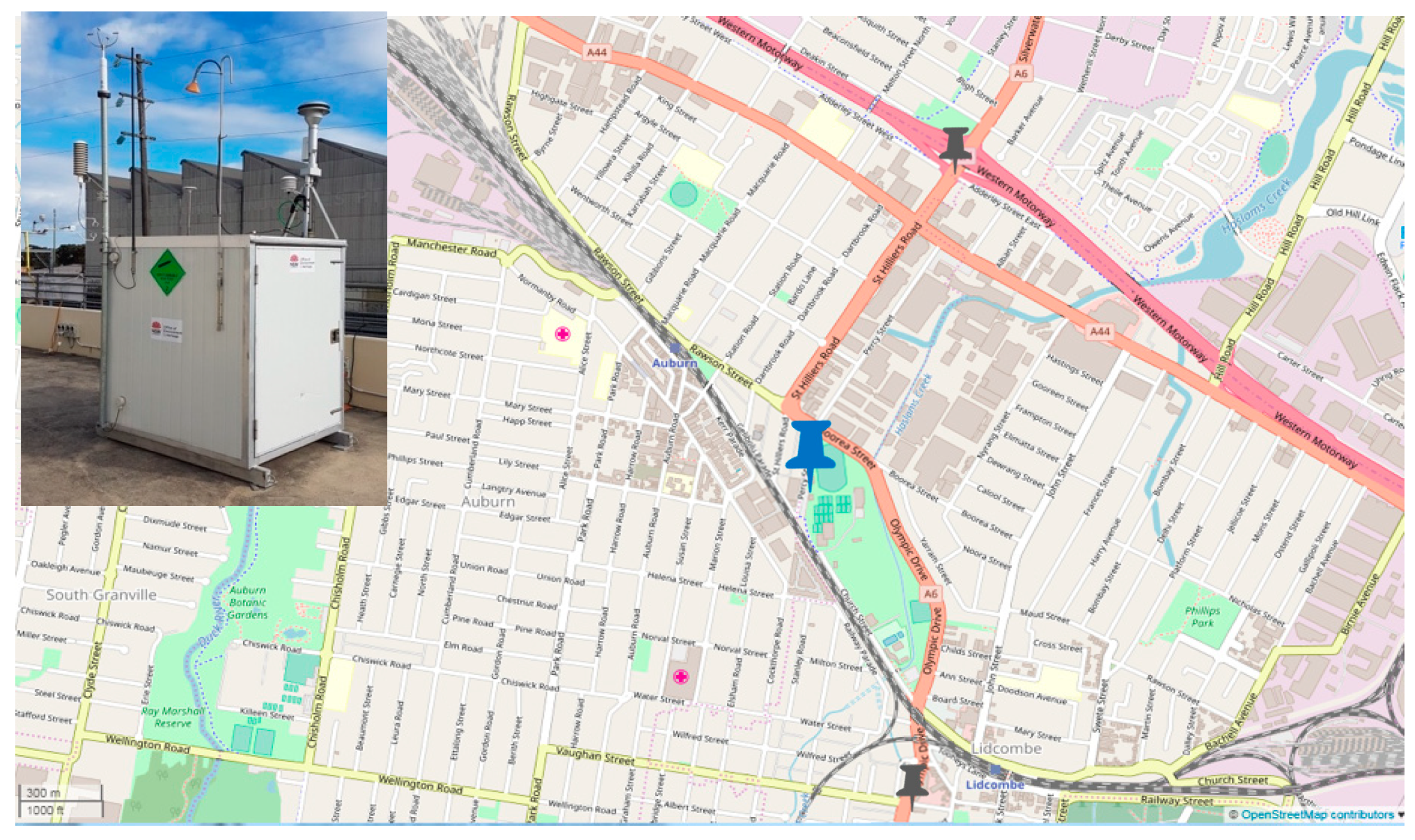
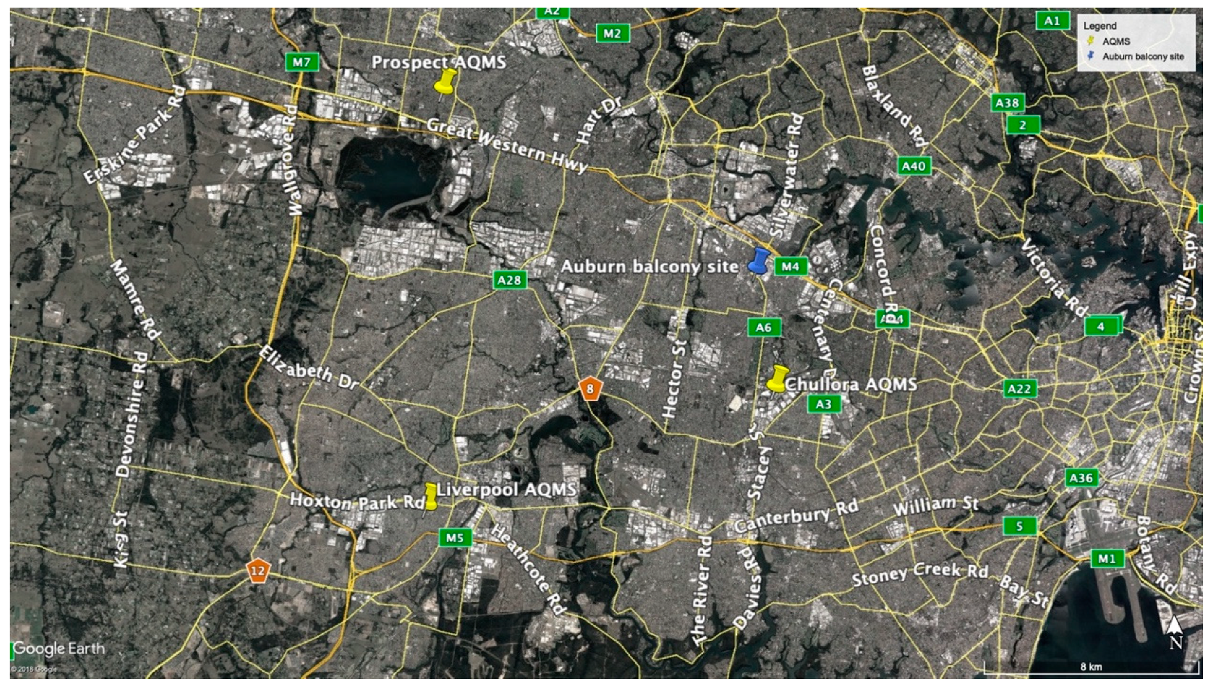
2.2. Auburn Balcony Measurement Site

Auburn is a suburb in Western Sydney that is located 16 km west of downtown Sydney (measured from Sydney Harbour Bridge) containing residential, business and industrial areas, as well as numerous parks and sporting complexes. On the 23 May 2016 the MAQ station was placed on site on the roof of the second storey of a commercial business at 2 Percy Street, Auburn, (33.854690° S, 151.037400° E, 6.72 m above ground level, 20.6 m above sea level). This site was chosen purely for pragmatic reasons, as we had connections to allow us access to the roof (and gained permission to locate the retroreflectors for the open-path measurements on the council building 400 m away across the town centre). However, Auburn is a good representative suburban centre with a good mixture of land uses including residential, industrial and transport. The MAQ inlet height was 3.3 m above the rooftop. The Auburn site (Figure 1 main image) is adjacent to a major rail passageway, with several industrial sites in the vicinity. There is a nearby major intra-urban road (A6) situated 330 m to the east of the site with the Great Western highway (A44) and the M4 motorway, also runs from north to east, at distances of just over 2 km from the site. Measurements are available from 26 May 2016 until 18 September 2017. Data from the MAQ and from the Open Path FTIR and associated instruments are available at the Pangaea Data Publisher [37].

2.3. Chullora, Prospect and Liverpool Air Quality Monitoring Stations

The OEH monitors air quality in urban areas of New South Wales using strategically placed air quality monitoring stations. These sites are equipped with instrumentation sufficient to meet the Ambient Air Quality NEPM [38], with measurements taken using a standard sampling protocol and undergoing rigorous quality assurance [39]. Instrumentation at permanent sites is different to that used in the MAQ station, with specifications for each site being publicly available [40]. This allows the OEH to provide current data online publicly and allows for comparison between network sites. Measurements taken at the Auburn balcony site were compared with the following three air quality monitoring stations in western Sydney: Chullora, Liverpool and Prospect.

• Chullora air quality monitoring station (33°53′38″ S, 151°02′43″ E, 32 m above sea level), is located in the grounds of the Southern Sydney TAFE, Worth St, Chullora, in a mixed residential and commercial area. Nearby traffic influences include the A6 and Hume Highway, both within 0.5 km from the site and with a major road joining the two approximately 150 m to the south.
• Liverpool air quality monitoring station (33°55′58″ S, 150°54′21″ E, 22 m above sea level) is located in the Council depot, off Rose Street, Liverpool, in a mixed residential and commercial area. The Hume Highway and M5 motorway are both within approximately 1 km of the site.
• Prospect air quality monitoring station (33°47′41″ S, 150°54′45″ E, 66 m above sea level) is located in William Lawson Park, Myrtle Street, Prospect, in a residential area. The Great Western Highway lies approximately 1 km to the south, with the M4 motorway a further 400 m south.

These sites were selected as they are the most proximate stations (within 15 km) to the Auburn site, located to the southwest, southeast and northwest, respectively (Figure 2). Each of these stations is located in or adjacent to reserves of parklands. Publicly available hourly measurements from each air quality monitoring station were downloaded from the OEH website [41].

2.4. Traffic Counters

Measurements from two traffic counters, located on Olympic Drive (station 7153, 1.25 km SSE of Auburn balcony) and on Silverwater Road (station 7112, 1.40 km NNE of Auburn balcony), were used to assist with pollutant analysis (see Figure 1 for locations). Traffic counters are maintained by the New South Wales Roads and Maritime Services. Hourly measurements of total vehicle count from 26 May 2016 to 13 September 2017 were downloaded for each site and processed to mean hourly counts during the measurement period. Both cameras count traffic travelling northbound on the A6. Data is publicly available from the Roads and Maritime Services website [42].

2.5. Data Analysis

Variables selected for analysis were wind speed, temperature, carbon monoxide (CO), oxides of nitrogen (NO_x), ozone (O₃) and PM_2.5. Meteorological variables were chosen to account for the effect of temperature and wind speed on pollutant concentrations. Ozone and PM_2.5 have been identified as pollutants of most concern in Sydney and were therefore critical to the project. CO and NO_x were analysed as they are associated with traffic emissions and interact with and influence concentrations of the pollutants of most concern.

Data were analysed using the software “R” (version 3.4.0) [43] making extensive use of the “openair” package (version 2.6.1) [44]. Mean statistics reported refer to the entire measurement campaign. Mean bias values were calculated using the openAir “modStats” package [44] and are expressed as a percentage of the overall mean value for the variable at the Auburn balcony site.

The percentage of valid data collected over the measurement period was as follows for the analysed variables; temperature and wind speed: 100%; CO: 94%; NO_x: 78%; O₃: 60.1%; PM_2.5 and PM₁₀; 99%.

3. Results and Discussion

Measurements from the Auburn balcony site were compared to the regional background concentrations as measured by three proximal air quality monitoring stations located at Chullora, Liverpool and Prospect.

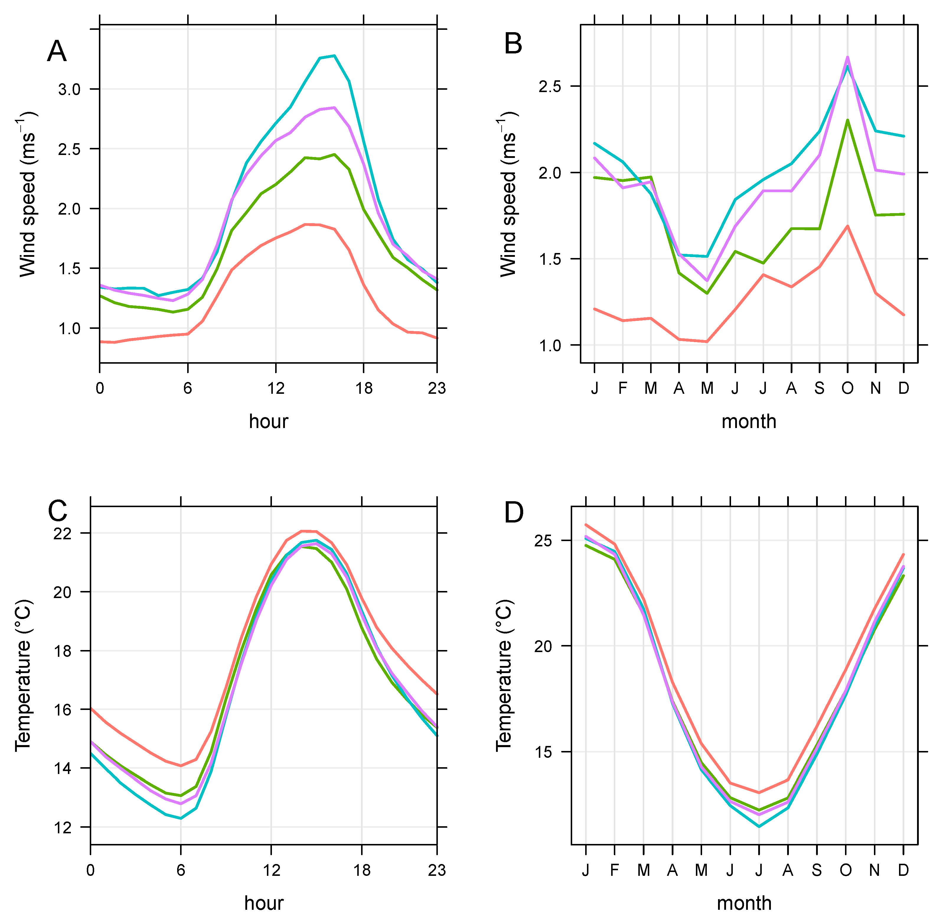
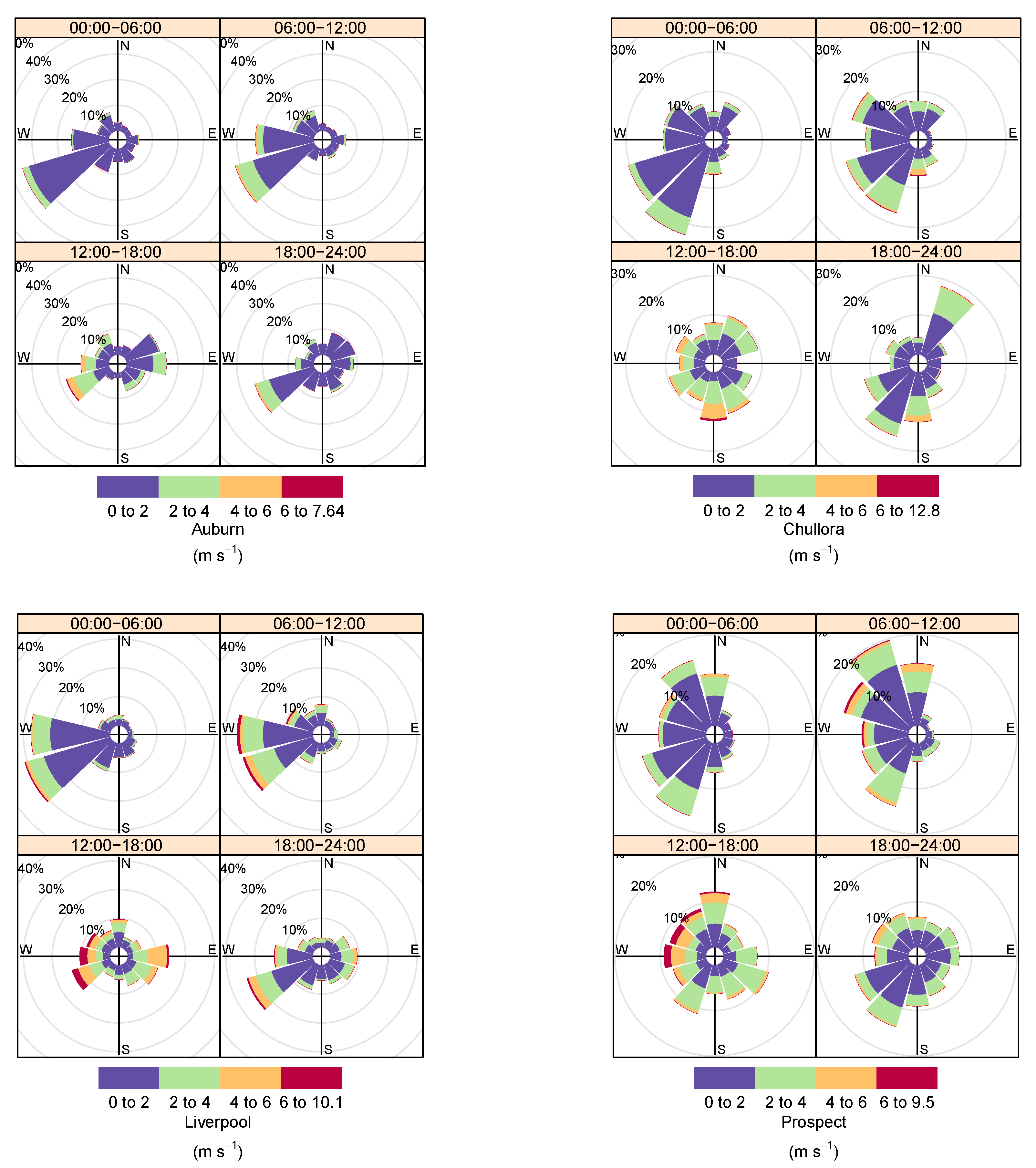
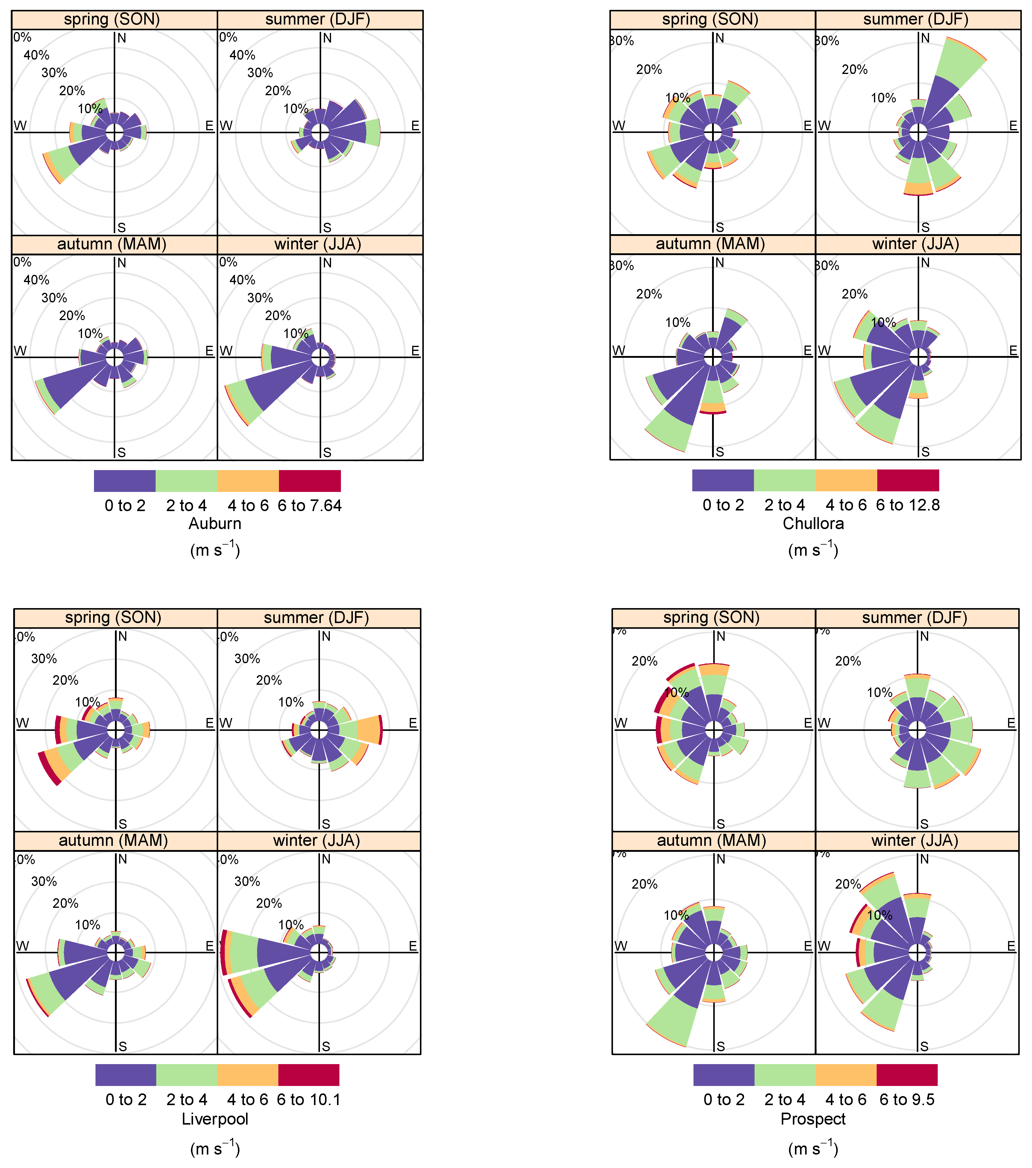
3.1. Wind and Temperature

Examination of wind speed measurements revealed that the Auburn balcony has a diurnal cycle similar to the background sites (Figure 3A). At each location, the wind speed is lowest overnight and into the morning (23:00–06:00). Wind speed then increases through the morning, peaking between 12:00 and 18:00, before dropping back to a minimum late in the evening. All permanent air quality monitoring sites display higher wind speeds throughout the 24-h cycle than the balcony site. This is reflected by a lower mean wind speed at Auburn (1.3 ms⁻¹) compared to Chullora, Liverpool and Prospect (1.7, 2.0 and 1.9 ms⁻¹, respectively). The average mean bias between Auburn and the air quality monitoring stations is −47%. This is likely to be due to the positioning close to buildings dampening the measured wind speed at Auburn, compared to the measurements in more open areas at the permanent air quality stations.

Plotting monthly mean wind speeds demonstrates that all sites follow the same annual trend (Figure 3B) containing an autumn minimum in May and an October spring maximum. The similarity in seasonal cycle between sites is unsurprising considering their relatively close proximity. Lower wind speeds at Auburn are again evident throughout the cycle.

Temporal variations in wind direction were also examined. Measurements were binned into four periods—00:00–06:00, 06:00–12:00, 12:00–18:00, and 18:00–00:00—for each site and plotted as wind roses (Appendix A, Figure A1). Winds until 12:00 at all sites were dominated by SW winds at all sites, with a northerly flow also evident at Prospect. Winds appeared more variable in the afternoon and evening with a greater variability in wind direction evident. Variability observed between sites is unsurprising given the sensitivity of local surface winds to the environment immediately surrounding the measurement site.

Seasonality is observed in wind direction at all sites. Site specific wind roses, binned by season, are presented in the Appendix A, Figure A2. Spring and summer winds are the most variable at all sites, with noted northerly airflows observed at Chullora, and easterly flows at Liverpool during summer. Southerly and westerly flows dominate winter winds at Auburn, Chullora and Liverpool, with a distinctive NW flow evident during winter at Prospect.

Analysis of mean hourly temperature (Figure 3C) again reveals a similar cycle at all sites, with minimum temperatures experienced just prior to sunrise, and building to a maximum in the early afternoon. Auburn is slightly warmer overnight and during early hours of the morning than other sites. The average mean temperature bias of the Auburn balcony compared with the air quality monitoring stations is close to 1 °C warmer, perhaps due to the thermal retention properties of the concrete Auburn rooftop as compared to the parkland sites of the other air quality monitoring stations.

A plot of mean monthly temperatures (Figure 3D) displays the expected seasonal cycle at all sites. Temperature is at its highest (close to 25 °C) during summer, with the winter minimum temperature experienced in July. Geographical proximity is again responsible for similarity in the seasonal temperature cycle. Again, slightly warmer temperatures are observed at Auburn compared to other sites. This is particularly noticeable in the cooler months.

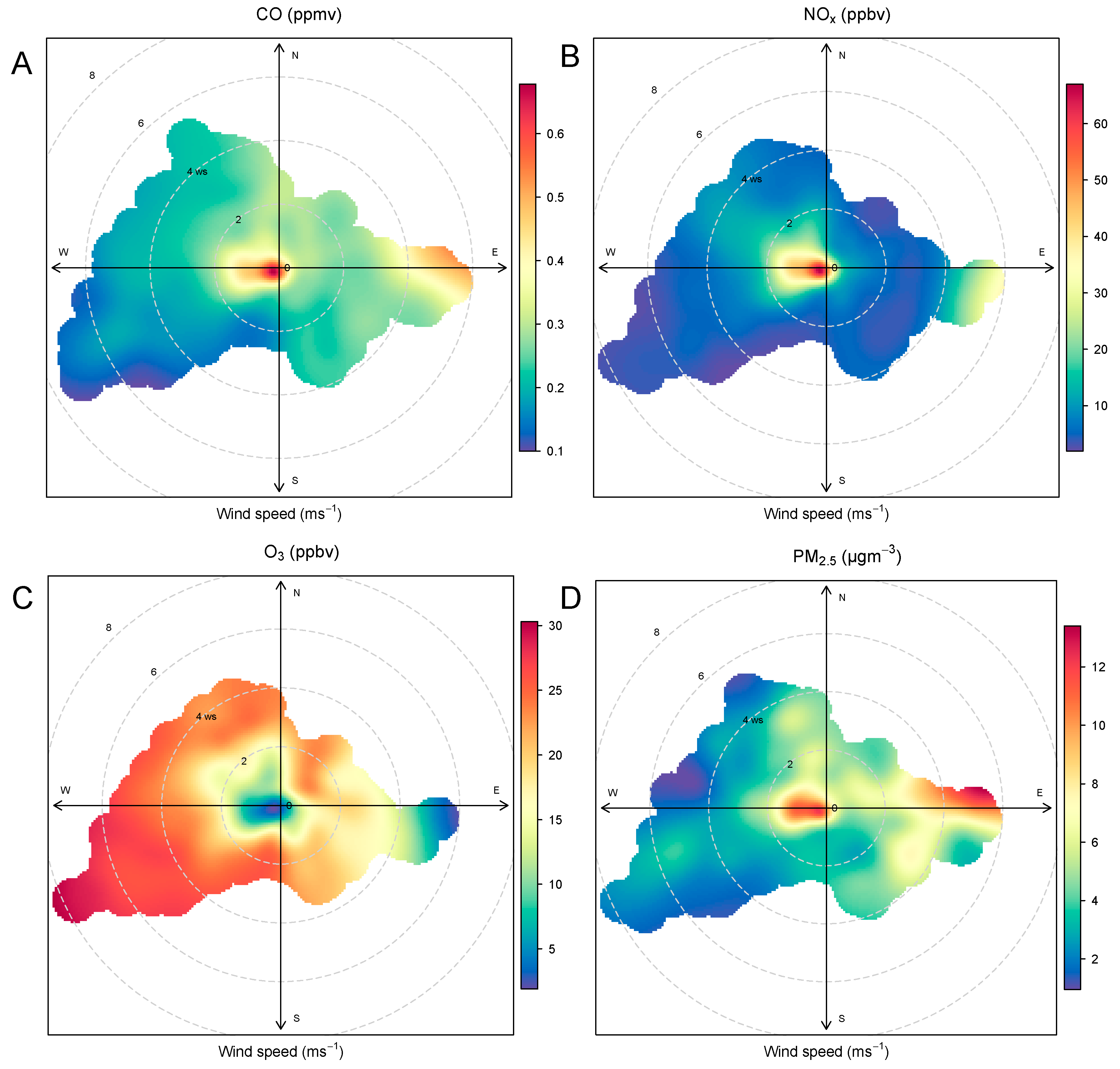
3.2. Carbon Monoxide, Oxides of Nitrogen and Ozone

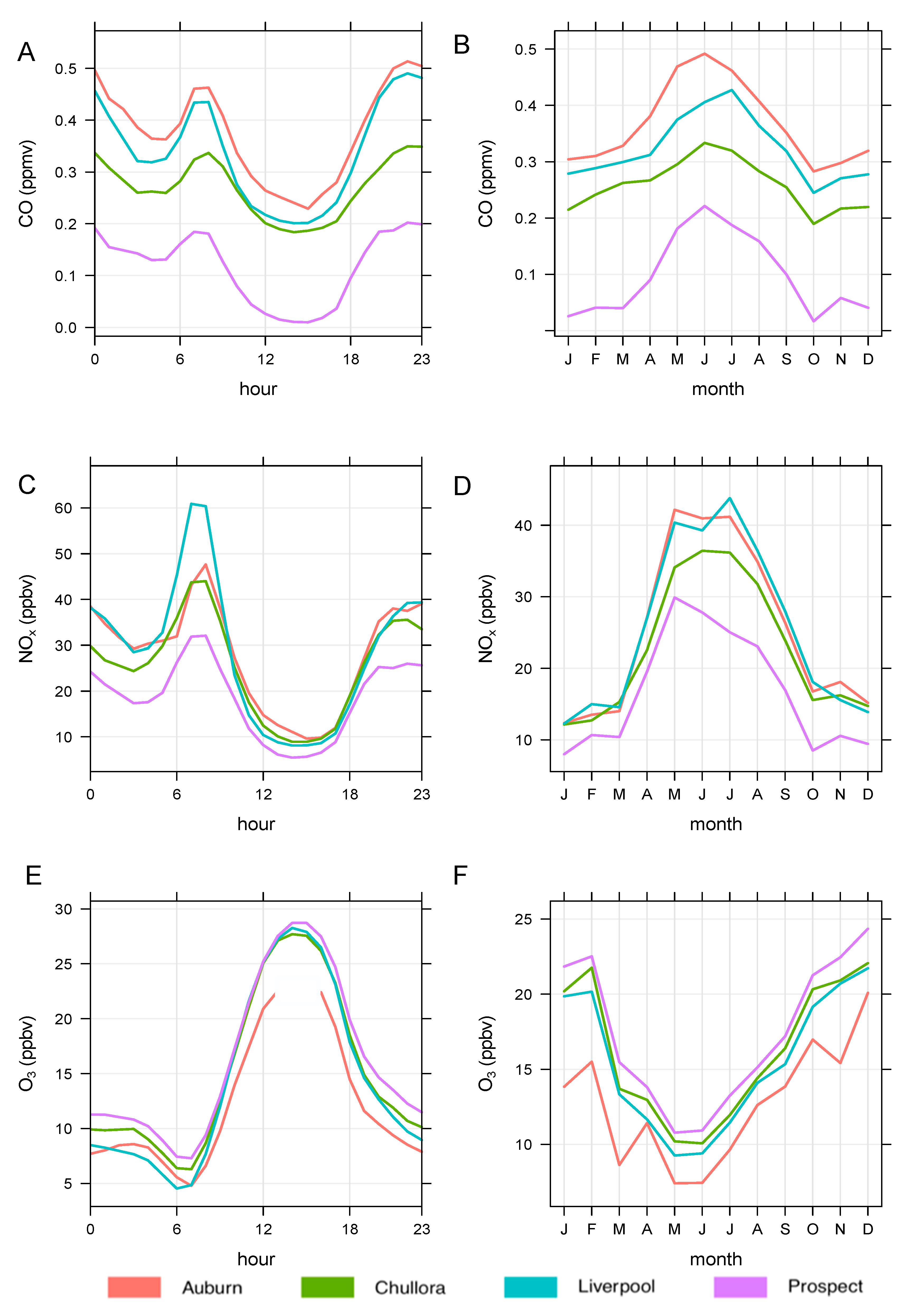
3.2.1. Carbon Monoxide

Diurnal and seasonal cycles of CO, NO_x and ozone are presented in Figure 4. A plot of hourly mean CO mole fraction (Figure 4A) displays a bimodal distribution at all sites. CO pollution begins growing at 05:00, reaching a first peak between 07:00 and 08:00. A decrease from this peak gives diurnal minimum concentrations in the early afternoon, coincident with the timing of peak wind speeds (Figure 3A). The evening peak grows from near 17:00 to a maximum near 22:00. The mean CO mole fraction measured at Auburn (0.38 ppm) is similar, albeit slightly higher than that measured at Chullora (0.27 ppm) and Liverpool (0.33 ppm). The mean CO mole fraction at Prospect is significantly lower (0.11 ppm), with lower amounts evident throughout the diurnal cycle. This is reflected in the mean bias between Auburn and the air quality monitoring stations as ranging from +10% (compared to Liverpool) to +68% (compared to Prospect). The significantly lower CO mole fractions at Prospect (which is in a residential area) suggest that the commercial activities near the other sites contribute a substantial fraction of the CO pollution at Auburn, Chullora and Liverpool (that are all mixed residential and commercial areas).

3.2.2. Oxides of Nitrogen

Plotting hourly mean mole fractions of oxides of nitrogen (NO_x, Figure 4C) reveals a similar bimodal distribution at all locations. The first peak occurs between 07:00 and 08:00, with the broader second peak occurring between 19:00 and 22:00. Morning maximum NO_x pollution varies between sites from an average of 60 ppb at Liverpool to an average of almost 30 ppb at Chullora. During the evening peak, NO_x pollution levels at the different sites are more similar to each other especially at Auburn, Liverpool and Chullora. The broadening observed in the evening peak is likely to be caused by a coupling of the evening traffic peak and the collapse of the daytime boundary layer. Again, hourly NO_x mole fractions are consistently lower at Prospect than at the other sites. This is reflected in a significantly greater mean bias between Auburn and Prospect (+32%) compared to Auburn and Chullora (+6.9%), and Auburn and Liverpool (−5.3%). Mid-afternoon minimum NO_x pollution is observed at all sites in a similar manner to minimum CO pollution.

3.2.3. Traffic as a Major Source of Carbon Monoxide and Oxides of Nitrogen

The similarity in diurnal cycles implies that a common source of CO and NO_x dominates at all measured locations. It is suggested that the diurnal cycle is related to morning and evening rush hours at all sites, with high overnight concentrations attributable to low boundary layer conditions [45,46]. Examining traffic counts along this road supports this attribution. Northbound traffic along the A6 (300 m east of the balcony site) shows a morning peak at 06:00–08:00 at sites both north and south of the Auburn balcony (Figure 5). This aligns with the morning peak in CO and NO_x. This suggestion is further supported by examining polar bivariate plots of the Auburn balcony site. The slightly elevated pollution levels of CO and NO_x associated with relatively strong easterly winds (Figure 6A,B) is likely attributable to the A6 highway. An explanation for mid-afternoon minimum pollution levels is found when examining diurnal wind speed patterns. Wind speed and CO/NO_x amounts are anticorrelated. During the mid-afternoon, turbulence and local wind speed are at maximum (Figure 3A). This leads to a deep boundary layer and hence more pollutant dilution.

High pollutant mole fractions at low wind speeds for CO and NO_x in Figure 6 indicate local pollutant sources, because during periods of very low wind speed pollutant transport is supressed. High pollution levels during low wind speeds also suggest accumulations in periods of atmospheric stability. In addition to local traffic and domestic emissions mentioned, there are industrial facilities proximate to the Auburn site contributing to the observed CO and NO_x levels, as documented in Australia’s National Pollutant Inventory. Five-hundred metres to the NE of the Auburn balcony is a printery, emitting 2.8 Tyr⁻¹ CO and 4.2 Tyr⁻¹ NO_x [47]. Nine-hundred metres to the NE is a major brewery, emitting 31 Tyr⁻¹ CO and 150 Tyr⁻¹ NO_x [48]. The higher pollution associated with wind speeds between 1 and 2 m s⁻¹ from the West is likely the result of katabatic drainage associated with highly stable conditions and low atmospheric mixing that traps urban pollution close to the ground-level [45,46].

3.2.4. Ozone

Typical diurnal cycles of ozone are observed when plotting hourly means across a 24-h period (Figure 4E) at the Auburn balcony sites, and at the Chullora, Liverpool and Prospect air quality monitoring stations. There is a pre-dawn minimum of less than 10 ppb at all sites growing to a mid-afternoon maximum greater than 20 ppb, due to the daytime photochemical production of ozone followed by titration of ozone by NO overnight. The relationship between NO_x and ozone is evident in the anticorrelation between the species (correlation coefficient, r = −0.57, number of points, n = 38,869). This is also evident when comparing the polar bivariate plot of NO_x (Figure 6B) to that of ozone (Figure 6C), and also in the diurnal cycles of the species (Figure 4C,E, respectively). The relationship between ozone and temperature is also clearly expressed in these measurements (r = 0.63, n = 39,539). Ozone levels are similar between sites, except during summer when ozone is significantly lower at the Auburn balcony site than at the proximate air quality monitoring stations. However, it must be noted that a reduced number of ozone measurements were taken during the summer maximum at the Auburn site. This may contribute to the lowered average concentration. Calibration of the ozone instrument occurred at 14:00 or 15:00 each day, creating a lack of measurements during the daily ozone peak. This also contributes to the lower concentrations (average mean bias: −24%) reported at the Auburn balcony compared to the other sites.

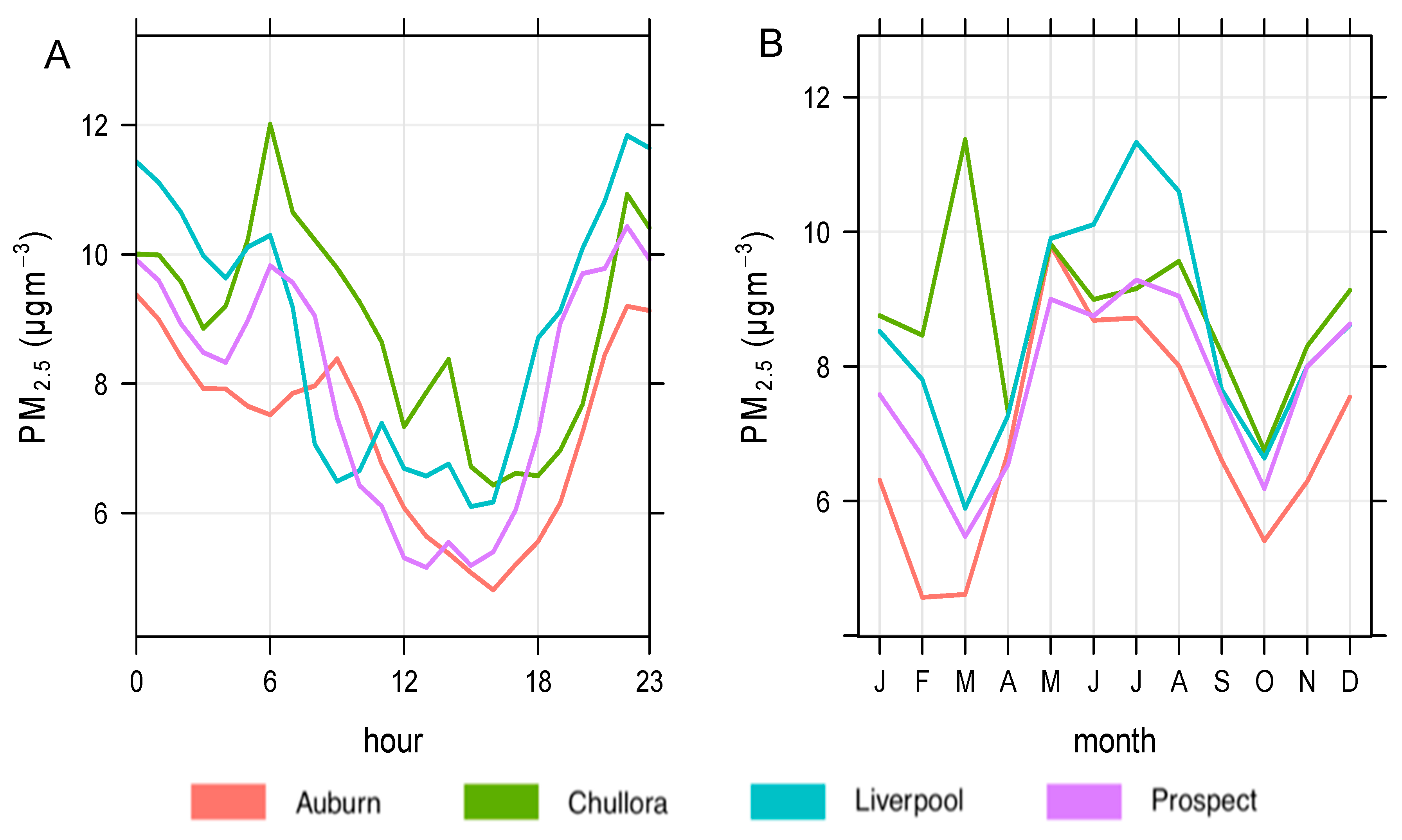
3.2.5. Annual Cycles of Carbon Monoxide, Oxides of Nitrogen and Ozone

Monthly means of CO and NO_x (Figure 4B,D, respectively) reveal similar seasonal cycles for these species. Highest pollution levels for both pollutants at all sites are observed in May, June or July. Higher winter mole fractions are attributed to a combination of factors: slower photochemical removal, lower boundary layer mixing heights and additional contributions to CO and NO_x from combustion heating. CO and NO_x are lower at Prospect than at other sites throughout the year. Again, a dependence on wind speed is evident, with the seasonal cycle of wind speed (Figure 3B) anticorrelated with those of CO and NO_x (Figure 4A,C).

Monthly mean ozone mole fractions (Figure 4F) also align with the expected seasonal cycle at all sites. A December maximum is observed at all sites, coinciding with the period of peak solar irradiance and high summer temperatures. This agrees with previous studies regarding ozone in the Sydney basin, with the importance of extreme heat and biogenic emissions noted [10,49,50]. The May–June minimum is aligned with less daylight hours and cooler temperatures, giving rise to slower photochemistry and less ozone production. Mean mole fractions throughout the year are similar for the three air quality monitoring stations. Ozone measurements are lower at Auburn throughout the year, with the greatest difference observed in late summer, partly due to the reasons previously stated.

3.3. PM_2.5

Plotting hourly mean PM_2.5 concentration (Figure 7A) reveals, as with other pollutants, a similar diurnal cycle between measurement locations. The four sites follow a similar bimodal trend, where the PM_2.5 concentration is at a maximum near 06:00, and again in the evening. The higher concentration of PM_2.5 during the evening and into the night is most likely the particulates being trapped within the low nocturnal boundary layer.

A likely source of particulate pollution at all sites is local traffic, similar to CO and NO_x. The trough present in early afternoon PM_2.5 concentration is likely due to the growth of a turbulent boundary layer. Evidence for particulate dilution is provided in maximum wind speed coincident with minimum particle concentrations in the mid-afternoon (Figure 3A), and minimums in the morning and evening during high observed concentrations of PM_2.5. Auburn shows mean concentrations comparable to the other sites, although the morning peak is later than at the other sites, suggesting a possible influence of local traffic that could be associated with school drop-off times. The mean bias for the Auburn balcony with each site is Chullora −1.29 µgm⁻³, Liverpool −1.42 µgm⁻³ and Prospect −0.640 µgm⁻³. Negative values in each instance show that the Auburn balcony sees slightly lower mean PM_2.5 than each permanent site. The polar bivariate plot for Auburn (Figure 6D) shows the impact of the nearby A6 motorway when winds are from the east. Secondary particulate formation is driven by regional scale processes within the Sydney basin, since the precursors are dominated by biogenic sources from the surrounding forested regions. For this reason, photochemically driven particle formation processes are not expected to contribute significantly to differences between PM_2.5 concentrations at the different sites.

Annual trends in PM_2.5, examinable by plotting monthly mean concentrations (Figure 7B), are also similar between all sites. The most notable exception is a very high March mean at Chullora, which is not present at other sites. This localised increase in monthly mean concentration is attributable to a fire that occurred on 22 February 2017 at a recycling plant less than one kilometre from the AQMS [51]. Reduced February and March concentrations at Auburn may be an artefact of a period of reduced measurements due to technical difficulties. All sites show a winter maximum, likely attributable to combustion heating emissions [33]. A smaller, secondary maximum in December–January is due to more active secondary photochemical particle formation processes (partially temperature and oxidant driven) [52]. The influence of wind speed on PM_2.5 is also clear when comparing the annual cycle of wind speed (Figure 3A) to that of PM_2.5 (Figure 7B), with the two annual cycles anticorrelated.

Diurnal and seasonal cycles of PM₁₀ were also plotted. The diurnal cycle (provided in the Appendix A, Figure A3A) is very similar to that of PM_2.5 at all sites. The seasonal cycle (Appendix A, Figure A3B) varies significantly, showing summer maxima at all sites and no winter peak. Similar to PM_2.5, PM₁₀ concentrations at Auburn are lower than those at all permanent sites as indicated by mean bias (Chullora: −2.26 µgm⁻³; Liverpool: −3.24 µgm⁻³; Prospect: −1.53 µgm⁻³).

4. Discussion—Comparison of Balcony Site to Regional Background

The Auburn balcony site demonstrates similar diurnal and seasonal cycles to nearby permanent air quality monitoring stations sites for all analysed variables. This implies that similar mechanisms are driving variability in pollutant concentrations observed at the balcony site and at regional background sites. There is some difference in pollution levels (amplitude of diurnal and seasonal cycles) between sites. Auburn recorded lower wind speed than those recorded at the air quality monitoring stations and slightly higher temperatures. Higher levels of carbon monoxide were observed at Auburn that at any of the other three sites.

Diurnal and seasonal cycles of the pollutants of most concern, ozone and PM_2.5, were similar at the balcony site and at the other air quality monitoring stations. Interestingly, lower levels of O₃ and PM_2.5 were observed at Auburn compared to other sites. This reflects previous research in urban areas in the case of PM_2.5 that showed a decrease in concentration with height above ground-level [21,22]. This finding provides a rare air quality benefit to increased urbanisation and higher population densities in Australian cities, at least for residents of high level apartments. The significance and causes of the lower O₃ amounts measured at the balcony site are less clear. Whilst missing data may contribute to the lower mole fractions observed, the low bias is consistent through much of the day and all of the year. Titration by NOx cannot explain the differences in O₃ since the NO_x values are consistent with those measured at the other sites. However, despite a seemingly significant bias, outside of the summer months the difference is typically less than 2 ppb, which is within the range of calibration accuracy of the method. An inverse relationship with wind speed confirms the importance of atmospheric stability on local air pollutant concentrations as noted by Chambers et al. [46].

Some variability is expected between sites as the pollutants measured are highly variable over small spatial scales. The permanent monitoring stations aim to measure regional background levels of pollution; however, the measurements at each site do reflect local sources, with Chullora and Liverpool showing higher levels of pollution than Prospect. Differences between the permanent air quality monitoring stations are greater in all cases than differences between the Auburn balcony site and the air quality monitoring stations. Therefore, we conclude that the regional air quality monitoring stations provide a good representation of pollutant concentrations at the Auburn balcony site, including for the pollutants of most concern in Sydney.

5. Summary and Conclusions

The WASPPS-Auburn campaign provided evidence that the diurnal and seasonal cycles of all pollutants at the balcony site were similar to those at the permanent air quality monitoring sites, suggesting common pollutant sources and mechanisms. Traffic signals and the influence of wind speed (as a proxy for surface turbulence and atmospheric stability) dominate diurnal cycles of CO, NO_x and PM_2.5. Low winter boundary layer heights and the influence of combustion heating provide these species with a winter peak. Ozone follows the opposite trend to NO_x with a photochemically driven summer mid-afternoon peak.

During the 16-month campaign, differences in pollution levels between the sites were within the expected range, given the high spatial variability of air quality. CO was highest at the Auburn balcony site, but nitrogen oxides were within the range measured at the other sites and the pollutants of most concern (O₃ and PM_2.5) were lowest at Auburn. Therefore, we conclude that the existing air quality network provides a good representation of typical pollution levels at the Auburn “balcony” site selected for this study. Although this result cannot be generalised to all suburban balconies in Sydney, it demonstrates the effectiveness of the regional air quality monitoring network in western Sydney at providing an indication of personal exposure to outdoor air quality pollutants at a simulated balcony site.

References

1. Broome, R.A.; Fann, N.; Cristina, T.J.; Fulcher, C.; Duc, H.; Morgan, G.G. The health benefits of reducing air pollution in Sydney, Australia. Environ. Res. 2015, 143, 19–25. [Google Scholar] [CrossRef] [PubMed]
2. Office of Environment and Heritage. Clearing the Air: New South Wales Air Quality Statement 2017; Office of Environment and Heritage: Sydney, Australia, 2018.
3. Department for Environment, F.A.R.A. Air Quality Statistics in the UK 1987–2017; Department for Environment, F.A.R.A.: London, UK, 2018.
4. Gupta, P.; Christopher, S.A.; Wang, J.; Gehrig, R.; Lee, Y.; Kumar, N. Satellite remote sensing of particulate matter and air quality assessment over global cities. Atmos. Environ. 2006, 40, 5880–5892. [Google Scholar] [CrossRef]
5. Di, Q.; Wang, Y.; Zanobetti, A.; Wang, Y.; Koutrakis, P.; Choirat, C.; Dominici, F.; Schwartz, J.D. Air Pollution and Mortality in the Medicare Population. New Engl. J. Med. 2017, 376, 2513–2522. [Google Scholar] [CrossRef] [PubMed] [Green Version]
6. Wellenius, G.A.; Burger, M.R.; Coull, B.A.; Schwartz, J.; Suh, H.H.; Koutrakis, P.; Schlaug, G.; Gold, D.R.; Mittleman, M.A. Ambient air pollution and the risk of acute ischemic stroke. Arch. Intern. Med. 2012, 172, 229–234. [Google Scholar] [CrossRef] [PubMed]
7. Office of Environment and Heritage. Towards Cleaner Air: NSW Air Quality Statement 2016; NSW Government: Sydney, Australia, 2017.
8. Hart, M.; de Dear, R.; Hyde, R. A synoptic climatology of tropospheric ozone episodes in Sydney, Australia. Int. J. Climatol. 2006, 26, 1635–1649. [Google Scholar] [CrossRef] [Green Version]
9. Jiang, N.; Scorgie, Y.; Hart, M.; Riley, M.L.; Crawford, J.; Beggs, P.J.; Edwards, G.C.; Chang, L.; Salter, D.; Virgilio, G.D. Visualising the relationships between synoptic circulation type and air quality in Sydney, a subtropical coastal-basin environment. Int. J. Climatol. 2017, 37, 1211–1228. [Google Scholar] [CrossRef]
10. Utembe, S.R.; Rayner, P.J.; Silver, J.D.; Guérette, E.A.; Fisher, J.A.; Emmerson, K.M.; Cope, M.; Paton-Walsh, C.; Griffiths, A.D.; Duc, H.; et al. Hot summers: Effect of extreme temperatures on ozone in Sydney, Australia. Atmosphere 2018, 9, 466. [Google Scholar] [CrossRef]
11. Chan, Y.C.; McTainsh, G.; Leys, J.; McGowan, H.; Tews, K. Influence of the 23 October 2002 dust storm on the air quality of four Australian cities. Water Air Soil Pollut. 2005, 164, 329–348. [Google Scholar] [CrossRef]
12. Rea, G.; Paton-Walsh, C.; Turquety, S.; Cope, M.; Griffith, D. Impact of the New South Wales fires during October 2013 on regional air quality in eastern Australia. Atmos. Environ. 2016, 131, 150–163. [Google Scholar] [CrossRef] [Green Version]
13. Crawford, J.; Chambers, S.; Cohen, D.D.; Williams, A.; Griffiths, A.; Stelcer, E.; Dyer, L. Impact of meteorology on fine aerosols at Lucas Heights, Australia. Atmos. Environ. 2016, 145, 135–146. [Google Scholar] [CrossRef]
14. Shoory, M. The Growth of Apartment Construction in Australia. Reserve Bank Aust. Bull. 2016, 6, 22–26. [Google Scholar]
15. Australian Bureau of Statistics. Census of Population and Housing: Reflecting Australia–Stories from the Census, 2016: Apartment Living; The Federal Government of Australia: Canberra, Australia, 2017.
16. Chen, N.; Tzeng, C.T.; Tsay, Y.; Chen, C. Impact of air guide design of residential balcony on indoor ventilation in Southern Taiwan. In Proceedings of the Indoor Air 2014—13th International Conference on Indoor Air Quality and Climate, Hong Kong, China, 7–12 July 2014; pp. 60–67. [Google Scholar]
17. Cui, D.J.; Mak, C.M.; Niu, J.L. Effect of balconies and upper-lower vents on ventilation and indoor air quality in a wind-induced, naturally ventilated building. Build. Serv. Eng. Res. Technol. 2014, 35, 393–407. [Google Scholar] [CrossRef]
18. Murena, F.; Mele, B. Effect of balconies on air quality in deep street canyons. Atmos. Pollut. Res. 2016, 7, 1004–1012. [Google Scholar] [CrossRef] [Green Version]
19. Nicholson, J.P.; Weston, K.J.; Fowler, D. Modelling horizontal and vertical concentration profiles of ozone and oxides of nitrogen within high-latitude urban areas. Atmos. Environ. 2001, 35, 2009–2022. [Google Scholar] [CrossRef] [Green Version]
20. Ma, Z.; Zhang, X.; Xu, J.; Zhao, X.; Meng, W. Characteristics of ozone vertical profile observed in the boundary layer around Beijing in autumn. J. Environ. Sci. 2011, 23, 1316–1324. [Google Scholar] [CrossRef]
21. Wu, Y.; Hao, J.; Fu, L.; Wang, Z.; Tang, U. Vertical and horizontal profiles of airborne particulate matter near major roads in Macao, China. Atmos. Environ. 2002, 36, 4907–4918. [Google Scholar] [CrossRef]
22. Hitchins, J.; Morawska, L.; Gilbert, D.; Jamriska, M. Dispersion of particles from vehicle emissions around high- and low-rise buildings. Indoor Air 2002, 12, 64–71. [Google Scholar] [CrossRef]
23. Kalaiarasan, M.; Balasubramanian, R.; Cheong, K.W.D.; Tham, K.W. Traffic-generated airborne particles in naturally ventilated multi-storey residential buildings of Singapore: Vertical distribution and potential health risks. Build. Environ. 2009, 44, 1493–1500. [Google Scholar] [CrossRef]
24. Han, S.; Zhang, Y.; Wu, J.; Zhang, X.; Tian, Y.; Wang, Y.; Ding, J.; Yan, W.; Bi, X.; Shi, G.; et al. Evaluation of regional background particulate matter concentration based on vertical distribution characteristics. Atmos. Chem. Phys. 2015, 15, 11165–11177. [Google Scholar] [CrossRef] [Green Version]
25. Quang, T.N.; He, C.; Morawska, L.; Knibbs, L.D.; Falk, M. Vertical particle concentration profiles around urban office buildings. Atmos. Chem. Phys. 2012, 12, 5017–5030. [Google Scholar] [CrossRef] [Green Version]
26. The Clean Air and Urban Landscapes Hub. About CAUL. Available online: https://nespurban.edu.au/about/ (accessed on 16 January 2019).
27. Waldow, I.; Paton-Walsh, C.; Forehead, H.; Perez, P.; Amirghasemi, M.; Guérette, É.-A.; Gendek, O.; Kumar, P. Understanding Spatial Variability of Air Quality on Sydney: Part 2—A Roadside Case Study. (submitted).
28. Phillips, F.A.; Wiedemann, S.G.; Naylor, T.A.; McGahan, E.J.; Warren, B.R.; Murphy, C.M.; Parkes, S.; Wilson, J. Methane, nitrous oxide and ammonia emissions from pigs housed on litter and from stockpiling of spent litter. Anim. Prod. Sci. 2016, 56, 1390–1403. [Google Scholar] [CrossRef]
29. Naylor, T.A.; Wiedemann, S.G.; Phillips, F.A.; Warren, B.; McGahan, E.J.; Murphy, C.M. Emissions of nitrous oxide, ammonia and methane from Australian layer-hen manure storage with a mitigation strategy applied. Anim. Prod. Sci. 2016, 56, 1367–1375. [Google Scholar] [CrossRef]
30. Wiedemann, S.G.; Phillips, F.A.; Naylor, T.A.; McGahan, E.J.; Keane, O.B.; Warren, B.R.; Murphy, C.M. Nitrous oxide, ammonia and methane from Australian meat chicken houses measured under commercial operating conditions and with mitigation strategies applied. Anim. Prod. Sci. 2016, 56, 1404–1417. [Google Scholar] [CrossRef]
31. Paton-Walsh, C.; Smith, T.E.L.; Young, E.L.; Griffith, D.W.T.; Guérette, É.A. New emission factors for Australian vegetation fires measured using open-path Fourier transform infrared spectroscopy—Part 1: Methods and Australian temperate forest fires. Atmos. Chem. Phys. 2014, 14, 11313–11333. [Google Scholar] [CrossRef]
32. Guérette, E.A.; Paton-Walsh, C.; Desservettaz, M.; Smith, T.E.L.; Volkova, L.; Weston, C.J.; Meyer, C.P. Emissions of trace gases from Australian temperate forest fires: Emission factors and dependence on modified combustion efficiency. Atmos. Chem. Phys. 2018, 18, 3717–3735. [Google Scholar] [CrossRef]
33. Desservettaz, M.P.F.; Naylor, T.; Paton-Walsh, C.; Price, O.; Kirkwood, J. Air quality impacts of smoke from hazard reduction burns and domestic wood heating in western Sydney. (In preparation)
34. Phillips, F.; Travis, N.; Forehead, H.; Kirkwood, J.; Griffith, D.; Paton-Walsh, C. Vehicle ammonia emissions measured in an urban environment in Sydney, Australia using Open Path FTIR spectroscopy. (Submitted).
35. Department of the Environment. National Environment Protection (Ambient Air Quality) Measure; Australian Government: Canberra, Australia, 2016.
36. Kirkwood, J.; Gunashanhar, G.; Phillips, F.; Naylor, T.; Riley, M.; Scorgie, Y.; GuÈrette, E.-A. Portable Monitoring Station measurements of trace gases relevant to air quality in Western Sydney, Australia from 23 May 2017 to 18 September 2017. Measurements of Trace Gases Relevant to Air Quality in Western Sydney, Australia, from May 2016 to September 2017 as Part of the Western Air Shed and Particulate Study for Sydney (WASPSS). Available online: https://doi.org/10.1594/PANGAEA.884317 (accessed on 18 September 2017).
37. Phillips, F.; Naylor, T.; Paton-Walsh, C.; Gunashanhar, G.; Kirkwood, J.; Griffith, D.W.T.; Riley, M.; Scorgie, Y.; GuÈrette, E.-A. Measurements of Trace Gases Relevant to Air Quality in Western Sydney, Australia, from May 2016 to September 2017 as Part of the Western Air Shed and Particulate Study for Sydney (WASPSS). Available online: https://doi.org/10.1594/PANGAEA.884317 (accessed on 18 September 2017).
38. Office of Environment and Heritage. Search Air Quality Data. Available online: https://www.environment.nsw.gov.au/AQMS/search.htm (accessed on 10 October 2018).
39. Office of Environment and Heritage. Quality Assurance for the Air Quality Monitoring Network. Available online: https://www.environment.nsw.gov.au/topics/air/understanding-air-quality-data/data-validation (accessed on 17 January 2018).
40. Office of Environment and Heritage. Air Quality Monitoring Network. Available online: https://www.environment.nsw.gov.au/topics/air/monitoring-air-quality (accessed on 15 March 2018).
41. Office of Environment and Heritage. Available online: https://www.environment.nsw.gov.au/ (accessed on 10 October 2018).
42. Roads and Maritime Services. Traffic Volume Viewer. Available online: https://www.rms.nsw.gov.au/about/corporate-publications/statistics/traffic-volumes/index.html (accessed on 31 January 2018).
43. R Core Team. R: A Language and Environmental for Statisitical Computing; R Foundation for Statistical Computing: Vienna, Austria, 2017. [Google Scholar]
44. Carslaw, D.C.; Ropkins, K. Openair—An R package for air quality data analysis. Environ. Modell. Softw. 2012, 27–28, 52–61. [Google Scholar] [CrossRef]
45. Paton-Walsh, C.; Guérette, É.A.; Emmerson, K.; Cope, M.; Kubistin, D.; Humphries, R.; Wilson, S.; Buchholz, R.; Jones, N.B.; Griffith, D.W.T.; et al. Urban air quality in a coastal city: Wollongong during the MUMBA campaign. Atmosphere 2018, 9, 500. [Google Scholar] [CrossRef]
46. Chambers, S.D.; Guérette, E.A.; Monk, K.; Griffiths, A.D.; Zhang, Y.; Duc, H.; Cope, M.; Emmerson, K.M.; Chang, L.T.; Silver, J.D.; et al. Skill-testing chemical transport models across contrasting atmospheric mixing states using radon-222. Atmosphere 2019, 10, 25. [Google Scholar] [CrossRef]
47. Department of the Environment and Energy. 2016/2017 NPI Report for Offset Alpine Printing Pty Ltd. Available online: http://www.npi.gov.au/npidata/action/load/individual-facility-detail/criteria/state/NSW/year/2017/jurisdiction-facility/1027 (accessed on 31 January 2018).
48. Department of the Environment and Energy. 2016/2017 NPI Report for Tooheys Pty Ltd. Available online: http://www.npi.gov.au/npidata/action/load/individual-facility-detail/criteria/state/NSW/year/2017/jurisdiction-facility/452 (accessed on 31 January 2018).
49. Duc, H.; Azzi, M.; Wahid, H.; Ha, Q.P. Background ozone level in the Sydney basin: Assessment and trend analysis. Int. J. Climatol. 2013, 33, 2298–2308. [Google Scholar] [CrossRef]
50. Paton-Walsh, C.; Guérette, E.A.; Kubistin, D.; Humphries, R.; Stephen, R.W.; Dominick, D.; Galbally, I.; Buchholz, R.; Bhujel, M.; Chambers, S.; et al. The MUMBA campaign: Measurements of urban, marine and biogenic air. Earth Syst. Sci. Data 2017, 9, 349–362. [Google Scholar] [CrossRef]
51. Firefighters Battle Massive Factory Fire in Chullora. Available online: https://www.smh.com.au/national/nsw/firefighters-battle-massive-factory-fire-in-chullora-20170223-guj8mh.html (accessed on 31 January 2018).
52. Emmerson, K.M.; Galbally, I.E.; Guenther, A.B.; Paton-Walsh, C.; Guerette, E.A.; Cope, M.E.; Keywood, M.D.; Lawson, S.J.; Molloy, S.B.; Dunne, E.; et al. Current estimates of biogenic emissions from eucalypts uncertain for southeast Australia. Atmos. Chem. Phys. 2016, 16, 6997–7011. [Google Scholar] [CrossRef] [Green Version]
Figure 1. Inset-The mobile air quality station (MAQ) in position at the Auburn balcony site. Main image map indicating the position of the MAQ (blue pin) and the surrounding roads. Location of Silverwater Road (north) and Olympic Drive (south) traffic counters are indicated by grey pins. Note the presence of the major A6 road 330 m east of the site. Generated in OpenStreetMap ®.
Atmosphere 10 00181 g001
Figure 2. Map showing the around the WASSPS-Auburn campaign site (indicated by the blue pin), including surrounding air quality monitoring stations (yellow pins), generated using Google Earth ®.
Atmosphere 10 00181 g002
Figure 3. Diurnal and seasonal cycles of mean wind speed ((A,B), respectively) and temperature ((C,D), respectively) at the Auburn balcony site and three surrounding air quality monitoring stations; 95% confidence intervals in the mean are shaded.
Atmosphere 10 00181 g003
Figure 4. Diurnal and seasonal cycles of mean carbon monoxide mole fractions ((A,B), respectively), oxides of nitrogen ((C,D), respectively), and ozone ((E,F), respectively) at the Auburn balcony site and three surrounding air quality monitoring stations. Calibration of the ozone monitor occurred at 13:00–14:00 daily, and hence measurements have been removed.
Atmosphere 10 00181 g004
Figure 5. Hourly mean traffic counts (26 May 2016–13 September 2017) for Olympic Drive (blue circles) and Silverwater Road (red diamonds).
Atmosphere 10 00181 g005
Figure 6. Polar bivariate plots of CO, NOx, O3 and PM2.5 ((AD), respectively) at the Auburn balcony location. Concentric circles from the origin indicate increasing wind speed, direction is indicated by quadrant and warmer colours indicate increasing pollutant concentration.
Atmosphere 10 00181 g006
Figure 7. Hourly (A) and monthly (B) mean PM2.5 concentration at the Auburn balcony site and the three surrounding air quality monitoring station sites; 95% confidence intervals in the mean are shaded.
Atmosphere 10 00181 g007