Generalized Z-Grid Model for Numerical Weather Prediction

State Key Laboratory of Severe Weather, Chinese Academy of Meteorological Sciences, China Meteorological Administration, Beijing 100081, China
Atmosphere 2019, 10(4), 179; https://doi.org/10.3390/atmos10040179
Submission received: 25 February 2019
/
Revised: 27 March 2019
/
Accepted: 30 March 2019
/
Published: 3 April 2019
(This article belongs to the Special Issue Numerical Weather Prediction, Data Assimilation and Ensemble Forecasting—EGU 2018 Session)
Abstract
:Z-grid finite volume models conserve all-scalar quantities as well as energy and potential enstrophy and yield better dispersion relations for shallow water equations than other finite volume models, such as C-grid and C-D grid models; however, they are more expensive to implement. During each time integration, a Z-grid model must solve Poisson equations to convert its vorticity and divergence to a stream function and velocity potential, respectively. To optimally utilize these conversions, we propose a model in which the stability and possibly accuracy on the sphere are improved by introducing more stencils, such that a generalized Z-grid model can utilize longer time-integration steps and reduce computing time. Further, we analyzed the proposed model’s dispersion relation and compared it to that of the original Z-grid model for a linearly rotating shallow water equation, an important property for numerical models solving primitive equations. The analysis results suggest a means of balancing stability and dispersion. Our numerical results also show that the proposed Z-grid model for a shallow water equation is more stable and efficient than the original Z-grid model, increasing the time steps by more than 1.4 times.
1. Introduction
The societal demand for methods that facilitate future accurate weather prediction is pushing resolvable scales of global weather forecasts down to the kilometer range. Compared to other schemes of spectral and finite element methods, the use of finite volume methods has several advantages in terms of grid nesting, handling non-hydrostatic phenomena, flexibility because of parallel computation, etc. Many meteorological operation centers are developing their next generation numerical prediction models and most of them are based on a finite volume scheme, for example, NOAA, Met Office, and ECMWF (European Centre for Medium-Range Weather Forecasts). They choose different global grid structures and forms of the finite element methods. These finite element methods can be classified into several types of models according to the grid arrangements of the model state variables: A-grid, C-grid, and C-D grid [1,2,3,4,5] as well as Z-grid (Heikes and Randall [6]). These models place mass fields at the centers of grid cells, for example, Voronoi or centroid centers. With the exception of Z-grid, all other methods use velocity vector equations in their prediction models. A-grid models place velocity vectors at the cell centers along with their mass fields; C-grid models place normal velocity vectors at the centers of cell edges; and C-D grid models place both tangential and normal velocity vectors at the centers of cell edges. These models in the velocity vector form are relatively easy to implement and run efficiently even though vectors are not easy to process on a sphere. For example, the six edges of a hexagonal cell of an icosahedral grid on a sphere may not be on the same plane and the velocity vectors at these edges may be on different planes. This issue affects some of the elegant theoretical conclusions developed for these models. Ringler et al. [4] showed that their C-grid model conserves kinetic energy for shallow water equations by properly interpolating the neighbors’ normal fluxes to obtain a tangential flux at an edge center. However, if these normal fluxes are not on the same plane as the interpolated tangential flux, their analyses might require further improvement.
The Z-grid model is unique in predicting all the scalar states of vorticity and divergence. The model can easily treat momentum on a sphere as scalars, provide the best dispersion relation among the finite volume schemes [7], and is free of computational modes [8]. It resolves the stationary geostrophic mode perfectly; this is difficult to achieve for all other grids, except the C-grid scheme, which can acquire this property by carefully constructing tangential velocity at an edge center from the normal velocities of neighbor edges [3]. Thuburn et al. [3] also assumed that these normal velocities are on the same plane as the tangential velocities. However, despite its elegance and perfection, a Z-grid model is relatively expensive to solve compared to other models in terms of the velocity vector. Its continuous model equations include the vorticity, divergence, stream function, and velocity potential. This implies that Poisson equations must be solved at each time-integration step to convert vorticity and divergence into the stream function and velocity potential, respectively. Given that a multigrid technique [9], which is vital in the implementation of the Z-grid model, is an iterative method, it can utilize the solutions of the stream function and velocity potential from the previous time step and obtain stream functions and velocity potentials in a few iterations. Further improvement of the Z-grid efficiency may be critical to its future implementation for operational applications. In this study, we investigated the possibility of modifying the Z-grid scheme to improve its stability such that a longer time step could be used in model integration.
Heikes and Randall [6] and Eldred and Randall [10] proposed a Z-grid model and placed all state variables at the Voronoi center of its cell. The normal derivative of a state variable at an edge’s center is approximated according to the finite difference between two state values at the two adjacent Voronoi centers of this edge, that is, a two-grid stencil is used. For tangential derivatives, the state values at each end of an edge are first calculated, and then a finite difference is applied between the interpolated values at these ends. Each end for a given edge of an icosahedral grid has three neighbors; hence, the tangential derivative calculation involves four stencils. Heikes and Randall [6] demonstrated their numerical results and showed the stability and conservation properties for numerous testing cases. For simplicity, we refer to this Z-grid scheme as the Voronoi Z-grid. When it is applied on a rectangular grid, six grid cells are used for calculating the tangential derivatives. To summarize, the Voronoi Z-grid model uses a two-grid stencil for normal derivatives and stencils with four or more grids for tangential derivatives.
To improve the efficiency and possible accuracy on spheres, we propose the generalization of the Voronoi Z-grid model by using state variables at the centroidal centers and the same grid stencil for calculating both the normal and tangential derivatives. The motivation of this generalization in this study was to seek a more stable scheme so that it allowed us to apply longer time steps than those applied in the Voronoi Z-grid. If such a scheme could be achieved, it would be more efficient and save computing time. In this paper, we refer to this generalization as the centroidal Z-grid and present this generalization scheme as a regional model for shallow water equations to demonstrate the improvement. While this generalization can possess the same properties as the Voronoi Z-grid, it is important to study how the dispersion relation is affected as it reflects how closely the discretized schemes represent the continuous equations. We analyzed the dispersion relation of this centroidal Z-grid by comparing it to the Voronoi Z-grid and developed some principles for balancing the stability and dispersion relation in the construction of the centroidal Z-grid.
To demonstrate the stability and efficiency of this scheme, we chose two typical test cases that possess nonlinear instability: the Rossby–Haurwitz case [11] and the unstable jet over an isolated terrain, the Galewsky case [12]. A rectangular domain is sufficient to evaluate the efficiency and we used the well-known Poisson equation solver to implement Z-grid models to simplify our discussions in this paper. Note we have modified these test cases from their spherical shallow water equations to a rectangular domain for the numerical experiments performed in this study. The Rossby–Haurwitz case is not an exact solution for shallow water equations. However, a perfect solution satisfying the continuous equations is more appropriate for comparison and analyzing the accuracy and stability. In this study, we modified the Rossby–Haurwitz test case and derived the forcing terms of these equations so that the it became an exact solution for the continuous and forced shallow water equations. This methodology is also recommended by Browning et al. [13]. For the Galewsky test case, we just modified the height derivation for a rectangular domain simulating a global latitudinal/longitudinal grid.
The remainder of this paper is organized as follows. In Section 2, we introduce the new Z-grid for shallow water equations and show its second-order accuracy. The analysis of the dispersion relation of the centroidal Z-grid is presented in Section 3. In Section 4, we discuss an improvement of the Rossby–Haurwitz test case for a more rigorous test of our model’s stability with respect to shallow water equations on a latitudinal/longitudinal plane. We also describe the height field derivation for the Galewsky test case. Section 5 presents the numerical experiments for the centroidal Z-grid and Voronoi Z-grid models. Finally, we provide our conclusions and remarks in Section 6.
2. Generalization of the Z-Grid Model
Shallow water equations are used in this paper to illustrate the generalization of the Z-grid model, analyze dispersion relation, and demonstrate numerical results. A Z-grid model solves the following system of shallow water equations:
where is the absolute vorticity, is the divergence, is the stream function, and is the velocity potential, which satisfies the following equations:
where is the Coriolis parameter, and the kinetic energy is
In Equation (2), is the gravitational constant, and and are the fluid depth and height of the underlying surface topography, respectively. Note that the energy- and enstrophy-conservation Z-grid models solve a slightly different form of the abovementioned equations, as given by Eldred and Randall [10]. To evaluate the stability, we still used the abovementioned equations in this study.
Z-grid-based models have three important properties. First, they deal with all-scalar variables, which are relatively easy to solve (particularly on a sphere), thereby avoiding the complexity accrued when considering velocity vectors. Second, they separate vorticity from divergence. The fast mode waves are in the divergence equation given by Equation (2). For divergence-free modes, the vorticity evolves on its own without any high-frequency waves. In the linearized system, the geostrophic mode is perfectly stationary. Third, because all state variables are placed at the centers of cells, the number of state variables match the number of equations. Such a system does not have computational modes [8], with the only drawback being that Equations (4) must be solved at every time step because this system requires stream function and velocity potential .
A multigrid technique [9] is commonly used to efficiently solve Equations (4) and is an iterative method. That is, the closer the initial value is to the true solution, the fewer are the required iterations. In the temporal integration of a Z-grid model, the and in the next time step are very close to their counterparts in the current time step. The multigrid iterative process can fully take advantage of this fact by using the and in the current time as the initial guesses for the solutions of and in the next time step. In this study, instead of determining ways to further improve the multigrid solver, we investigated whether we could construct a more stable Z-grid model so that a longer time step could be used to improve the efficiency.
A finite-volume Z-grid model constructs its scheme by integrating Equations (1)–(3) over each grid cell and using the following integral relations [6] of Jacobian, divergence, and Laplacian operators:
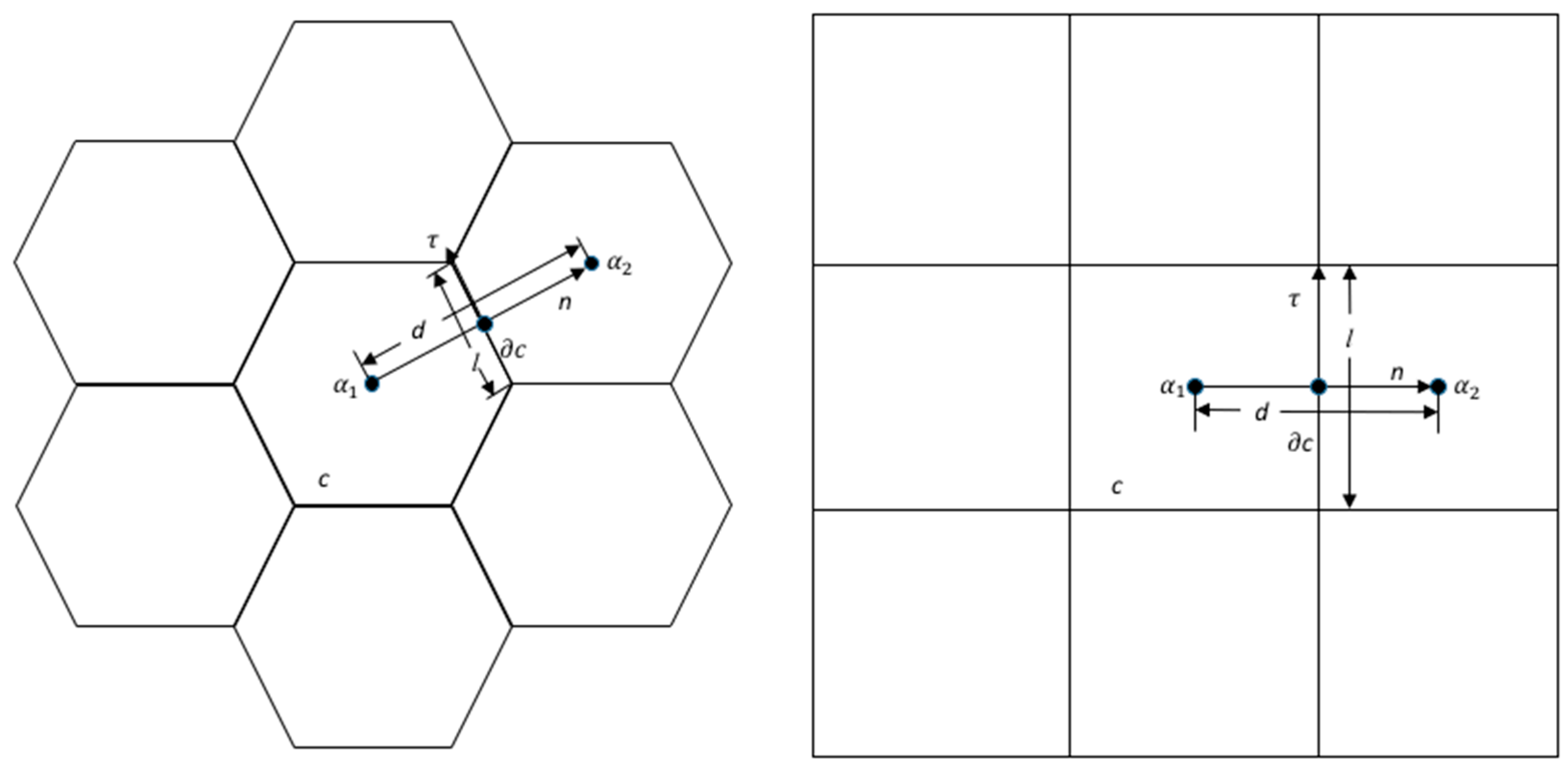
where and are arbitrary scalar functions, is any given horizontal grid cell, is the perimeter of , and and are the unit outward normal and tangential vectors, respectively, following the right-hand rule with the thumb pointing upward. In other words, Equations (1)–(3) can be solved by applying these relations repeatedly. For any given grid cell , regardless of its shape, a Voronoi Z-grid scheme places all state variables at Voronoi center , as illustrated in Figure 1.
By considering the Laplacian operator of Equation (8) as an example, we have the following approximation:
The continuous curve integral along is approximated by a set of piece-wise line integrals along surrounding cell , where runs through all edges of . These line integrals in (9) are then approximated by the directional derivatives multiplied by the edge lengths. For normal derivative , a two-stencil scheme is applied: . If all of the cells are regular (i.e., the Voronoi and centroid centers are at the same location), then this approximation can achieve second-order accuracy. To simplify the discussion, the Z-grid models are discussed for planes and the cells are assumed to be regular.
A generalization of a Voronoi Z-grid model is achieved by using a grid stencil beyond the two Voronoi centers for normal derivatives of edges in (9). On a grid of a two-dimensional plane, the second-order accurate approximation of can be ensured using a six-grid or larger stencil based on Taylor expansions, regardless of whether a Voronoi or centroid center is used. As a finite volume method defines the state variables at centroidal centers, we always choose a centroidal center in this generalized scheme regardless of whether it is used on a plane or sphere where Voronoi and centroid centers may differ. Thus, we call this scheme the centroidal Z-grid hereafter. To ensure that the generalized scheme conserves scalar quantities, the line integrals are constructed using the same stencils for two cells sharing common edges. Hence, the six-grid stencil must be symmetric on both sides of the edge. Hexagons of an icosahedral grid cannot be symmetric; thus, we divided these hexagons and pentagons into triangles. Figure 2 shows the symmetry for both triangular and rectangular grids. A convenient feature of this triangular grid on a sphere is that each cell has three edges, with each edge being associated with the six closest grid cells. Moreover, all the three edges of a cell are in the same plane. This homogeneity of the triangular grid makes parallel computing much easier, and in addition, the grid can be easily nested compared to a hexagonal/pentagonal grid.
The Voronoi Z-grid model interpolates function values at both the ends of an edge and uses a centered finite difference to approximate the tangential derivative at the edge center. For tangential derivatives, the new proposed Z-grid model applies the same stencil as the Voronoi Z-grid model for achieving second-order accuracy. For the sake of simplicity, in the current study, we used a rectangular grid for the model formulation and numerical experiments; we will discuss an icosahedral grid on a sphere in more detail in our future works.
Note that the subindex integers of 1,2,…,6 in Figure 2 serve a symbolic purpose only. For each edge, the indices are different. For a rectangular grid, the Voronoi Z-grid model approximates the line integrals of the operators of Equations (6)–(8) as follows:
For the tangential derivative, the model actually uses
and the grid values of and in (13) cancel out in Equation (10) for the rectangular grid. Thus, we showed that the model definitely uses a six-grid stencil. The proposed centroidal Z-grid uses the same stencil as that of the Voronoi Z-grid. However, the Voronoi Z-grid model uses different stencils for approximating tangential and normal derivatives. Our new generalization retains the tangential approximation and uses a six-grid stencil to approximate all the normal derivatives in the following approximations:
where , and are weights satisfying , , and , respectively, and
Parameters , , and denote the top, middle, and bottom cells on the right column of Figure 2. When and , the corresponding model reduces to the Voronoi Z-grid model shown previously. Thus, this proposed model with choices of parameters , and is a generalization of the Z-grid model. By applying Taylor expansion, we can prove that this new model is second-order accurate on a rectangular grid, possesses all conservation properties of the Voronoi Z-grid model, and provides flexibility in testing other choices of the weights. Moreover, we demonstrate that some selection of nonzero and provides more stability and can utilize longer time steps in the temporal integration of the discretized shallow water equations. Our numerical experiments showed that if satisfying (16) then the Z-grid model is stable, but a scheme of does not show stability.
3. Dispersion Relation Analysis
Before demonstrating the stability of the centroidal Z-grid, determining how this generalization affects the dispersion relation would be interesting, as it is an important feature approximating the continuous equations. We analyzed the centroidal Z-grid dispersion relation and compared it to the Voronoi Z-grid in order to have a better understanding of how the dispersion relation changes. Furthermore, the relation may provide some guidance to choosing weights , , and .
In this study, a linearized rotating shallow-water-equation system was used in the dispersion relation analysis:
To convert these equations into the Z-grid equations, we need to derive the vorticity and divergence equations. First, we applied in Equations (17) and (18) and obtained
where and . Then, by applying on these Equations, we obtained
We applied in Equation (20) to obtain
and by using (21), we have
Then, Equation (19) can be rewritten as
and used to replace the divergence in Equation (23) so that
Assume a wave solution of to have the form . By substituting this solution into Equation (25), we have
or
Let be the deformation radius of this shallow water Equation; then the dispersion relation satisfies
The three eigenvalues are represented as
and
which is the continuous dispersion relation and where is any constant. Any discrete numerical scheme should approach this relation as much as possible. The closer a scheme is to the continuous relation of Equation (28), the better is the scheme’s dispersion relation.
Now, we look into the discrete forms (10), (14), and (15) of a centroidal Z-grid model in solving Equation (20). Equation (20) mainly involves calculating a Laplacian operator. For a uniform grid with a grid spacing of in both and directions, a Z-grid model places the model states at the center of a square cell. The Z-grid model should approximate over a cell by using the Laplacian relation
where is the outward normal direction. For a cell located at , the centroidal Z-grid model uses six stencils to approximate the normal derivative. For the left edge, we have
where and satisfying (16). By assuming for the right, bottom, and top edges, we also have
Let , then
Thus, Equation of (30) and the three Equations next it become the following forms,
Therefore, the finite volume scheme gives
By assuming , and replacing in Equation (20) with this discrete form, Equation (20) is rewritten as
Further, Equation (21) gives
and Equation (19) gives
By replacing and in the abovementioned spectral Equation, we have
or
For the given relation and assuming that , we can find optimal weights that minimize the difference between Equations (28) and (31) in norm. Over the region , the optimal weights are close to and , which possess an even better dispersion relation than the Voronoi Z-grid. However, we found that these optimal weights could result in an unstable model. Thus, we determined to seek weights that provided stability and the best possible dispersion relation.
To determine the difference between the continuous and discrete dispersion relations, we calculated the difference between the right hand sides of Equations (28) and (31) as functions of over three domains from the origin through 1) ; 2) ; and 3) and . We compared three typical centroidal Z-grids with weights selected as (, ), (, ), and (, ) to the Voronoi Z-grid. The differences between Equations (28) and (31) over these three domains are shown in Table 1.
This table shows that there is a better choice of weights than those possessed by the Voronoi Z-grid as they give a better dispersion relation (, ). We also found in our numerical experiments that, with this choice of weights, the centroidal Z-grid is as stable as the Voronoi Z-grid. Thus, for the centroidal Z-grid models, we can choose weights such that their dispersion relation is as good as possible and provides more stability.
4. Modification of the Test Cases
To show the stability of the centroidal Z-grid, we chose two typical test cases for shallow water equations: the Rossby–Haurwitz [11] and Galewsky [12] test cases. We modified these cases to fit our numerical experiments over a rectangular grid simulating a global latitudinal/longitudinal grid.
The Rossby–Haurwitz test case is used for testing various models, including spectral and gridded models, because of its realism and nonlinear instability that closely reflect the real atmosphere. The stream function in this case provides a realistic wave pattern around a globe, and we extended it in this study to make the stream function move with time as follows:
where is the radius of the Earth; is the latitude; is the longitude; , are constants and is an integer constant; and is the time in seconds. This stream function moves from west to east at an angular velocity given by the following Equation:
where is the rotational angular velocity of the Earth. This is a divergence-free test case, that is, and . We adapted it to a latitudinal/longitudinal plane for testing the numerical accuracy and stability of the centroidal Z-grid scheme. However, this test case (Williamson et al. [11]) does not satisfy the continuous shallow water Equations (1)–(5). A common practice is to compare a given model output to the numerical output produced through a spectral model that solves the dissipative shallow water equations by using an appropriate initial condition (e.g., [4]). A dissipation was used in a spectral model to control noise from high-frequency waves. Such a comparison may not serve our purpose, as we need to know the stability of our Z-grid models. A diffusive solution may not be able to demonstrate the differences of these Z-grid models. Hence, we attempted to search for a non-diffusive solution to check the stability of our model for the Rossby–Haurwitz case.
We selected a method suggested by Browning et al. [13]. This method adds forcing terms to a given system of equations to force a Rossby–Haurwitz case to become the exact solution for the non-diffusive shallow water Equations (1)–(5). For our test on the latitudinal/longitudinal plane, we used the Rossby–Haurwitz stream function in Equation (32) and chose the fluid depth such that the divergence Equation (2) was satisfied perfectly. In other words, by substituting , , and in Equations (2) and (5), we solved , satisfying the following:
By choosing in such a manner, Equation (2) is satisfied, and no forcing term is required for Equation (2). We then applied the stream function given by Equation (32), its corresponding vorticity , and fluid depth that satisfies Equation (34) into Equations (1) and (3) and obtained two forcing functions, denoted as and . Then, the functions , , and solution of Equation (34) satisfy the following non-diffusive Equations:
Our numerical forecast results can be verified against this true solution at any given time to demonstrate the stability and efficiency of the centroidal and Voronoi Z-grid models.
This modification methodology for shallow-water-equation test cases can also be applied to the Rossby–Haurwitz test case on a sphere. The only difference is that the differential operators will be spherical and not Cartesian in the latitudinal and longitudinal directions. A similar process can also be applied to other test cases of shallow water equations. However, the Rossby–Haurwitz case is a very challenging case because of its nonlinearity. Hence, the comparison of the stability of both the models is sufficient.
Note that Equation (34) may be too complicated to solve for an analytic solution of . Instead, for any given resolution and time in our numerical experiments, we solved Equation (34) numerically.
To test a regional Z-grid model, we must specify the boundary conditions. In general, a global or larger domain model provides Dirichlet boundary conditions to a regional Z-grid model. For the Rossby–Haurwitz test case, we chose a latitudinal and longitudinal domain and considered the east–west boundaries as periodic boundaries, thereby simulating a global latitudinal and longitudinal grid and using the Dirichlet boundary conditions at the north and south boundaries from the continuous solution of this test case.
Numerical noise usually appears near the Dirichlet boundaries because the boundary values do not match the predicted values of the model due to truncation errors, even though these errors are very small. A sponge boundary treatment [14] is usually used to minimize the spurious wave reflections. In our implementation of the Z-grid models, we used a simple sponge method to avoid the spurious reflections at the north and south boundaries. We used the true boundary values and forecast grid values at the second interior to interpolate the grid values at the first interior next to the boundaries (hereafter referred to as the averaging boundary conditions). This method removes boundary reflections without loss of model accuracy. Therefore, we applied this averaging boundary condition throughout our numerical experiments.
The Galewsky test case was also modified to fit our numerical experiments over a rectangular domain. We kept the zonal flow formulation obtained from [12],
and the perturbation field,
where ms−1, , , , , , , and m. Instead of using the height field in [12], we solved Equation (34) as well to obtain a balanced height field for the background flow given by Galewsky et al. [12]. We modified the derivative operators in (34) as a rectangular grid coordinate of so that the Equation for the height field has the following form:
A mean constant height, m, was added to the solution of (40) so that the mean average height was around 10 km, as suggested by Galewsky et al. [12]. All the partial derivatives were treated as a Cartesian coordinate of instead of a spherical coordinate.
5. Numerical Experiments
As stated earlier, a multigrid technique is usually applied in Z-grid models for solving the Poisson Equations in (4), converting vorticity and divergence to a stream function and velocity potential, respectively. For an accurate comparison between the centroidal and Voronoi Z-grid models, we used FISHPACK [15] in our regional Z-grid model experiments. This is not an iterative method but solves Poisson equations numerically with second-order accuracy. However, this solver is not sufficiently efficient to implement a Z-grid model in general. By using this solver, we avoid clarifying the implementation of a multigrid method and its convergence solving the Poisson equations numerically. Given that our goal is to show the improved stability and longer time step integration of the new Z-grid model, FISHPACK is appropriate.
The FISHPACK solver enables us to specify the Dirichlet boundary conditions at the north and south boundaries, and periodic boundary conditions at the east and west boundaries. Our domain involves the latitudinal and longitudinal grids of the whole globe, and these boundary conditions meet our needs. For all numerical experiments presented herein, the same solver was used for all Z-grid-model comparisons.
We implemented three Z-grid models to demonstrate the improvement of the new Z-grid model. For the Voronoi Z-grid model, we used the finite volume scheme defined by Equations (10), (14), and (15) by setting and , denoted as VORO (Voronoi scheme) hereafter. For the new centroidal Z-grid model, we used and ; this scheme is denoted as CENT. We also chose the centroidal Z-grid with the “best” dispersion relation, with and and denoted it as BEST.
In our experiments, we chose parameters for the Rossby–Haurwitz test case. Other physical parameters used in the experiments of both cases were as follows: , , and .
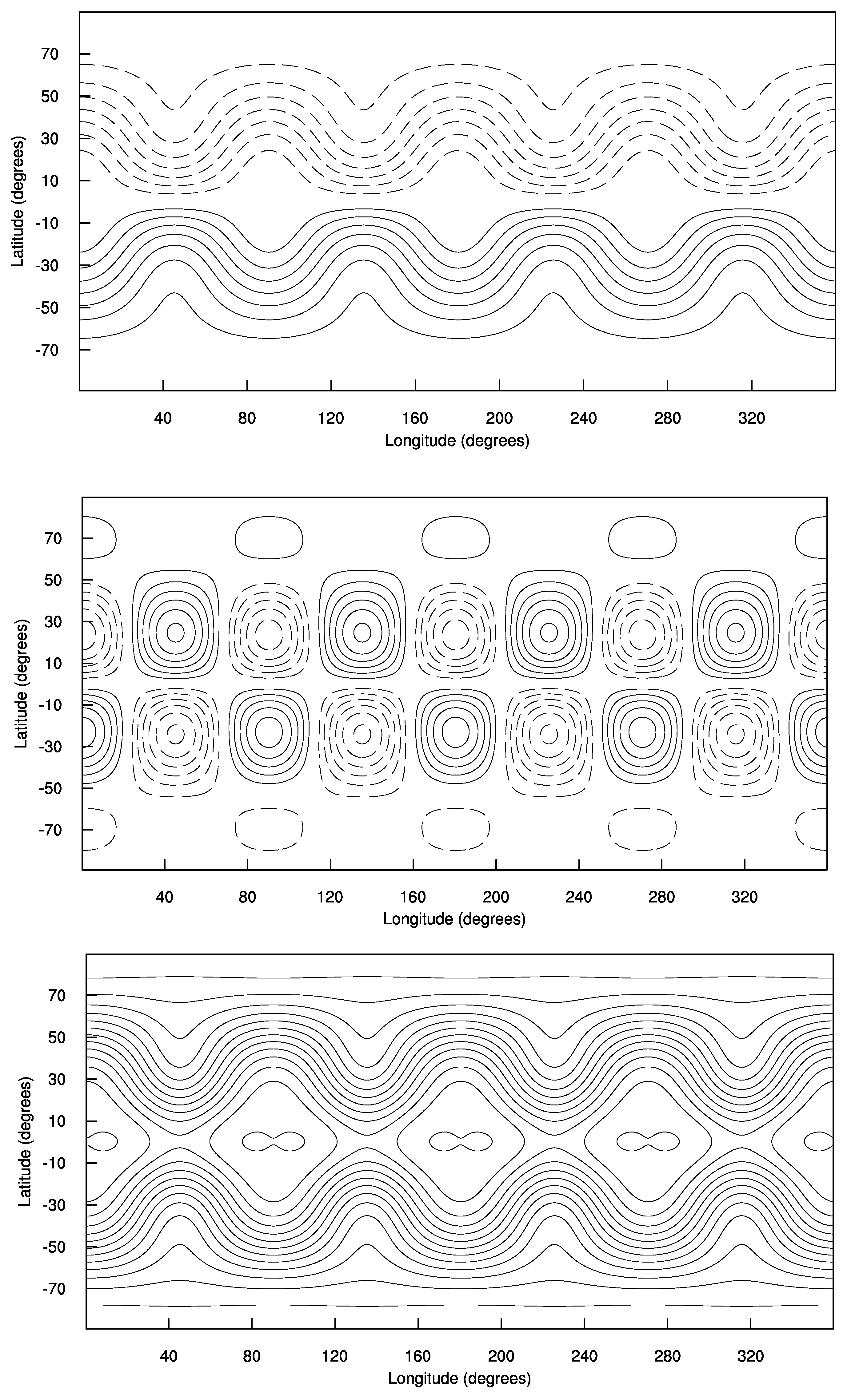
Figure 3 shows the stream function given by Equation (32), along with its absolute vorticity and fluid depth of the continuous Rossby–Haurwitz test case on the latitudinal/longitudinal plane in a one-degree resolution. For the Galewsky case, the background flow is given in Equations (38) and the solution of (40) and the perturbation (39) is shown in [12].
For the time integration of our numerical experiments, we used a Runge–Kutta fourth-order scheme, even though it is relatively expensive compared to the third-order Adams–Bashforth scheme [16]. Both Runge–Kutta and Adams–Bashforth schemes are classified as Eulerian-based time-integration (EBIT) schemes [17]. They are sufficient to support the numerical experiments in this study. The Runge–Kutta fourth-order scheme is free of a computational mode and is less diffusive. It serves the purpose of comparing the model stability well. An Adams–Bashforth scheme or some path-based time-integration (PBTI) schemes [17] will be implemented in practical applications.
All numerical experiments in this Rossby–Haurwitz case are free of any numerical dissipation. Even though Galewsky et al. [12] suggested a second-order dissipative for all equations, we applied a second-order dissipation to the vorticity and divergence Equations (1) and (2) only and no numerical diffusion for (3) for the Galewsky case. The dissipation in vorticity equation is sufficiently small to remove unresolvable noise. For each model, we tried several time step lengths until the longest one was found for stability. For the Rossby–Haurwitz case, the numerical forecast ran for 14 days and for the Galewsky case, it ran for 6 days, the same as in [12]. The time step used by the CENT scheme can be as much as 1.4 times that of the VORO and BEST schemes for the Rossby–Haurwitz case and 1.6 times for the Galewsky case. For example, at a one-degree resolution, the CENT scheme can take a time step of 840 s but VORO took just 600 s for the Rossby–Haurwitz case; CENT can take one of 480 s but VORO took just 300 s for the Galewsky case. These longer time-integration steps of CENT are indeed significant. The computer runtime confirms the efficiency improvement. For the Rossby–Haurwitz case, the runtime is shown in Figure 4 with three different resolutions. Computing time is saved significantly as the resolutions increase.
As we know the exact solution of the forced shallow-water Equations for the Rossby–Haurwitz case, we calculated the errors against the true solution of at the end of the 14th day in two error norms: and . In the error table (Table 2), the -norm error is a relative error and is defined as
and norm error is the maximum error over the domain and is given as
where is an index for all grid cells over a given domain. We reported the results in to show that error reduction is everywhere over the domain as expected for a second-order scheme, indicating that our implementation of these schemes was correct. Table 2 lists the 14th-day forecast errors of the Rossby–Haurwitz case at two-, one-, and half-degree resolutions against the true solution of the forced shallow water Equations (35)–(37).
The error reduction from coarse to one-level-finer resolutions is close to a factor of four, which matches the second-order accuracy expectation of these models over the rectangular latitudinal and longitudinal grids. Notably, the maximum errors in are also reduced by a factor of four. This study numerically showed that the schemes are second-order accurate anywhere in the domain and the numerical results reflect the correctness of the implementation. At a resolution of one degree, these models have relative errors less than 5% and 0.6% in terms of vorticity and fluid depth, respectively. Thus, the forecast fields are visually identical to those in Figure 3 and do not need to be plotted (the forecast error of vorticity is plotted in Figure 5).
By applying the averaged boundary conditions introduced in the previous section, we found that the spurious reflection was removed completely. Figure 6 shows a north–south cross-section of the 14th-day vorticity forecast at a longitude of 40° when using the CENT scheme. No noise was observed near the south and north boundary grids, which are labeled near grid indices of −90 (south) and 90 degree (north). The maximum error reductions given in Table 2 indicate that these averaging boundary conditions properly maintain the model accuracy for both the CENT and VORO Z-grid schemes.
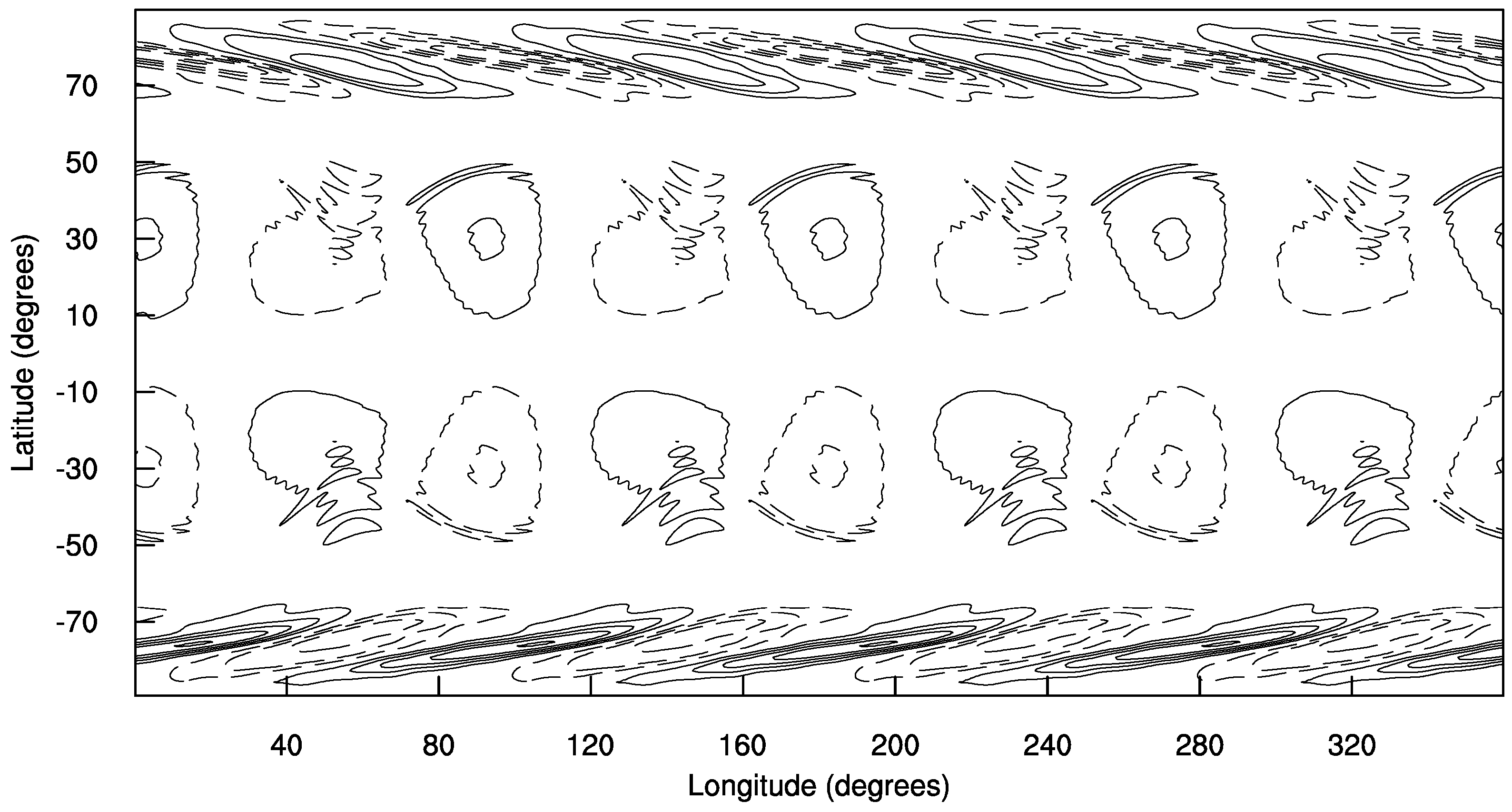
For the Galewsky test case, Figure 7 and Figure 8 show the numerical forecasts of the vorticity and absolute vorticity at 96 h, 120 h, and 144 h. Compared to Figure 4 in [12], these figures closely resemble the features at all these hours. Thus, these Z-grid models performed appropriately and reasonably reflected the unstable jet over an isolated mountain. These models produced almost identical plots, and we thus obtained the numerical results from the CENT model’s half-degree resolution outputs.
In summary, we found that the centroidal Z-grid model could utilize time steps that are at least 1.4 times or longer in all of the resolutions for both test cases in this study. Of course, these longer time steps reduce the computing time by 30% or more at half-degree runs.
Note that our numerical experiments are based on the sequential codes of these Z-grid models. The runtime is a single-processor forecast time. As the models are almost identical, this computing-time reduction will certainly hold in a massively parallel computing environment. That is, a more than 30% efficiency improvement of the new model can also be achieved in parallel computing environments.
The new centroidal Z-grid model comprises more grid values used for the normal derivatives, and these may affect efficiency. It is indeed a minor addition as this happens only for calculation of the normal derivatives. Furthermore, the Poisson solver uses the majority of the computing time, even though a multigrid technique is used. For massive parallel computing, the computing involving a large number of grid values is of less concern. Model stability is beneficial in that it is significantly more viable for longer time-integration steps.
6. Conclusions and Remarks
A generalized Z-grid model was proposed and tested in comparison to the Voronoi Z-grid model. The proposed model has improved stability and efficiency. The comparison showed that the new centroidal model reduces the computation time by more than 30% compared to the Voronoi Z-grid model, while retaining the good features of a Voronoi Z-grid model, thus being more efficient. In addition, the small forecast errors at the end of the 14th day show that the centroidal model did not result in much energy loss while conserving all of the scalar variables, such as momentum, divergence, and vorticity, as well as mass fields.
For the weights of the centroidal Z-grid models, we tested different options. Specifically, we found that weights and were more stable than others on rectangular grids, maintaining relatively good dispersion relations. The numerical experiments were performed on a rectangular domain; however, we expect that a similar conclusion would be obtained for global icosahedral triangular Z-grid models. The regional domains of a plane and sphere differ with respect to the continuous spherical derivative operators; this will result in different coefficients of the shallow water equations. In our future study, we will focus on the centroidal Z-grid models with respect to a sphere.
The modification of the Rossby–Haurwitz test case and the methodology of this modification can be applied on a sphere and other test cases of shallow water equations. The advantage of this methodology is that it does not rely on the numerical solutions of a spectral model, and thus enables users to perform a clean comparison to the true solution. However, the realism of adding forcing functions to the governing equations may be of concern. To address this issue, it must be noted that in reality, forecast models or their equations are affected by the radiation of the Sun, for example, along with other physical forces. Hence, having test cases that satisfy the forced shallow water equations is reasonable.
Regarding time-integration schemes, the use of the Runge–Kutta fourth-order scheme in this study was mainly considered for stability comparison. In Z-grid model applications, a third-order Adams–Bashforth or other PBTI methods are more practical for saving computing time.
Funding
This work is supported by the National Basic Research and Development Program of China (2017YFC1502201), and the Basic Scientific Research and Operation Foundation of the CAMS (Grant No. 2017Z017).
Acknowledgments
The author would like to thank the two anonymous reviewers for their careful reviews and suggestions on improving the presentation and numerical experiments of this paper.
Conflicts of Interest
The author declares no conflicts of interest.
References
- Adcroft, A.J.; Hill, C.N.; Marshall, J.C. A new treatment of the Coriolis terms in C-Grid models at both high and low resolutions. Mon. Weather Rev. 1999, 127, 1928–1936. [Google Scholar] [CrossRef]
- Tomita, H.; Tsugawa, M.; Satoh, M.; Goto, K. Shallow water model on a modified icosahedral geodesic grid by using spring dynamics. J. Comput. Phys. 2001, 174, 579–613. [Google Scholar] [CrossRef]
- Thuburn, J.; Ringler, T.D.; Skamarock, W.C.; Klemp, J.B. Numerical representation of geostrophic modes on arbitrarily structured C-grids. J. Comput. Phys. 2009, 228, 8321–8335. [Google Scholar] [CrossRef]
- Ringler, T.; Thuburn, J.; Klemp, J.; Skamarock, W. A unified approach to energy conservation and potential vorticity dynamics for arbitrarily structured C-grids. J. Comput. Phys. 2010, 229, 3065–3090. [Google Scholar] [CrossRef]
- Lin, S.-J.; Rood, R.B. An explicit flux-form semi-Lagrangian shallow-water model on the sphere. Q. J. R. Meteorol. Soc. 1997, 123, 2477–2498. [Google Scholar] [CrossRef]
- Heikes, R.P.; Randall, D.A. Numerical Integration of the shallow-water equations on a twisted icosahedral grid, Part I: Basic design and results of tests. Mon. Weather Rev. 1995, 123, 1862–1880. [Google Scholar] [CrossRef]
- Randall, D. Geostrophic adjustment and the finite difference shallow water equations. Mon. Weather Rev. 1994, 122, 1371–1377. [Google Scholar] [CrossRef]
- Heikes, R.P.; Randall, D.A.; Konor, C.S. Optimized icosahedral grids: Performance of finite-difference operators and multigrid solver. Mon. Weather Rev. 2013, 141, 4450–4469. [Google Scholar] [CrossRef]
- Briggs, W.L.; Henson, V.E.; McCormick, S.F. A Multigrid Tutorial, 2nd ed.; SIAM: Philadelphia, PA, USA, 2000. [Google Scholar]
- Eldred, C.; Randall, D. Total energy and potential enstrophy conserving schemes for the shallow water equations using Hamiltonian methods—Part 1: Derivation and properties. Geosci. Model. Dev. 2017, 10, 791–810. [Google Scholar] [CrossRef]
- Williamson, D.L.; Drake, J.B.; Hack, J.J.; Jacob, R.; Swarztrauber, P.N. A standard test set for numerical approximations to the shallow water equations in spherical geometry. J. Comput. Phys. 1992, 102, 211–224. [Google Scholar] [CrossRef]
- Galewsky, J.; Scott, R.K.; Polvani, L.M. An initial value problem for testing numerical models of the global shallow water equations. Tellus A 2004, 56, 429–440. [Google Scholar] [CrossRef]
- Browning, G.L.; Hack, J.J.; Swarztrauber, P.N. A comparison of three numerical methods for solving differential equations on the sphere. Mon. Weather Rev. 1989, 117, 1058–1075. [Google Scholar] [CrossRef]
- Kar, S.K.; Turco, R.P. Formulation of a lateral sponge layer for limited-area shallow-water models and an extension for the vertical stratified case. Mon. Weather Rev. 1995, 123, 1542–1559. [Google Scholar] [CrossRef]
- Sweet, R.A. Cyclic reduction algorithm for solving block tridiagonal systems of arbitrary dimensions. SIAM J. Numer. Anal. 1977, 14, 706–720. [Google Scholar] [CrossRef]
- Durran, D.R. The third-order Adams-Bashforth method: An attractive alternative to leapfrog time differencing. Mon. Weather Rev. 1991, 119, 702–720. [Google Scholar] [CrossRef]
- Mengaldo, G.; Wyszogrodzki, A.; Diamantakis, M.; Lock, S.J.; Giraldo, F.X.; Wedi, N.P. Current and Emerging Time-Integration Strategies in Global Numerical Weather and Climate Prediction. Arch. Comput. Methods Eng. 2018. [Google Scholar] [CrossRef]
Figure 1.
Voronoi Z-grid finite volume scheme for different grid cells.

Figure 2.
Six-stencil centroidal Z-grid model.

Figure 3.
Continuous stream function (top), vorticity (middle), and fluid depth (bottom) at a one-degree resolution. Stream function is in the range of (−3 × 10⁸, 3 × 10⁸), vorticity in (−6 × 10⁻⁵, 6 × 10⁻⁵), and depth in (600, 3000).
Figure 3.
Continuous stream function (top), vorticity (middle), and fluid depth (bottom) at a one-degree resolution. Stream function is in the range of (−3 × 10⁸, 3 × 10⁸), vorticity in (−6 × 10⁻⁵, 6 × 10⁻⁵), and depth in (600, 3000).

Figure 4.
Computer runtime in seconds for the Rossby–Haurwitz case: 1. two-degree resolution; 2. one-degree resolution; and 3. half-degree resolution. CENT, centroidal; VORO, Voronoi; BEST, best.
Figure 4.
Computer runtime in seconds for the Rossby–Haurwitz case: 1. two-degree resolution; 2. one-degree resolution; and 3. half-degree resolution. CENT, centroidal; VORO, Voronoi; BEST, best.

Figure 5.
Forecast error of vorticity on the 14th day of the CENT model at half-degree resolution. Error sizes are in the range of (−10−7, 10−7).
Figure 5.
Forecast error of vorticity on the 14th day of the CENT model at half-degree resolution. Error sizes are in the range of (−10−7, 10−7).

Figure 6.
North–south cross-section of the vorticity errors at 40° longitude.

Figure 7.
Vorticity forecasts at 96 h (top), 120 h (middle), and 144 h (bottom).

Figure 8.
Absolute vorticity forecasts at 96 h (top), 120 h (middle), and 144 h (bottom).


Table 1.
Dispersion relation difference between discrete and continuous dispersion relations.
| Radius | Voronoi Z-Grid | Centroidal Z-Grid (0.5, 0.25) | Centroidal Z-Grid (0.75, 0.125) | Centroidal Z-Grid (1.02, −0.01) |
|---|---|---|---|---|
| 0.113 | 0.307 | 0.207 | 0.106 | |
| 0.887 | 1.957 | 1.358 | 0.854 | |
| 1.199 | 2.927 | 1.910 | 1.150 |
Table 2.
Forecast errors on the 14th day of the two Z-grid models of CENT, VORO and BEST.
| Errors | () | () | () |
|---|---|---|---|
| CENT (2o) | 0.1884 × 10⁻¹/ | 0.1233 × 10⁶/ | 0.2518 × 10⁻²/ |
| 0.1661 × 10⁻⁵ | 0.4392 × 10⁻⁶ | 0.1067 × 10² | |
| VORO (2o) | 0.1818 × 10⁻¹/ | 0.7939 × 10⁻⁷/ | 0.2373 × 10⁻²/ |
| 0.1628 × 10⁻⁵ | 0.4392 × 10⁻⁶ | 0.1051 × 10² | |
| BEST (2o) | 0.1814 × 101/ | 0.7664 × 10⁻⁷/ | 0.2364 × 10⁻²/ |
| 0.1628 × 10⁻⁵ | 0.4362 × 10⁻⁶ | 0.1050 × 10² | |
| CENT (1o) | 0.4786 × 10⁻²/ | 0.3480 × 10⁻⁷/ | 0.6335 × 10⁻³/ |
| 0.4576 × 10⁻⁶ | 0.1274 × 10⁻⁶ | 0.2721 × 101 | |
| VORO (1o) | 0.4516 × 10⁻²/ | 0.2169 × 10⁻⁷/ | 0.5979 × 10⁻³/ |
| 0.4302 × 10⁻⁶ | 0.9216 × 10⁻⁷ | 0.2667 × 101 | |
| BEST (1o) | 0.4494 × 10⁻²/ | 0.2118 × 10⁻⁷/ | 0.5957 × 10⁻³/ |
| 0.4278 × 10⁻⁶ | 0.8718 × 10⁻⁷ | 0.2668 × 101 | |
| CENT (0.5o) | 0.1185 × 10⁻²/ | 0.9465 × 10⁻⁸/ | 0.1588 × 10⁻³/ |
| 0.1164 × 10⁻⁶ | 0.4072 × 10⁻⁷ | 0.6603 × 100 | |
| VORO (0.5o) | 0.1120 × 10⁻²/ | 0.5632 × 10⁻⁸/ | 0.1500 × 10⁻³/ |
| 0.1051 × 10⁻⁶ | 0.2003 × 10⁻⁷ | 0.6625 × 100 | |
| BEST (0.5o) | 0.1116 × 10⁻²/ | 0.5464 × 10⁻⁸/ | 0.1495 × 10⁻³/ |
| 0.1042 × 10⁻⁶ | 0.1971 × 10⁻⁷ | 0.6631 × 100 |
© 2019 by the author. Licensee MDPI, Basel, Switzerland. This article is an open access article distributed under the terms and conditions of the Creative Commons Attribution (CC BY) license (http://creativecommons.org/licenses/by/4.0/).
Share and Cite
MDPI and ACS Style
Xie, Y. Generalized Z-Grid Model for Numerical Weather Prediction. Atmosphere 2019, 10, 179. https://doi.org/10.3390/atmos10040179
AMA Style
Xie Y. Generalized Z-Grid Model for Numerical Weather Prediction. Atmosphere. 2019; 10(4):179. https://doi.org/10.3390/atmos10040179
Chicago/Turabian StyleXie, Yuanfu. 2019. "Generalized Z-Grid Model for Numerical Weather Prediction" Atmosphere 10, no. 4: 179. https://doi.org/10.3390/atmos10040179
Note that from the first issue of 2016, this journal uses article numbers instead of page numbers. See further details here.