Optimization of Parameters in the Generalized Extreme-Value Distribution Type 1 for Three Populations Using Harmonic Search

Abstract

Due to its geographical position, Mexico is exposed annually to cold fronts and tropical cyclones, registering extremely high values that are atypical in the series of maximum annual flows. Univariate mixed probability distribution functions have been developed based on the theory of extreme values, which require techniques to determine their parameters. Therefore, this paper explores a function that considers three populations to analyze maximum annual flows. According to the structure of the Generalized Extreme-Value Distribution (GEV), the simultaneous definition of nine parameters is required: three of location, three of scale, and three of probability of occurrence. Thus, the use of a meta-heuristic technique was proposed (harmonic search). The precision of the adjustment was increased through the optimization of the parameters, and with it came a reduction in the uncertainty of the forecast, particularly for cyclonic events. It is concluded that the use of an extreme value distribution (Type I) structured with three populations and accompanied by the technique of harmonic search improves the performance in respect to classic techniques for the determination of its parameters.

1. Introduction

Mathematical modeling of natural phenomena has become increasingly important due to the implications of global warming and associated climate modification, taking special relevance in public safety activities and economic aspects [1].

The modeling of extreme events is of great importance in countries affected by hurricanes. Countries in Asia and Latin America are affected by cyclones and hurricanes, therefore new approaches to frequency analysis with extreme data sets are often sought. In Mexico, a case of two hurricanes occurring simultaneously on both coasts (Ingrid and Manuel in 2013) has already presented itself. In general, hurricane winds affect infrastructure in urban areas. However, in Latin American countries, human settlements on riverbanks are very common. Material damage and loss of human life happens in rivers and their floodplains. For this reason, this paper considers the evolution of maximum flows within a region highly exposed to hurricanes. This work also creates the possibility that with the proposed methodology, other climatic variables can be studied.

Regarding frequency analysis, particularly for extreme events, the objective is to define the events associated with a return period that provide information to carry out the design of hydraulic works, decreasing the uncertainty of the forecast [2].

The development of the theory of extreme values comes from the past century, with an intense exploration of applications to different disciplinary areas in the last 30 years. This theory allows the modeling of queues in distribution and can extrapolate information in extreme regions with little or no information [3]. Applications have been developed in hydrology, climatology, oceanography, and environment within the engineering area. Certainly, one of the most important applications in Mexico with regard to extreme values theory is the study of hurricane rains. There are historical data of 350 mm of cumulative rain in 24 h for hurricane Gilberto (1988) and 411 mm (948 mb) in 24 h for hurricane Paulina (1997), two of the most destructive hurricanes that have ever hit Mexico [4]. These kinds of events are certainly extreme rainfall if compared with the national mean of 770 mm per year. A detailed study of the origin, characteristics, properties, and applications in hydrology for the function of the Generalized Extreme-Value Distribution (GEV) was presented in Mexico [5,6].

The study of 31 historical records of flows, maximum annual precipitation, and maximum wind speeds obtained in rivers and regions of Canada, the United States, England, Kenya, Mexico, New Zealand, and Switzerland was carried out using the GEV distribution, comparing its performance using the expressions of standard error and absolute error of adjustment [7].

The graphical, Log-Pearson III, and Gumbel methods were applied to obtain maximum rainfall intensities in pluviographic stations in eastern Venezuela, concluding that Gumbel’s methodology is applicable for periods less than 25 years [8].

The existence of areas in which the distribution of extreme values for extra-tropical winds presents two populations, where local winds may be the product of two different systems with different physical origins [9]. Each system has its own distribution function, so we can speak of mixed functions in the modeling of information from two populations [10].

The presence of cold fronts or tropical cyclones generates atypical values in the series of maximum annual flows (Q) registered by hydrometric stations installed in the study basins [2]. This behavior has been studied using the Gumbel probability distribution function of two populations (EV1-2P) [11], which later gave rise to the development of a new type of probability function named the mixed probability distribution function [12].

Considering the statistical analysis of the record of maximum annual scale readings of a hydrometric station in southeastern Mexico, it was concluded that the Gumbel double distribution function carried out the best adjustment. The same result was obtained for the maximum annual instantaneous flows that coincide on the same timescale [13].

The proposal to use a probability distribution function based on the Type I Generalized Extreme-Value Distribution, considering three populations in records for Q [14], showed the pertinence of its application in the hydrological area and the determination of the parameters through the use of maximum likelihood (ML) methodology.

Continuing with the proposal [15] has led to a new study using the generalized extreme value distribution considering three populations for events of a different nature recorded in the same place. The parameters were determined in an analogous way using ML, and the results show a better performance when including the Type I Generalized Extreme-Value Distribution for three populations (EV1-3P).

The estimation of the parameters in the GEV has been carried out by using ML, moments, L moments, the sextiles techniques, and optimizing the objective function [7]. Multiple methods for estimating the parameters of the Gumbel distribution function are reported in the literature, with the moments and ML methods being the best known and most used of them all [16].

The incorporation of technology in hydrological studies, specifically in frequency distribution analyses, has allowed the exploration of the use of genetic algorithms [2] and meta-heuristic techniques [17].

The harmonic search (HS) method was proposed based on the principles that underlie the harmonic improvisation performed by musicians [18]; the characteristics that distinguish this algorithm are its simple and efficient structure to perform the search [19]. It has been used in areas such as the optimization of drinking water networks [20], the design of mechanical structures [21], the optimization of functions [22], and optimization in data classification systems [23].

Other application areas are industry [24,25,26,27], optimization testing [28], power systems [29,30,31], and signal and image processing [32,33], demonstrating its versatility in multiple disciplinary areas.

The exploration of HS implementation in hydrology has led to parameter estimation in the nonlinear Muskingum model [34], in the same model using a hybrid algorithm [35], in optimal groundwater remediation designs [36], in the optimization of storage operation [37], the estimation of design storms [38], the conceptual modeling of rain-runoff transformation considering seasonal variations [39], the estimation of time of concentration in basins [40], and the adjustment of Extreme Value Distribution (Type I) for two populations in series of annual maximum flows [17].

The uncertainty of the forecast is mainly associated with the size of the sample of available events, however the function adopted for its representation and the technique used to define its parameters have a substantial influence on said value. Therefore, the objective is to explore the use of the meta-heuristic technique HS in the simultaneous optimization of the necessary parameters in the EV1-3P in I time series.

2. Data and Methods

2.1. Hydrometric Data at Hydrologic Region 10

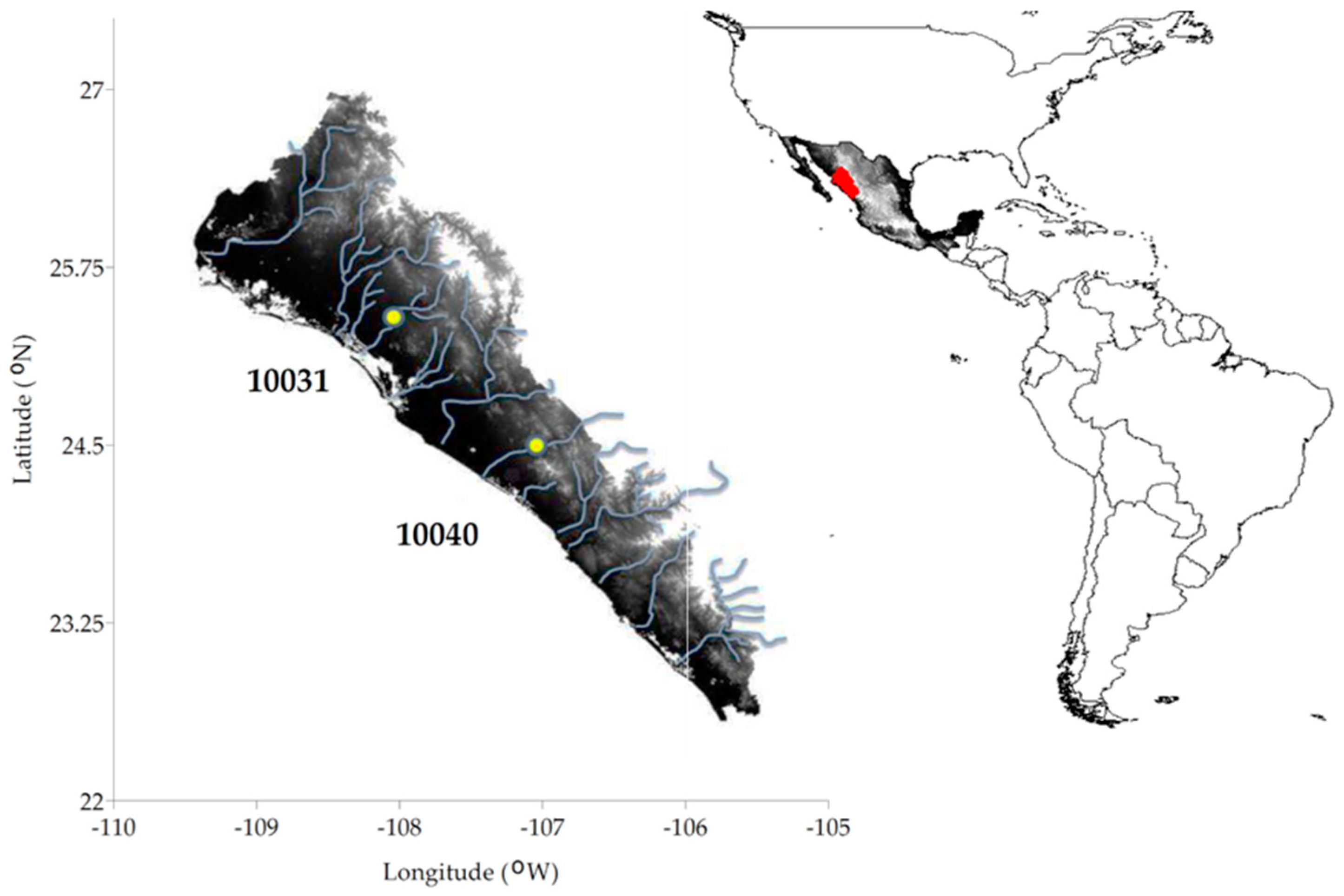
Hydrologic region 10 is located in northwest of Mexico. It extends over parts of the states of Sinaloa, Sonora, and Chihuahua, from the coastal plain to the crest of the Sierra Madre. Its area is more than 80,000 km²; it includes some rivers, which supply water for some irrigation districts and provide hydroelectric power. More than 90 gauged stations with 50 years of historical data constitute the gaging network. Hydrologic region 10 has a sub-tropical climate. A large proportion of variability in the rainfall regime of this region is due to the influence of the relief, i.e., the region is under the influence of the Sierra Madre and is exposed to what is known as the “Mexican Tropical Front”. The mean annual precipitation in this region is 800 mm, close to the national average (770 mm). The rainy season in this region is between June and October. However, long periods of drought and long periods of flood have been recorded, induced mainly by extreme meteorological phenomena. This is a sensitive region exposed to climatic changes.

To carry out the comparison of the parameters obtained for the EV1-3P using the classical ML technique with respect to the meta-heuristic HS technique, low records (Q) from the hydrometric stations of Santa Cruz (10040) and Guamuchil (10031) were used.

Gaging station 10040 is located in the San Lorenzo River, at the coordinates 24°29′05″ N and 106°57′10″ W, and measures flows over a catchment area of 8919 km². It is placed 24 km upstream of the federal highway #15 bridge on the Mazatlan–Culiacan route, near Santa Cruz de Alaya, in the municipality of Cosala. Gaging station 10031 is located over the Mocorito River, at the coordinates 25°28′10″ N and 108°05′10″ W, and measures flows over a catchment area of 1645 km². It is placed at the crossroads between the river and the South Pacific railroad, on the northern side of the city of Guamuchil. The gaging stations are in the state of Sonora (Figure 1), and their information was consulted in the National Data Bank of Surface Waters (BANDAS acronym in Spanish) through the official website of the National Water Commission (CONAGUA acronym in Spanish). In Mexico, hydrometric measurements are performed with Mexican Standards (NMX) produced by CONAGUA. These Mexican standards are based on ASTM D3858-95 and ASTM D5130-95. The stability of the cross-sectional area is verified twice a year by CONAGUA. The homogeneity of the database is reviewed annually by the Mexican Institute of Water Technology (IMTA).

The hydrometric data was extracted from the maximum annual flows of the sample of the mean daily flows at each station. Precautions were taken at all times not to select the annual instantaneous maximum values measured at the stations; this in accordance with the theory of extreme values because only one value is being sampled.

The historical Q series considered for station 10040 has 45 data points (

Table 1. Maximum annual flows recorded at hydrometric station 10040.

Year	Q (m3/s)	Year	Q (m3/s)	Year	Q (m3 s–1)	Year	Q (m3/s)
1943	2103.0	1955	1252.0	1967	950.0	1979	3080.0
1944	2142.0	1956	369.5	1968	7000.0	1980	1550.0
1945	1023.4	1957	330.0	1969	484.0	1981	306.2
1946	837.6	1958	1958.0	1970	920.6	1982	151.0
1947	1161.2	1959	762.2	1971	812.0	1983	83.0
1948	1062.0	1960	1074.0	1972	3332.4	1984	126.0
1949	784.2	1961	1280.0	1973	898.0	1985	875.0
1950	1086.3	1962	1002.0	1974	2790.0	1986	608.2
1951	487.8	1963	3680.0	1975	620.0	1987	134.1
1952	677.0	1964	861.0	1976	1495.0
1953	807.0	1965	888.8	1977	836.0
1954	553.0	1966	1166.4	1978	940.0

), while station 10031 consists of 37 data points (

Table 2. Maximum annual flows recorded at hydrometric station 10031.

Year	Q (m3/s)	Year	Q (m3/s)	Year	Q (m3/s)	Year	Q (m3/s)
1938	35.0	1948	648.0	1958	1014.0	1968	200.0
1939	299.0	1949	375.0	1959	1610.0	1969	312.0
1940	254.5	1950	272.3	1960	137.0	1970	520.0
1941	65.3	1951	422.3	1961	524.5	1971	1045.0
1942	445.0	1952	376.8	1962	985.0	1972	33.8
1943	1550.0	1953	1173.0	1963	459.5	1973	12.5
1944	391.8	1954	219.0	1964	390.0	1974	10.5
1945	916.0	1955	3507.0	1965	449.0
1946	241.0	1956	165.0	1966	793.9
1947	530.0	1957	526.0	1967	719.5

). This was to establish the frame of comparison with the studies carried out by Raynal and Garcia [14].

Subsequently, the Q register was ordered in a decreasing way, assigning to each annual flow a period of return in accordance with the expression proposed by Weibull (Equation (13)) [41], as widely used by countries such as Mexico, and Central and South America. This allowed the sample data to be plotted with respect to the reduced variable −ln (−ln ((Tr − 1)/Tr)), and observing segments with different linear tendencies in the traced behavior (Figure 2 and Figure 3).

2.2. Generalized Extreme-Value Distribution (GEV)

Extreme value theory focuses on those events that constitute the queues of a distribution, that is, the highest or lowest values for the variable under study. The realization of multiple works focused on its application allowed Emil Julius Gumbel to write the general theory in his book Statistics of Extremes in 1958 [42].

This allowed the defining of the characteristic function that allows its adjustment to one of the three asymptotes, according to the size of the sample of maximum events that constitute the series [43].

$$F\left(q_i\right)=\mathrm{Pr}\left(Q\le q_i\right)=e^{\left(-{\left[1+\frac{q_i-\epsilon }{\lambda }k\right]}^{-\frac{1}{k}}\right)};where{q}_i,\epsilon ,\lambda ,k\in R$$

(1)

Equation (1) represents the (GEV) and establishes three types of distribution that graphically generate asymptotic behaviors according to the values adopted from the parameters of location (ε), scale (λ), and shape (k). F represents the probability of non-exceedance for the probability distribution function. q_i is the order assigned to the maximum annual expenditure in the time series.

In the case where k tends to 0 and −∞ < q_i < ∞ is defined as Type I (EV1), this is called the Gumbel function. If k < 0 and ε + λ/k < q_i < ∞, this is defined as Type II, known as the Frechet function. Finally, if k > 0 and −∞ < q_i < ε + λ/k, a Type III or Weibull function is generated [44].

The probability density function (pdf), obtained by means of the ratio of change (q_i) with respect to the independent variable Q, has the form:

$$\frac{dF\left(q_i\right)}{dq}=f\left(q_i\right)=\frac{1}{\lambda }{e}^{\left(-{\left[1-\frac{q_i-\epsilon }{\lambda }k\right]}^{\frac{1}{k}}\right)}{\left[1-\frac{q_i-\epsilon }{\lambda }k\right]}^{\frac{1}{k}-1}$$

(2)

2.3. Gumbel Distribution

The Gumbel distribution (EV1) is one of the three distributions generated from the GEV [45], and in which the random variable presents bias to the right [16].

$$F\left(q_i\right)=e^{-e^{\left(-\frac{q_i-\epsilon }{\lambda }\right)}}$$

(3)

The pdf for EV1 is:

$$f\left(q_i\right)=\frac{1}{\lambda }{e}^{-e^{\left(-\frac{q_i-\epsilon }{\lambda }\right)}}{e}^{\left(-\frac{q_i-\epsilon }{\lambda }\right)}$$

(4)

2.4. Extreme-Value Distribution (Type I) for Two Populations

The EV1 function of two populations (EV1-2P), considers in its general structure a vector of parameters (θ) and the value of the probability of occurrence for non-cyclonic events (P), which give validity to each of the components of the function for the recorded data [46].

$$F\left(q_i;\theta \right)=PF\left(q_i;{\theta }_1\right)+\left(1-P\right)F\left(q_i;{\theta }_2\right)$$

(5)

Considering implicit the vector of parameters, which is formed by four elements, two of them associated with the location and the rest with the scale, the Gumbel mixed distribution is:

$$F\left(q_i\right)=P_1{e}^{-e^{\left(-\frac{q_i-{\epsilon }_1}{{\lambda }_1}\right)}}+\left(1-p\right)e^{-e^{\left(-\frac{q_i-{\epsilon }_2}{{\lambda }_2}\right)}}$$

(6)

The corresponding pdf for the EV1-2P is:

$$\begin{array}{l}f\left(q_i\right)=P\frac{1}{{\lambda }_1}{e}^{-e^{\left(-\frac{q_i-{\epsilon }_1}{{\lambda }_1}\right)}}{e}^{\left(-\frac{q_i-{\epsilon }_1}{{\lambda }_1}\right)}+\left(1-P\right)\frac{1}{{\lambda }_2}{e}^{-e^{\left(-\frac{q_i-{\epsilon }_2}{{\lambda }_2}\right)}}{e}^{\left(-\frac{q_i-{\epsilon }_2}{{\lambda }_2}\right)}\end{array}$$

(7)

In Equation (7), the subscript 1 represents the non-cyclonic population and the subscript 2 constitutes the cyclonic population. The restriction 0 < P < 1 must be met, so that (1 − P) will represent the data for cyclonic events.

2.5. Extreme-Value Distribution (Type I) for Three Populations

Based on the general form of the EV1-2P [15] proposed, the EV1 considering three populations (EV1-3P) is applied to the analysis of maximum annual flows through an interactive package developed in Visual Basic 5.0.

$$F\left(q_i;\theta \right)=P_{1}F\left(q_i;{\theta }_1\right)+P_{2}F\left(q_i;{\theta }_2\right)+\left(1-\left(P_1+P_2\right)\right)F\left(q_1;{\theta }_3\right)$$

(8)

Again considering the vector of parameters to be implicit, it is now made up of six elements, three of them associated with the location and the rest with the scale. Additionally, it has two probabilities that must be determined, while the third will complement these two.

$$F\left(q_i\right)=P_1{e}^{-e^{\left(-\frac{q_i-{\epsilon }_1}{{\lambda }_1}\right)}}+P_2{e}^{-e^{\left(-\frac{q_i-{\epsilon }_2}{{\lambda }_2}\right)}}+\left(1-\left(P_1+P_2\right)\right)e^{-e^{\left(-\frac{q_i-{\epsilon }_3}{{\lambda }_3}\right)}}$$

(9)

The corresponding pdf for the EV1-3P will take the form:

$$\begin{array}{ll}f\left(q_i\right)=& P_1\frac{1}{{\lambda }_1}{e}^{-e^{\left(-\frac{q_i-{\epsilon }_1}{{\lambda }_1}\right)}}{e}^{\left(-\frac{q_i-{\epsilon }_1}{{\lambda }_1}\right)}+P_2\frac{1}{{\lambda }_2}{e}^{-e^{\left(-\frac{q_i-{\epsilon }_2}{{\lambda }_2}\right)}}{e}^{\left(-\frac{q_i-{\epsilon }_2}{{\lambda }_2}\right)}\\ & +\left(1-\left(P_1+P_2\right)\right)\frac{1}{{\lambda }_3}{e}^{-e^{\left(-\frac{q_i-{\epsilon }_3}{{\lambda }_3}\right)}}{e}^{\left(-\frac{q_i-{\epsilon }_3}{{\lambda }_3}\right)}\end{array}$$

(10)

Equations (9) and (10) are subject to the restriction 0 < P₁ + P₂ < 1, so that the third element makes sense. The first population is associated with flows of small magnitude, the second one with flows of medium magnitude, while the third one is associated with flows of greater magnitude for a return period.

2.6. Return Period

The return period (Tr), also known as the recurrence interval, defines the average time elapsed in years for an event of a specific magnitude to occur or be of greater value [47]. It is related to the probability of excess through the expression

$$P\left(Q\ge q_i\right)\times T=1$$

(11)

However, the analysis of frequency in maximum annual flows is carried out using probabilities of non-excess, which are related to Tr through the expression

$$P\left(Q\le q_i\right)=1-\frac{1}{Tr}$$

(12)

Equation (12) allows Tr to work directly instead of probabilities, the advantage of which lies in considering the same units (years) as the useful life on site. Multiple expressions to calculate Tr have been proposed [48], assigning non-zero occurrence values for events outside the limits recorded in the hydrological series of events.

In the present work, we used the expression proposed by Weibull, who considered the size of the data sample (N) and the decreasing order in which the event (m) is stored in the sample [41].

$$Tr=\frac{N+1}{m}$$

(13)

Tr values obtained with different expressions vary notably, in particular from the first to the fifth element of a decreasing series; after that, the values are identically equal [49].

2.7. Standard Adjustment Error

To verify the accuracy of the adjustment made, the Standard Adjustment Error (EEA, Spanish acronym) of the Q estimates F(q_i) was used with respect to those recorded F′(q_i) both associated with the same probability [50,51].

$$EEA=\sqrt{\frac{{\displaystyle \sum _{i=1}^n{\left[F\prime (q_i)-F(q_i)\right]}^2}}{N-n_p}}$$

(14)

In Equation (14), in the denominator is established the comparison of N in relation to the number of parameters (n_p) of the analyzed distribution, which in the case of the EV1-3P is eight. EEA is considered to be the objective function to be minimized by the HS meta-heuristic technique.

2.8. Harmonic Search

The meta-heuristic algorithm called harmonic search (HS) has a five-step structure whose common goal is the definition of the solution vector for the objective function.

This vector considers all the variables present in the objective function and is achieved using an optimization technique that establishes the search for the global minimum. The scheme used is similar to the generation of harmonies carried out in musical processes based on the improvisation capacity of the performers in a melodic group [18].

In the first step, the parameters of the algorithm must be defined according to the nature of the problem. This begins by the defining of the decision variables (N_HS) that make up the harmonic vector, as well as its possible solution space (x_i). This is done by identifying the upper (xU_i) and lower (xL_i) limits within which the defined objective function f(x_i) will be evaluated.

At the same stage, the number of vectors (HMS) that will be stored in the solution matrix called harmonic memory (HM) is specified. These solutions will be contrasted with a new stochastic solution (x_i+1), thus establishing the solution of the corresponding iterative step.

In the same way, the HMCR (Harmonic Memory Consideration Rate) parameter is a percentage where it is defined if any of the solutions stored in the harmonic memory are taken. When using one of these solutions, the temporary solution matrix is formed, otherwise a new solution must be proposed. The (b_i) bandwidth is defined by the minimum and maximum gauged flows. The PAR parameter allows the convergence of the model since it controls that the random solutions are not out of the bandwidth.

All of the mentioned parameters establish the reference frame within which the total number of specified iterations (NI) will be carried out, and the iterative process can also be limited by a stop criterion.

As a second step, HM is constructed, with each of the solution vectors indicated in HMS including a random number (R₁) in the interval of 0 to 1 that modifies the uniform distribution of the xU_i − xL_i range of each variable.

$$x_i=x{L}_i+R_1\cdot \left(x{U}_i-x{L}_i\right)$$

(15)

The third step is the generation of new harmonies $x_i\prime =\left(x_1\prime ,x_2\prime ,\dots ,x_N\prime \right)$ using an improvisation process that considers the parameters HM, PAR, and HMCR. In this generation, a second random number (R₂) is used in the interval of 0 to 1 that will modify the magnitude of b_i.

$$x_i\prime =x_i+R_2\cdot b_i$$

(16)

Compliance with the restrictions to which the problem is subject is reviewed. If any of them is not complied with, the value of f(x_i) is penalized, for the EV1-3P there is one:

$$\begin{array}{ll}if& P_1(x_i)+P_2(x_i)>1\\ & {\mathrm{Penalty}=\mathrm{CP}}_1·f\left(x_i\right)\\ else& \\ & \mathrm{Penalty}=0\\ \mathrm{end}& \end{array}$$

(17)

The fourth step updates HM according to the harmony solution generated in the previous step considering the fulfillment of restrictions, and it will take the position of the most unfavorable harmony stored with respect to the performance of the defined value of the target function.

If the harmony generated in this step is better than the worst performance vector stored in the HM matrix, will be replaced; otherwise, it will be discarded and a new iteration will be started, continuing in this way until a defined value for NI is reached.

In the last step, it is verified if the convergence criterion has been fulfilled or not. This gives the total number of harmonies performed with respect to the value defined for NI at the beginning of the algorithm.

3. Results

After consulting the Q records at the hydrometric stations, their descriptive statistics were defined for hydrometric stations 10040 (

Table 3. Mean and standard deviation of Q for hydrometric station 10040.

ID	Station Name	Data (years)	Mean (m3/s)	Standard Deviation (m3/s)
10040	Santa Cruz	45	1228.42	1203.99

) and 10031 (

Table 4. Mean and standard deviation of Q for hydrometric station 10031.

ID	Station Name	Data (years)	Mean (m3/s)	Standard Deviation (m3/s)
10031	Guamuchil	37	580.78	635.36

).

Each value in the register was then ordered in decreasing order, assigning the corresponding Tr to each event (see Equation (13)). To initiate the HS meta-heuristic technique, the initial parameters of the algorithm were defined in each of the case studies, which correspond to the hydrometric stations.

For station 10040, xU = [1, 7000, 7000, 1, 7000, 7000, 7000] was defined, and for station 10031, xU = [1, 4000, 4000, 1, 4000, 4000, 4000, 4000]. The rest of the parameters for both stations were xL = [0, 0, 0, 0, 0, 0, 0, 0], HMS = 40, NI = 10000, HMCR = 0.90, and PAR = 0.30, and B = (xU − xL)/NI was considered as the expression for the bandwidth.

Once the parameters were defined, the technique was randomly started with the initial harmonic memory. Thirty processes were performed for each station in the optimization of the parameters, taking as a solution the one that generated the minimum value of EEA. The solution obtained was compared with that previously reported by Raynal and Garcia [14].

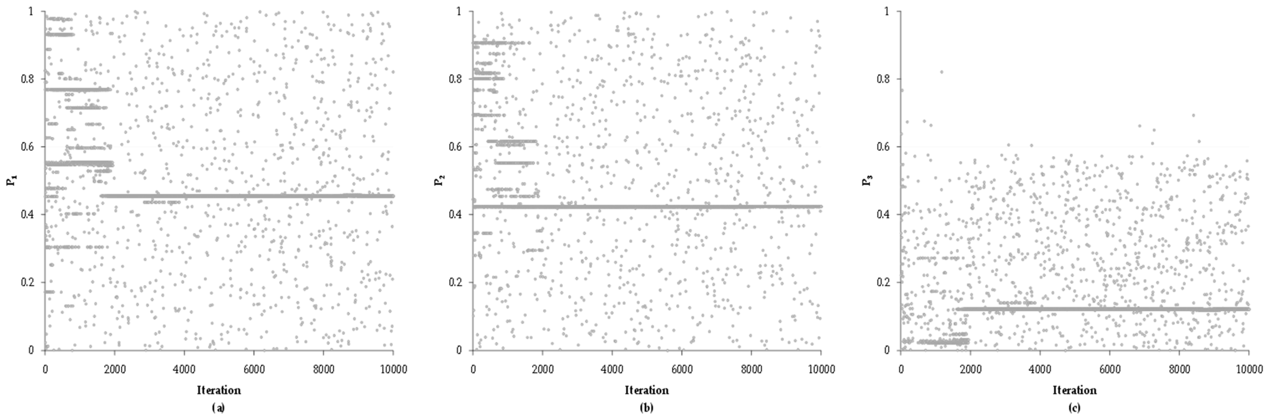
The final solution of station 10040 is shown below by graphing the stochastic optimization process for each of the parameters that constitute the EV1-3P function (Figure 4, Figure 5, Figure 6, Figure 7 and Figure 8).

The graphs associated with the stochastic process of optimization for each of the parameters in the EV1-3P function for station 10031 are shown in Figure 9, Figure 10, Figure 11, Figure 12 and Figure 13).

The optimized solution and the calculated value of the EEA to verify the goodness of the adjustment, carried out for both hydrometric stations, was recorded (

Table 5. Comparison of parameters obtained in the EV1-3P using Maximum Likelihood (ML) and harmonic search (HS) methods.

Parameter	10040		10031
	ML	HS	ML	HS
P1	0.34	0.62	0.10	0.45
ε1 (m3 s–1)	351.30	580.65	8.88	373.27
λ1 (m3 s–1)	254.99	510.30	7.97	206.95
P2	0.40	0.10	0.70	0.42
ε2 (m3 s–1)	898.68	3889.84	230.23	165.41
λ2 (m3 s–1)	121.96	1251.38	188.29	249.35
P3	0.26	0.28	0.20	0.12
ε3 (m3 s–1)	1893.20	882.79	999.90	1598.59
λ3 (m3 s–1)	1139.43	118.67	622.42	717.73
EEA	391	300.76	245	187.92

).

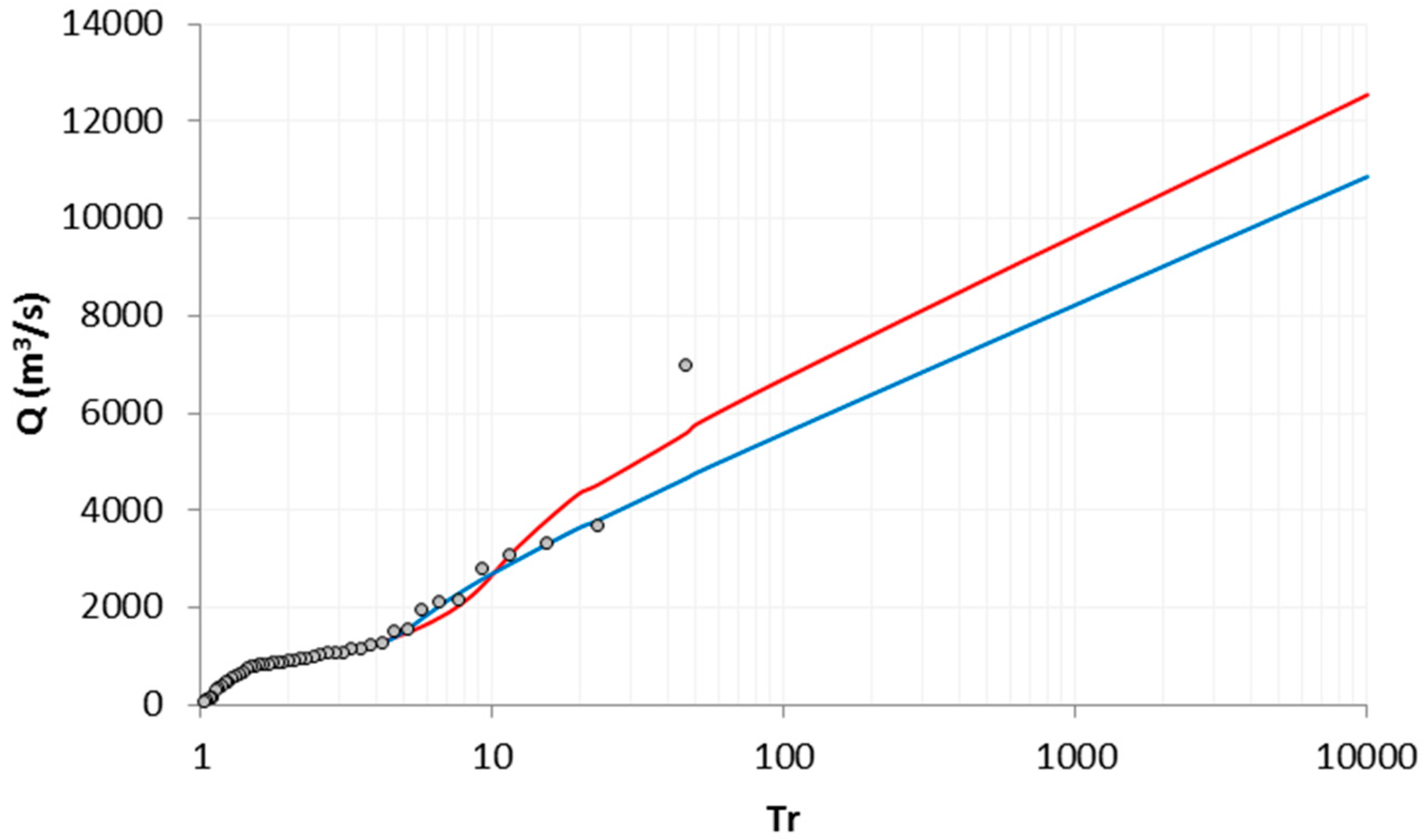
Using the optimized solution, design values were obtained for both stations for 20, 50, 100, 500, 1000, 5000, and 10000 years of return period (

Table 6. Comparison of the design values of gaging stations 10040 and 10031 obtained by using the parameters computed in the EV1-3P by using ML and HS methods.

Tr	QT (m3/s)
	10040		10031
	ML	HS	ML	HS
20	3652	4362	1778	2122
50	4770	5769	2401	2883
100	5583	6706	2849	3411
500	7435	8773	3863	4589
1000	8228	9647	4296	5089
5000	10068	11667	5299	6247
10000	10862	12545	5731	6745

). These values are used for the design of different engineering works and in our particular case, hydraulic infrastructure for the incidence of tropical cyclones, considering the level of confidence associated with their safety.

With the parameters computed in the EV1-3P by using ML and HS methods, the design value behavior for different return periods was calculated for both stations. Figure 14 and Figure 15 show the fitting with respect to the historical Q series.

4. Discussion

For the optimization of both stations, the parameter vectors xU and xL were defined according to the historical Q register. In the case of xL, taking care that it had to maintain physical sense for all the parameters of Equation (9), they adopted the value of zero, which corresponds to the absence of flow in the hydrometric station and to a null probability for the first and second population. xU is the value of the maximum annual flows of the sample and P is the probabilities of the first and second population. The calculation of P with the proposed HS meta-heuristic technique for the EV1-3P, from the multiple populations that compose the historical data sample, represents a great advantage over other procedures. Yue et al. [52] reports that the calculation of the probability parameter is sensitive to the correlation coefficient for defining the size of the populations, especially when the bivariate extreme-value distribution model with Gumbel marginals is used. This is not the case with HS, as all parameters are optimized simultaneously. It is important to emphasize that P₃, which represents the probability of the third population, is a function of P₁ and P₂ by means of the term (1 − (P₁ + P₂)), which indicates whether the data sample is adjusted to an EV1-3P function or should be adjusted to an EV1-2P function. It is important to mention that when processing samples from two populations, finding the P parameter is easier. Simply select the size of one of the series and the second will be defined [46,51].

The rest of the parameters were defined, and once the iterative processes of both hydrometric stations were initiated, the existence of convergence to the minimum possible value of the objective function could be appreciated (Figure 4 and Figure 9).

In the first case study, station 10040 provided 45 data points for which 4500 iterations were necessary before starting a gradual decrease in the EEA. Before that, we can observe a decrease with seasonality from 0.13 to 0.55 in the first 200 iterations. There was a then staggered decrease from 0.55 to 0.22 over 2500 iterations. In this case, the number of iterations is much higher than that reported in the literature for this sample size [20,38].

The mean of the 40 harmonic vectors with which harmonic memory was initiated corresponds to the same number of stochastic proposed initial solutions. The new model iterations replace the most unfavorable solution.

An important decrease in the average is observed in the first 1000 iterations, which indicates the speed of the method to converge on a solution. After that, the speed of convergence is reduced until iteration 6000, from which we can observe that practically, the solution that optimizes the eight parameters of the EV1-3P function has been reached.

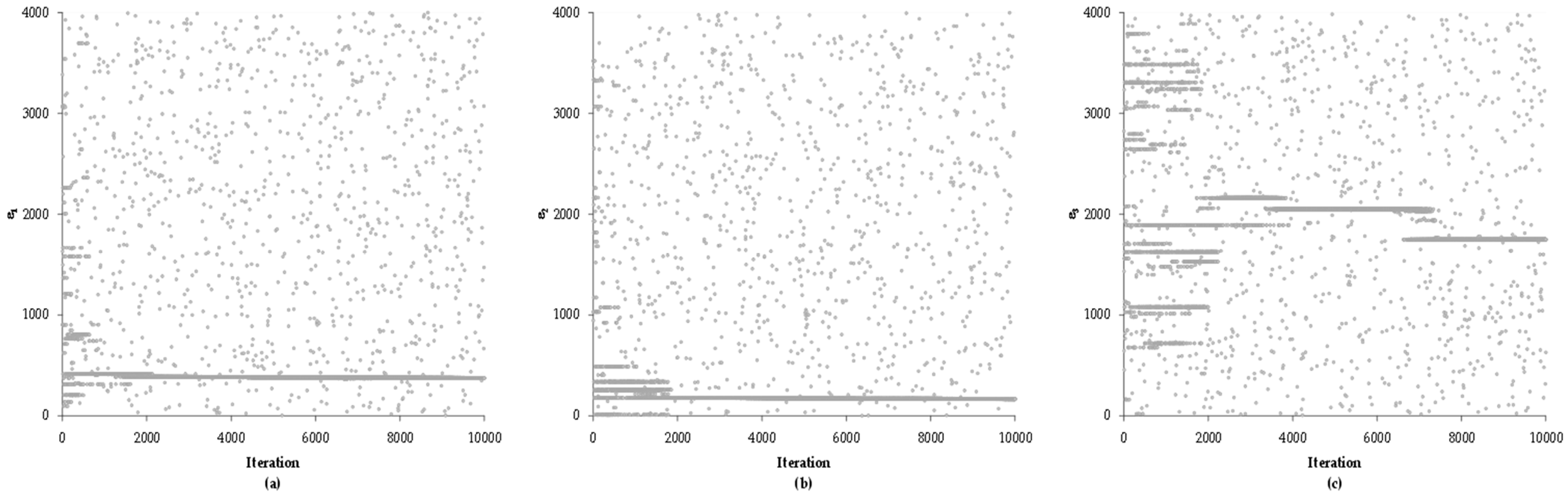
Figure 6, Figure 7 and Figure 8 represent the stochastic processes of probabilities, location, and scale parameters in the three populations of Equation (9). Overall P₂, ε₁, ε₃, λ₁, and λ₃ show significant variation in the first 2000 iterations, after which they begin to show asymptotic horizontal behaviors.

ε₂ and λ₂, contrary to P₂, require 6000 iterations prior to establishing the horizontal trend of solution, which suggests that the probability of the second population has a transcendental role in the optimization process. The results of this model are obtained with a faster convergence (less iterations) than the one reported in models in Sinsuphan et al. [30] and Yoon et al. [38].

These graphical behaviors are given by the successive repetition of the magnitude of each parameter with respect to the iterations performed. However, due to the generation of random numbers within the code, values are recorded that break the trend in a punctual manner, returning to count again in iterations after the horizontal trend.

In the second case study, 37 data points were considered from station 10031, which generated a much higher value of the EEA target function, starting with a magnitude of 0.95 (Figure 9) as opposed to 0.13 in the first case study (Figure 4).

At the beginning of the optimization process, minimal iterations were required to reduce the EEA value to 0.41. The number of iterations was reduced to 2000 and finally, this is the value of the final solution. This behavior reaffirms the efficiency of the meta-heuristic technique for minimizing the objective function (Equation (14)).

Similarly, the behavior shown by the average of the 40 vectors that constitute the harmonic memory starts with a value of 2.50 (Figure 10), as opposed to 0.45 in the first case study (Figure 5), which is derived from the lower dispersion shown by the data when plotted with respect to the reduced variable.

Nevertheless, there is an initial reduction in the average value until it reaches 1.25 in the first iterations, from which the slope of the curve is reduced, starting a less accelerated process until reaching a value of 0.30 in iteration 1000, presenting a slight seasonality. At 2000 iterations, the solution has been reached.

When graphing the successive behavior of the stochastic values of the probability in the three populations, variation can be observed in the first 2000 iterations to later establish the trend of solution.

Unlike the first case study, a greater stability is shown in P₁ and P₂, which therefore generates an associated stability in P₃ and specifically reduces the amplitude in its search interval, which is not greater than 0.60 in most cases.

Regarding the location parameters, it can be observed that both ε₁ and ε₂ experience trends in the first 2000 iterations, and the horizontal trend of solution resulting from the consecutive repetition of the response value is subsequently established. However, trends in small values are reflected in trends of significant magnitude in ε₃, which causes it to be established up to iteration 7000.

Finally, the location parameters λ₁ and λ₂ also presented several initial horizontal tendencies in the first 2000 iterations and later establish the solution tendency. However, defining λ₃ by means of the stochastic search showed an important oscillation even when it tends to reduce gradually without showing a solution tendency as marked as in the previous parameters.

With the eight parameters defined for the EV1-3P function in each of the stations, the maximum flows were calculated to compare them one by one with respect to the Q recorded and define the value of the EEA (Equation (14)).

When comparing the adjustment made using the ML technique carried out [16], a decrease of 90.24 units in the EEA is observed for hydrometric station 10040 and 57.08 units for hydrometric station 10031 (see Table 5). In the first case, there is a reduction of 23.07% in the reported values, and 23.29% in the second case, using a classical optimization technique with respect to the meta-heuristic technique used in this work.

When recording the information (Table 5) of both case studies for P₁, an increase in value is observed. In P₂ there is a decrease, while for P₃ there is little change. As P₁ increases, the values of ε and λ increase. In the case of P₃, its behavior is complementary with respect to ε and λ, with an important difference when associated with the reduced number of data points of the sample used.

In the graphical representation of the optimization carried out (Figure 14 and Figure 15), using the HS, the three flows of greater magnitude of the reduced variable calculated are greater than the historical ones registered, which allows the maximum flow of the calculated series to be closer in magnitude to the maximum flow registered. This is significantly reflected in the EEA value for the sample.

In the behavior described by the design values for higher return period magnitudes in both stations (Figure 15), suggest that the results estimated using the HS method produce an overestimate of approximately 20% in the design values for return periods greater than 10 years. For shorter return periods, in both methods there are no discrepancies between the design values.

In the optimization process, it is advisable to consider the largest possible series of maximum annual flow to improve the estimation in design values with a high return period.

In future works, the application of the EV1-3P to the rest of the stations in the state of Sinaloa will be explored to verify that the results obtained in this work can be generalized. If possible, this generalization process will study stations in other states of Mexico and other parts of the world that have the same effect of cyclonic events. Escalante-Sandoval [53] suggests that it is very important to consider the Mixed Weibull distribution and its bivariate option when analyzing floods generated by a mixture of two populations. In Latin America and the Caribbean, measurement continues to be one of the fragile points of modern hydrology. In addition to the problem of insufficient information, the traditional analysis of the frequency flows for extreme values implies the verification of the homogeneity of historical series. The fact that a historical series of data consists of several populations may be the result of a number of factors, including seasonal variations in flood occurrence mechanisms, e.g., hurricanes or the El Niño/La Niña phenomenon. The estimation of floods for a certain return period can be inefficient for design purposes. For this reason, the use of mixed distributions is a good option to improve the prediction of extreme floods. Extreme phenomena affecting Mexico, such as the occurrence of two hurricanes at the same time (Ingrid and Manuel in 2013), should be studied with mixed probability distributions of two or more populations [53]. Recent studies have shown that when using mixed distributions, such as Mixed Gumbel, Gumbel-Logistic and Gumbel-Hougaard Copula, the main problem is the adaptation of extreme values [54].

5. Conclusion

Having implemented an HS meta-heuristic technique for the EV1-3P of Q, it is concluded that it is an effective and efficient option for the simultaneous determination of the three location, the three scale, and the three probability parameters, according to the structure of nine parameters that conform to the structure of the function.

Likewise, it is established that it represents a better option for the analysis of frequency distribution in samples containing cyclonic and non-cyclonic events compared to classical techniques such as ML.

The decrease in the value of the EEA establishes that a better Q forecast is made depending on different return periods, with which the uncertainty of the design flows is reduced in regions periodically affected by cyclonic events, particularly in the coastal regions of the Pacific Ocean.

The mathematical tool presented here applies to runoff data. Therefore, future hydrological responses will have to be studied with the analysis of extreme events, as the processes of the hydrological cycle are sensitive to climate change. However, the proposed methodology can be used with other meteorological factors that have an influence on the runoff process, as extreme meteorological elements will impact in the calculation of runoff [55].