The Impact of the Two-Way Coupling between Wind Wave and Atmospheric Models on the Lower Atmosphere over the North Sea

Abstract

The effects of coupling between the atmospheric model of the Consortium for Small-Scale Modelling-Climate Limited-area Modelling (CCLM) and the wind wave model (WAM) on the lower atmosphere within the North Sea area are studied. Due to the two-way coupling between the models, the influences of wind waves and the atmosphere on each other can be determined. This two-way coupling between these models is enabled through the introduction of wave-induced drag into CCLM and updated winds into WAM. As a result of wave-induced drag, different atmospheric parameters are either directly or indirectly influenced by the wave conditions. The largest differences between the coupled and reference model simulation are found during storm events as well as in areas of steep gradients in the mean sea level pressure, wind speed or temperature. In the two-way coupled simulation, the position and strength of these gradients vary, compared to the reference simulation, leading to differences that spread throughout the entire planetary boundary layer and outside the coupled model area, thereby influencing the atmosphere over land and ocean, although not coupled to the wave model. Ultimately, the results of both model simulations are assessed against in situ and satellite measurements, with a better general performance of the two-way coupled simulation with respect to the observations.

1. Introduction

Wind induced waves at the surface of the ocean are well known to affect the overlying atmosphere. In 1989, Janssen [1] investigated the wave-induced stress and airflow drag over sea waves. Three years later, Janssen reported experimental evidence of the effects of surface waves on the airflow [2]. Since then, coupled atmosphere–wave models have been utilised in many studies to analyse the effects of wind waves on the atmosphere and vice versa. These studies addressed mainly the effects of coupling on idealised cyclones [3,4], hurricanes [5], wind waves [6], atmospheric [7] and wave forecasts [6] and climate [7].

The flow of air within the free atmosphere is determined by the balance between the pressure gradient and the Coriolis force. Closer to the surface, friction also plays a major role in the momentum balance. This friction leads to a cross-isobar flow. As a result, low-pressure systems fill more quickly [8]. Over the ocean, this friction is dependent on the sea state. In particular, young sea states are associated with rough airflow and high friction [8,9]. Hence, the largest changes in the surface roughness and friction velocity occur in areas of young sea states [10]. Consequently, this increased friction leads to more direct airflow into the centre of the low-pressure system, and thus the system fills up more quickly. On the other hand, enhanced friction leads to enhanced heat fluxes, which tend to deepen low-pressure systems [8]. Therefore, the effects wind waves have on the evolution of a low-pressure system are determined by the dominant processes through which the system develops. Momentum fluxes play a major role in the development of extratropical lows. Where an atmospheric model is coupled to a wave model, the momentum flux affected by wind waves causes less deepening of the lows during the model simulation [3,4,7,8]. For hurricanes, however, the temperature difference between the ocean and the atmosphere can become quite large. In this case, the heat flux can also play a major role in the development of the low. Bao et al. [5] demonstrated that a hurricane can become deeper due to the coupling between the atmospheric model and the wave model. Furthermore, feedbacks between wind waves and the atmosphere create nonlinear interactions within the dynamic structure of a storm or cyclone [10]. Katsafados et al. [10] also found that the planetary boundary layer (PBL) is thicker and more turbulent due to atmosphere–wave coupling. The impact of coupling on a single depression is also dependent on the model resolution. If the resolution is too coarse to resolve the processes involved, the effect caused by coupling the wave model to the atmospheric model vanishes [7,8,11]. Wu et al. [11] also analysed the effects of different roughness length parametrisations on the predictability of a storm, but none of the tested parametrisations could reproduce the results of the coupled model simulation.

The two-way coupling of wave and atmospheric models was introduced into the operational forecasts of the European Centre for Medium-Range Weather Forecasts (ECMWF) in 1998. This led to substantial improvements in various surface parameters, such as the 10 m wind speed and the significant wave height, and had modest impacts on the 1000 hPa and 500 hPa geopotential heights [7,8].

This two-way coupling also affects the climate across the troposphere. Janssen and Viterbo [12] and Janssen et al. [7] found significant impacts in the storm track area in both hemispheres, although the effect is more pronounced in the Southern Hemisphere. This discrepancy was attributed to the larger water surfaces surrounding the Antarctic continent and the less precise forecasts for the Southern Ocean due to the lack of observational data there [12]. These findings show that the effects of local wind waves produce teleconnections in the large-scale atmospheric system. Furthermore, the wind wave climate itself is affected by the coupling of wave and atmospheric models [13]. Weisse et al. 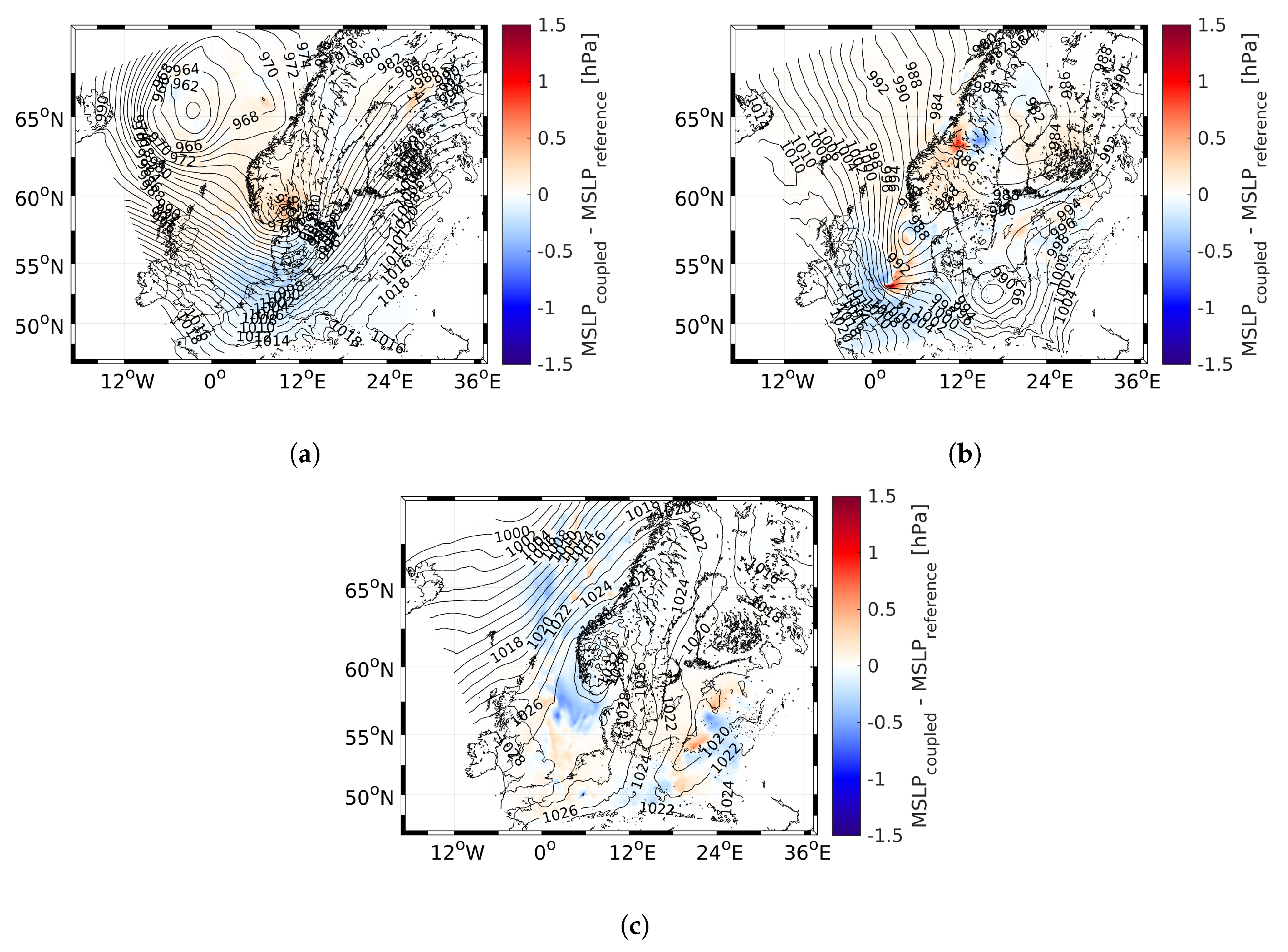[14] and Weisse and Schneggenburger [15] investigated the sensitivity of a regional atmospheric model to sea-state dependent roughness regarding the mean sea level pressure in the region of the North Atlantic Ocean. They, on the other hand, found no significant impact on the mean sea level pressure, when introducing wave-depended roughness to the atmospheric model.

The above mentioned studies focused on the impacts of the coupling between atmospheric and wave models close to the surface, whereas they paid little attention to differences that occur above the surface layer. Therefore, the present study further investigates under which conditions the coupling lead to differences in the atmospheric parameters within and at the height of the atmospheric boundary layer. The models and measurement data used for the analysis are described in the next section (Section 2). This is followed by an analysis of the general differences between the reference simulation and the coupled model simulation regarding the roughness length, 10 m wind speed and significant wave height (Section 3). In Section 4, an event with large changes close to the boundary layer height is identified and analysed in more detail. This is followed by a discussion of the results (Section 5). Finally, a summary and the conclusions of this analyses are given in Section 6.

2. Numerical Models, Model Set-Up and Measurement Data

2.1. Numerical Models

2.1.1. Atmospheric Model CCLM

This study employs the atmospheric model known as Consortium for Small-Scale Modelling (COSMO)-Climate Limited-area Modelling (CLM) Community (CCLM) version 4.8 [16], a non-hydrostatic regional climate model developed and applied by the CLM Community [17] on the basis of the numerical weather prediction model COSMO [18]. CCLM is based on the primitive equations that describe compressible flow in a moist atmosphere and uses the primitive momentum equations. The continuity equation is replaced by a prognostic equation for pressure perturbations from a reference state, which represents a time-independent dry atmosphere at rest. This atmosphere is prescribed as being horizontally homogeneous, vertically stratified and in hydrostatic balance.

The model domain of CCLM covers Northern Europe with a spatial resolution of 0.1${}^{\circ }$. In the vertical direction, 40 grid levels are used. The initial and boundary conditions are taken from 6-hourly ECMWF Re-analysis (ERA)-Interim analysis data [19,20].

2.1.2. Wave Model WAM

Here, the wind wave model (WAM) Cycle 4.5.4 is used [6,21,22]. In this version, depth refraction and wave breaking are taken into account. Consequently, this model set-up is suitable for shallow water applications. The directional resolution of the model is 15${}^{\circ }$. The model uses 30 frequencies logarithmically spaced from 0.04 to 0.66 Hz. The model domain covers the North Sea and has a spatial resolution of approximately 5 km (Figure 1). The values at the open boundaries of the model domain are taken from the European WAM (EWAM), the regional model of the Deutscher Wetterdienst (DWD).

2.1.3. Coupling between CCLM and WAM

The OASIS3-MCT version 2.0 coupler is used to couple the CCLM and WAM [6]. The fields that are exchanged in this study are the wind components as well as the roughness length. In the one-way coupled model simulation (hereafter called the reference model simulation), WAM receives the wind components from CCLM, and CCLM uses the Charnock parametrisation to calculate the roughness length over water surfaces [18]. In the two-way coupled model simulation (hereafter known as the coupled model simulation), WAM still receives the wind components from CCLM and additionally sends the roughness length calculated directly from the wind wave field back to CCLM. In order to determine the effects of the coupling of the wind wave model and the atmospheric model, the results of the two model simulations are compared. This is illustrated through the differences between the model simulations (reference and coupled) close to the surface but also in higher parts of the atmosphere.

2.2. Measurement Data

To determine whether the two-way coupling improves the model results, the simulations are compared with observational data. For this purpose, in situ measurements within the North Sea from the Global Telecommunication System (GTS) and satellite measurements from Sentinel-3A are chosen. The two data sets are described in the following sections.

2.2.1. In Situ Measurements

Most of the in situ measurement data of the significant wave height and wind speed used in this study are from the GTS. The data are obtained from and archived at the ECMWF [23]. Alternatively, the data are gathered by the ECMWF as part of the Joint Technical Commission for Oceanography and Marine Meteorology (JCOMM) wave forecast verification project [24]. The data are recorded either by moored wave data buoys, anchored at fixed locations to serve national forecasting needs, or by instruments mounted on platforms or rigs of the oil and gas industry. These data have been kindly provided to the meteorological community. As in [25], the wave height measurements are collocated with the model data using the closest grid point to the location of the in situ measurement and the wind speed measurements are interpolated to a height of 10 m above the surface and then collocated with the model using the closest grid point to the location of the observation. The locations of the in situ measurements are depicted in Figure 2.

2.2.2. Satellite Data

The significant wave height and wind speed observations from the Sentinel-3A satellite are used to compare the model results with satellite measurements. Sentinel-3A, which was launched in February 2016, is the first satellite that operates entirely in synthetic aperture radar (SAR) mode [26]. The revisit time of Sentinel-3A is 27 days. The data acquired by Sentinel-3A are retrieved from 1D profiles along the ground track of the satellite. The footprint size is between 1.5 and 10 km depending on the sea state across the track. The along-track resolution of Sentinel-3A is approximately 7 km for 1 Hz measurements. Figure 2 shows the locations of the satellite measurements. Because the quality of the data from Sentinel-3A is better than that of data from other satellites, especially close to the coast, the data from this satellite are chosen for comparisons with the model results [25]. The satellite data are collocated according to the nearest model grid point and the closest time with a maximum time lag of 30 min.

3. General Impacts of the Wave–Atmosphere Coupling

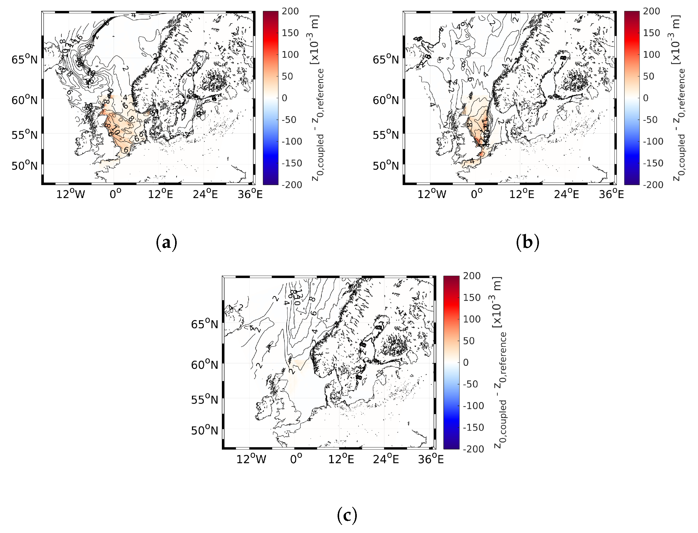
In the coupled model simulation, the roughness length calculated by WAM is passed to CCLM to ensure a roughness length over the ocean that is more precise than the parametrised roughness length used within the reference model simulation. Figure 3 shows the dependency of the roughness length on the wind speed (Figure 3a) and the friction velocity (Figure 3b). Clearly, the roughness length in the reference model simulation is underestimated compared with that in the coupled model simulation. In particular, at wind speeds exceeding 10 m s${}^{-1}$, the roughness length of the wave model becomes substantially larger than the parametrised roughness length. Additionally, the least-squares best-fit lines through the roughness lengths of the coupled model simulation show that the parametrised roughness length in CCLM is too small, especially at high wind speeds. The colour of the roughness lengths of WAM in Figure 3 indicates the corresponding wave age. These results illustrate that a young sea state creates a large surface roughness, as was also found by Janssen et al. [7], Janssen [8] and Katsafados et al. [10]. For wind speeds below approximately 15 m s${}^{-1}$, the largest roughness lengths are due to swell with large wave ages. However, this effect cannot be captured by parametrisations in the stand-alone atmospheric model [27]. The roughness length for areas covered by sea ice is set to 0.001 by CCLM, as shown by the black lines in Figure 3.

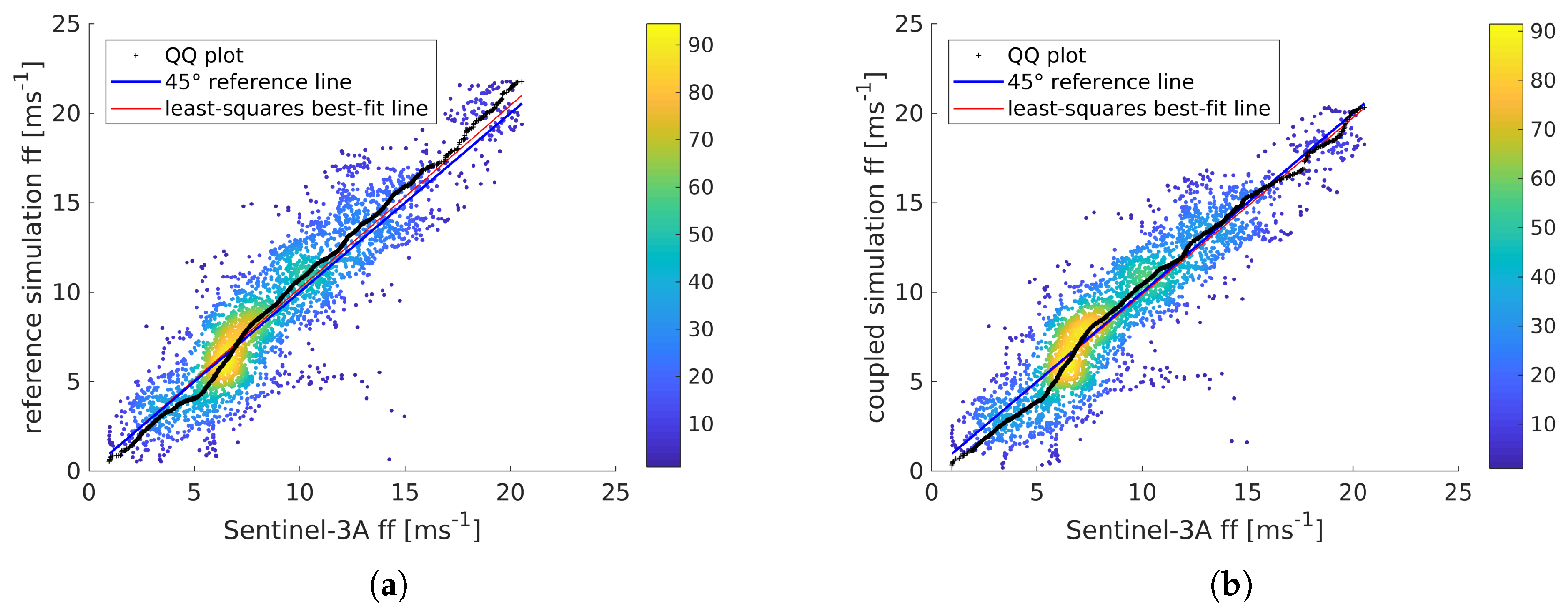
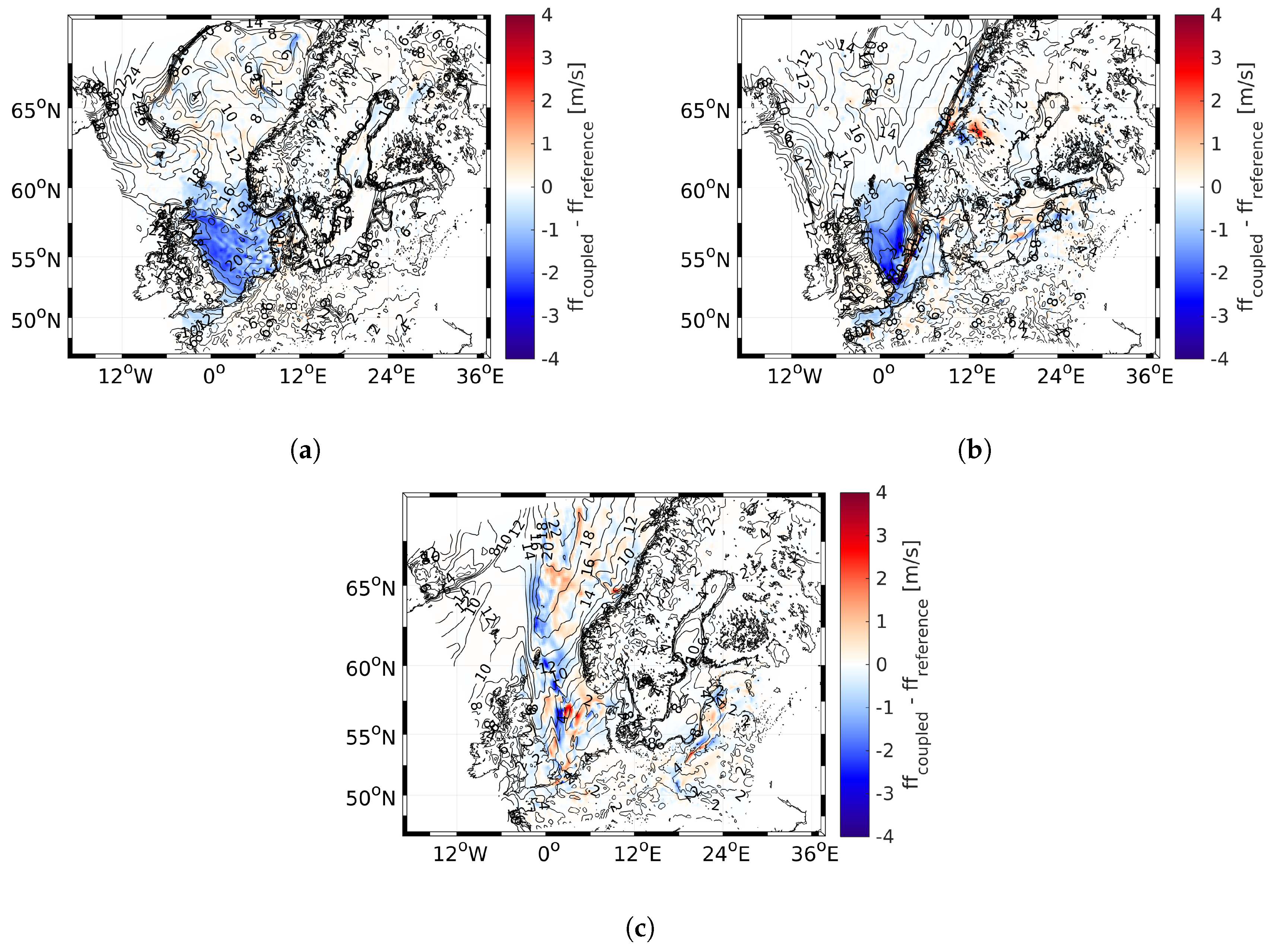
The wind speed and significant wave height are the most obvious parameters influenced by the coupling between the atmospheric model and wind wave model, since the wind is exchanged between the models and directly influences the significant wave height and, the other way round, the wave height directly influences the roughness length given back to the atmospheric model. Hence, the general influences of the two-way coupling on the wind speed and significant wave height are investigated. In Figure 4, the wind speeds modelled with both the reference model simulation (Figure 4a) and the coupled model simulation (Figure 4b) are compared with the wind speeds measured by the Sentinel-3A satellite. The reference model overestimates the wind speeds exceeding approximately 7 m s${}^{-1}$ (Figure 4a). Below 7 m s${}^{-1}$, CCLM underestimates the Sentinel-3A wind speeds. In the coupled model simulation, the overestimation of wind speed above approximately 7 m s${}^{-1}$ is reduced compared to the reference simulation. Furthermore, for high wind speeds (exceeding 15 m s${}^{-1}$), the overestimation is eliminated entirely (Figure 4b). However, at wind speeds below 7 m s${}^{-1}$, the coupled model simulation tends to produce a slightly larger underestimation than the reference model simulation. According to the statistical values calculated between the measured and modelled wind speeds, the results of the coupled model simulations are closer to the measurements than the results of the reference model simulation (

Table 1. Statistical values of the comparison between the wind speeds (ff) and significant wave heights (hs) measured by Sentinel-3A and the modelled wind speeds and significant wave heights.

	ff		hs
	Reference	Coupled	Reference	Coupled
Entries	3286		3284
Mean (Sentinel-3A)	8.85 m s${}^{-1}$		2.28 m
Mean (Model)	9.05 m s${}^{-1}$	8.77 m s${}^{-1}$	2.25 m	2.14 m
Standard Deviation (Sentinel-3A)	3.82 m s${}^{-1}$		1.38 m
Standard Deviation (Model)	4.35 m s${}^{-1}$	4.13 m s${}^{-1}$	1.49 m	1.35 m
Root Mean Square Error	1.94 m s${}^{-1}$	1.81 m s${}^{-1}$	0.49 m	0.45 m
Scatter Index	0.218	0.204	0.213	0.188
Bias	0.199 m s${}^{-1}$	−0.082 m s${}^{-1}$	−0.029 m	−0.136 m
Correlation	0.896	0.899	0.945	0.951

).

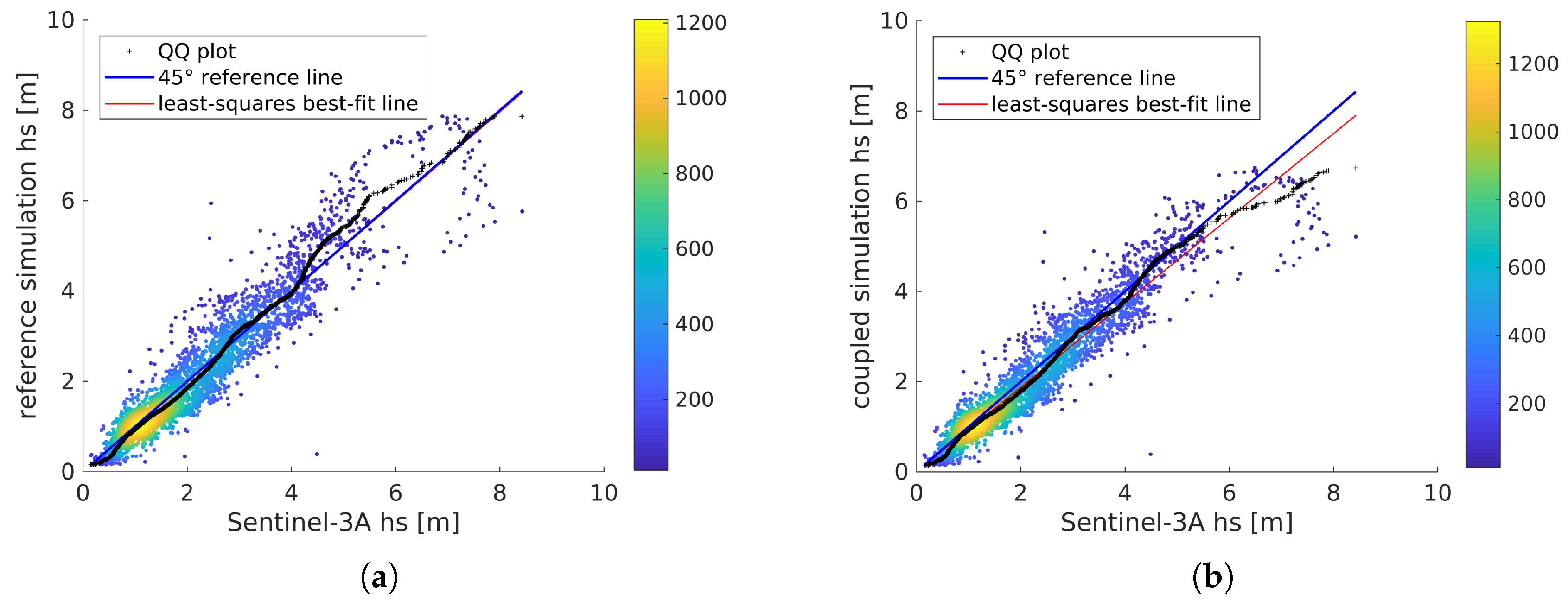
In the coupled model simulation, the significant wave height is influenced by changes in the wind speed, resulting in nonlinear feedback in both the atmospheric model and the wave model. The modelled significant wave heights below 4 m in both model simulations are in good agreement with the satellite measurements (Figure 5). In contrast, significant wave heights between 4 m and 7 m are overestimated by the reference model simulation, whereas larger significant wave heights are represented quite well by the reference model (Figure 5a). In the coupled model simulation, the significant wave height is depicted very well until the significant wave height reaches 6 m, while larger significant wave heights tend to be underestimated by the coupled model simulation relative to the satellite measurements during January 2017 (Figure 5b). Regarding the root mean square error, the scatter index and the correlation, the statistical parameters are improved for the coupled model simulation compared with those for the reference model simulation (Table 1).

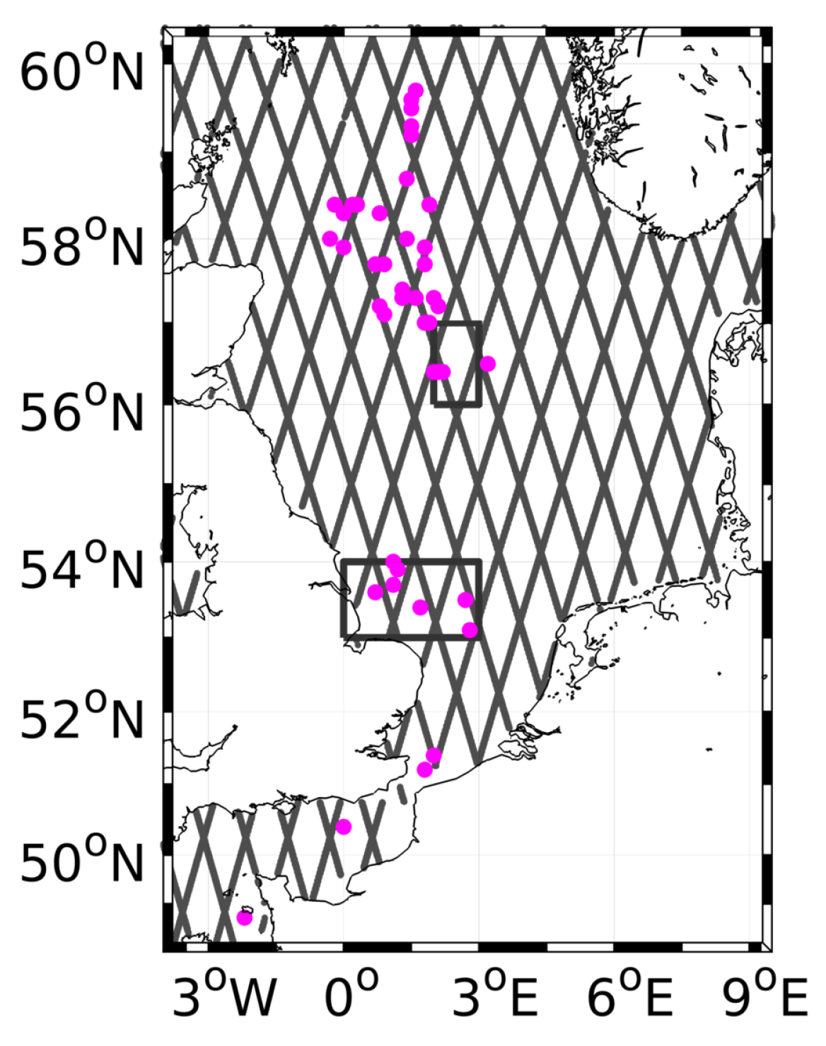
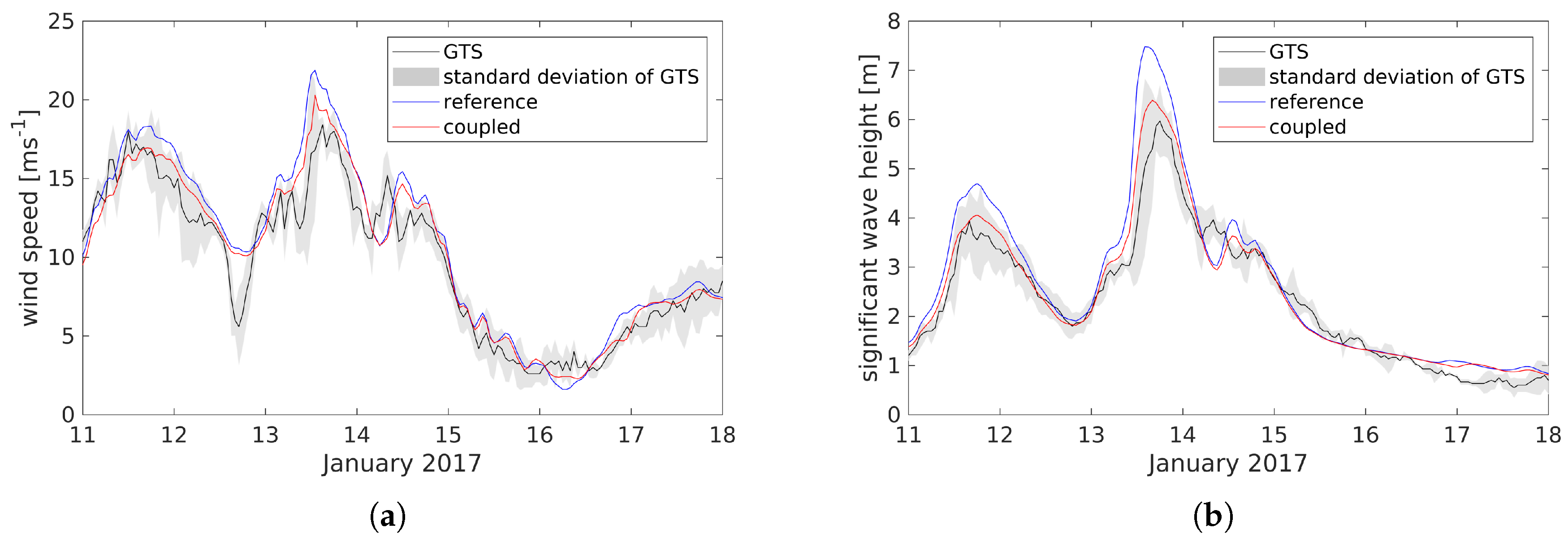
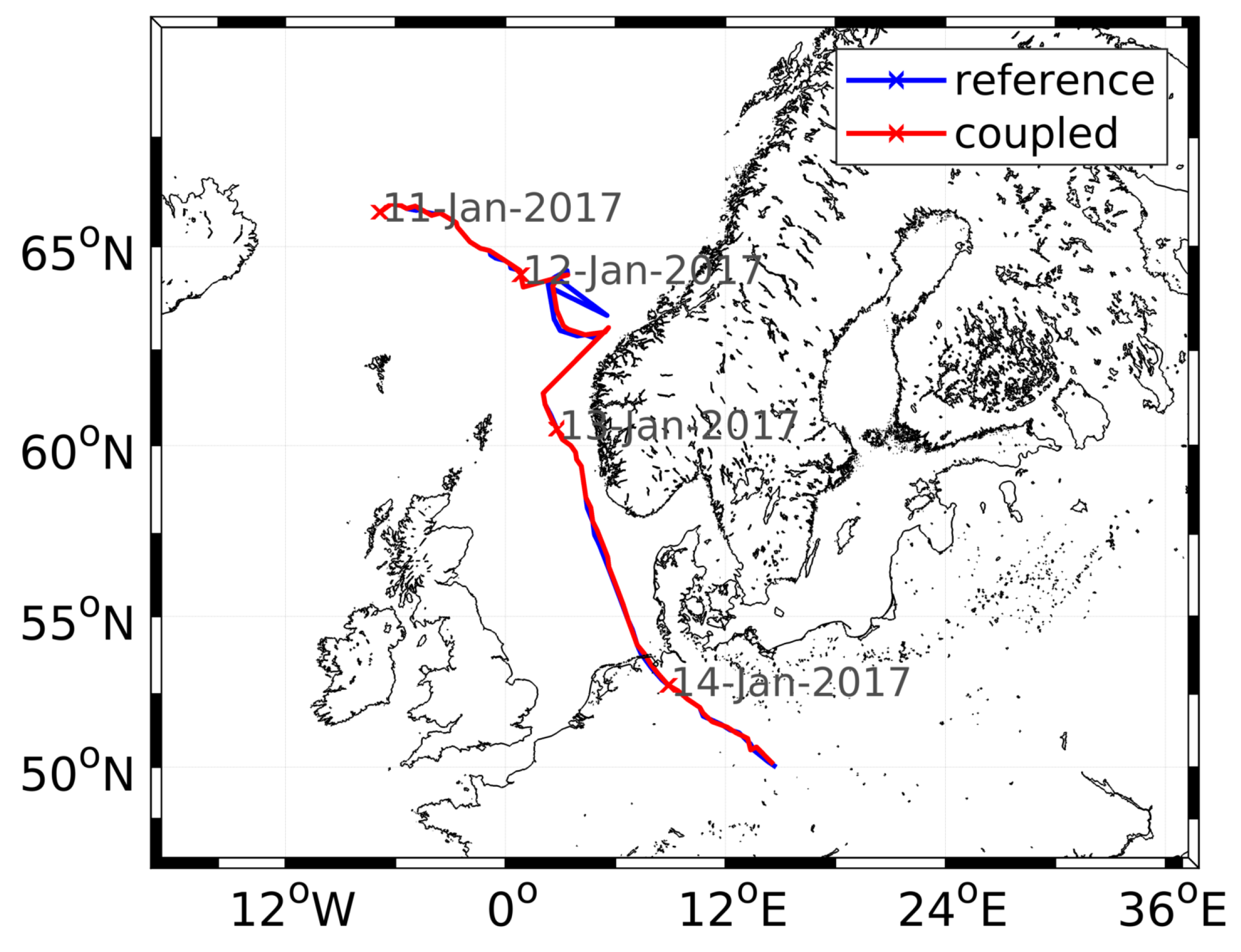
The largest differences both in the wind speed and in the significant wave height occur during extreme events with large wind speeds and significant wave heights (Figure 4 and Figure 5). Therefore, the model results are compared with GTS measurements recorded during one extreme event in January 2017 by buoys located off the coast of England (53${}^{\circ }$ N, 0${}^{\circ }$ E to 54${}^{\circ }$ N, 3${}^{\circ }$ E). For this comparison, the measurements acquired at the same time from the seven buoys within that small area (see the black box in Figure 2) are averaged. The results of the models collocated with the buoys are then averaged as well. As shown in Figure 6, the results of the coupled model simulation are closer to the observations than are the results of the reference model simulation. In particular, under the high wind speeds and large significant wave heights observed on the 11th/12th and 13th/14th of January 2017, the coupled model performs substantially better than the reference model. During these periods, the results of the reference model simulation are outside the standard deviation range of the GTS measurements, while the results of the coupled model simulation are well within the range of standard deviations. During the calm conditions after the storm, both model simulations produce rather similar results that are close to the measurements (Figure 6).

These findings illustrate that the overall agreement between the coupled model simulation and the observational data are better than the agreement between the reference model simulation and the observational data. This result is especially valid during extreme events. During calm conditions, the results of both model simulations are quite similar. The discrepancies in these model performances result from the underestimation of the roughness lengths by the CCLM parametrisation compared to the roughness lengths calculated by WAM. This underestimation is larger at higher wind speeds, which causes larger differences for extreme events.

4. Impact of the Two-Way Coupling of the Models on Processes within the PBL and Higher Layers of the Atmosphere

4.1. Temporal Variability within the PBL

Hovmöller diagrams are generated to determine the events corresponding to large effects within the PBL due to the coupling between CCLM and WAM. Figure 7 presents the Hovmöller diagrams for an area of 1${}^{\circ }$ by 1${}^{\circ }$ in the middle of the North Sea (symmetric around the point 56.5${}^{\circ }$ N, 2.5${}^{\circ }$ E, Figure 2) for January 2017. On 16 January 2017, an event can be observed that is associated with large differences in the pressure, temperature and wind speed close to the PBL height. A second event can be observed on 24 January 2017 with a recognizable temperature change. Both events are associated with quickly rising temperatures along warm fronts (Figure 7e). Additionally, during these events, the wind speed is relatively low (Figure 7c), and the surface pressure exceeds 1010 hPa (Figure 7a). To analyse these changes close to the PBL height, the time period between 11 January and the event on 16 January 2017 is investigated in more detail because the largest changes in all three parameters occur during this period. Additionally, on 13 January 2017, an event emerges that is characterised by pressure changes throughout the atmosphere.

4.2. Synoptic Situation

First, the synoptic situation during the time period from 11 to 16 January 2017 is discussed using the mean sea level pressure (MSLP) results from the reference model simulation. On 11 January 2017, the centre of the low-pressure system is located between Iceland and Norway, and a secondary low-pressure system is located over the southern coast of Norway close to Oslo (Figure 8a). The associated pressure gradient across the North Sea is quite steep, causing high northwesterly winds in the North Sea area. The secondary low moves northeastwards with increasing pressure in the centre and eventually vanishes over Norway. The main low-pressure system moves towards the coast of Norway, after which it moves south along the coast and crosses the North Sea with a convergence zone evolving from the centre to the British coast (Figure 8b). During this storm period, the wind speeds and significant wave heights are quite large. On 13 January 2017 at 9:00 p.m. UTC, the centre of the low-pressure system hits the East Frisian Islands along the German coast, after which it moves further southeastwards and fills up. After this low-pressure system moves out of the area, a high-pressure system develops over the North Sea (Figure 8c) in association with low wind speeds and low significant wave heights throughout that area.

4.3. Tracks of the Low-Pressure System

Next, the tracks of the low-pressure system in the reference and coupled model simulations are compared (Figure 9). The track of the low-pressure system is defined as the path of the minimum MSLP with time. The tracks in both model simulations are quite similar. The largest difference occurs when the system approaches the Norwegian coast. The core of the system is quite large, which makes the definition of the centre inaccurate. Nevertheless, the structure of the low-pressure system is very similar in both cases. The tracks in the reference and coupled model simulations of the low-pressure system across the North Sea before hitting the German coast are also very similar. Therefore, the two-way coupling between the wind wave model and the atmospheric model does not influence the track of this low-pressure system. One possible reason for this might be that the coupled area in this set-up is too small, with the low pressure system moving across that area quite fast. Therefore, the time the low pressure system has to adjust to the changed roughness length might be too short to develop a different track, as this was found by other studies [7].

4.4. Impact on the Roughness Length

The parameter within the atmospheric model that is directly changed by the coupling with the wind wave model is the roughness length. In the coupled model simulation, the roughness length is calculated in the wind wave model and then passed to the atmospheric model, whereas in the reference model simulation, the roughness length is calculated using the Charnock parametrisation [18].

On 11 January 2017 at 12:00 p.m. UTC, the roughness length in the coupled model simulation is enhanced compared to that in the reference model simulation (Figure 10a). When the low-pressure system moves across the North Sea, the roughness lengths are also enhanced west of the convergence zone (Figure 10b). These enhancements are associated with high wind speeds and large significant wave heights. On 16 January 2017 at 6:00 a.m. UTC, when the high-pressure system is located over the North Sea, these differences in the roughness length vanish (Figure 10c).

4.5. Impact on the Mean Sea Level Pressure

The differences in the roughness length discussed in the previous section (Section 4.4) lead to differences in the MSLP because the roughness length determines the direction of airflow into the low-pressure system [8]. Due to the enhanced surface roughness on 11 January 2017 at 12:00 p.m. UTC (Figure 10a), the airflow moves more directly into the low-pressure system, allowing the low-pressure system to fill up faster. Therefore, the pressure increases in the centre of the low-pressure system and decreases around the outside, letting the gradient across the North Sea decrease (Figure 11a).

Two days later, the largest changes in the MSLP can be found in the area of the convergence zone (Figure 11b) because the exact position of the convergence zone varies between the reference and coupled model simulations. This convergence zone moves farther to the east in the coupled model simulation. This effect can also be seen in the Hovmöller diagrams (Figure 7). At this time, a steep increase in the pressure can be detected throughout the entire atmosphere (Figure 7a). Because the convergence zone enters the investigated area earlier in the coupled model simulation, due to the shift towards the east, the pressure is increased throughout the entire atmosphere in the coupled model simulation (Figure 7b). On 16 January 2017 at 6:00 a.m. UTC, the high-pressure system is located over the North Sea.

4.6. Impact on the 10 m Wind Speed

On 11 January 2017 at 12:00 p.m. UTC, the wind speed is also reduced due to the two-way coupling between the atmosphere and the wind waves (Figure 12a). This is mainly due to the enhanced surface roughness (Figure 10a) of the ocean surface because enhanced friction reduces the wind speed close to the surface. In addition, the reduced pressure gradient (Figure 11a) contributes to a reduced wind speed within the North Sea area. Two days later, the largest impacts on the wind speed are observed along the convergence zone (Figure 12b). Slightly east of the convergence zone, the wind speed is enhanced. This corresponds to the shift of the convergence zone towards the east, as seen in the MSLP (Figure 11b). West of the convergence zone, where high wind speeds occur, the wind speed is again reduced due to the enhanced surface roughness. Due to the small pressure gradient across the North Sea on 16 January 2017 at 6:00 a.m. UTC (Figure 8c), the wind speed is considerably low (Figure 12c).

4.7. Impact on the Significant Wave Height

The significant wave height is reduced on 11 January 2017 at 12:00 p.m. UTC (Figure 13a). This reduction is due to the wind speed being reduced (Figure 12a), as the wind speed is passed from the atmospheric model to the wind wave model and therefore directly influences the significant wave height. This reduction reaches up to 1.4 m. The same can be seen two days later, when the significant wave height is reduced by up to 2.3 m west of the convergence zone, where significant wave heights reaching 10.5 m occur. On 16 January 2017 at 6:00 a.m. UTC, these changes in the significant wave height vanish, as the significant wave height is quite small during that time (Figure 13c) due to low wind speeds.

4.8. Impact on the Temperature at the 850 hPa Geopotential Height

On 16 January 2017 at 6:00 a.m. UTC, a warm front is located across the North Sea, which can be clearly seen in the map of the temperature at the 850 hPa geopotential height (Figure 14). The position and strength of this front differs between the coupled and reference model simulations. This explains the changes close to the PBL height seen in the Hovmöller diagrams (Figure 7). These changes also extend outside the coupled model area.

5. Discussion

In this study, we depicted the differences between single run experiments of one-way and two-way coupled model simulations, showing that the differences between coupled and reference simulation can still be detected at the height of the PBL for the event studied. One approach to test the significance of the findings is using ensemble simulations. The significance of the role of sea state dependent roughness for the performance of coupled wave-atmospheric models has been differently estimated in several previous publications [12,14]. The opinions range widely. Janssen and Viterbo [12] reported a significant impact of the sea-state dependent momentum exchange in their ensemble mean of a global model using 15 ensemble members and a horizontal resolution of 30 km. Furthermore, they showed that the effects of waves are propagating up to the higher levels in the atmosphere. On the contrary, Weisse et al. [14] and Weisse and Schneggenburger [15], who analysed the sea level pressure over the North Atlantic, claimed that the effects of wind waves in the coupled model are weaker than the natural variability and can not easily be discerned. In their analysis they used an ensemble of six members with a horizontal resolution of 0.5${}^{\circ }$, but did not analyse the propagation of signals in the atmospheric boundary layer and above.

Although the ensemble approach proved useful to compare the significance of effects resulting from using new parametrisation against the natural variability, there are a number of studies which do not use this approach [10,11]. Our study is one such example. We use a much finer resolution with the aim to illustrate situations under which the sea-state dependent momentum transfer would lead to substantial effects in both models. Our conclusions of the importance of sea state depended momentum exchange, in order to come closer to observational data, are more in line with these of Janssen and Viterbo [12], which might be due to the fact that our model resolution (0.1${}^{\circ }$) is closer to the one of Janssen and Viterbo [12] (30 km) than to the one of Weisse et al. [14] (0.5${}^{\circ }$). Knowing that the natural variability is strongly dependent on some other processes, which we did not address here, we will mention below some important issues first to address. One of these is to improve the model formulation of the atmospheric boundary layer. Another problem, when addressing the sea state dependent momentum exchange, would be to consider the coupled system of currents, waves and atmosphere. When addressing these issues in further studies, a deeper analysis with using model ensembles will be presented. Since the coupled model area in this study is rather small, the dependency of the changes found in this study on the size of the model domain, as well as different boundary conditions or different parametrisations of the roughness length, would be of interest.

6. Summary and Conclusions

In this study, the effects of coupling between an atmospheric model and a wind wave model, especially those on the PBL, are analysed. This coupling is enabled through the introduction of wave-induced drag in the atmospheric model and updated winds in the wind wave model.

The general performance of the coupled model system is better compared to the reference simulations with respect to observational data. The improvements in the coupled model system occur especially during extreme events because the influence of the enhanced surface roughness due to the coupling being largest at high wind speeds. During conditions of low wind speeds, both simulations are quite similar because the surface roughnesses calculated by WAM do not differ substantially from the surface roughnesses calculated by the parametrisation provided in CCLM.

Through the analysis of one event that affects the entire PBL, it becomes clear that the reference and coupled model simulation differ, especially along steep gradients, such as convergence zones and fronts. These differences are still present, when the significant wave height is already very small, and, therefore, the roughness length and variations in the roughness length are very small either. The differences between the reference and coupled simulation further extend outside the coupled model area over land and over uncoupled water surfaces.

This study demonstrates that the coupling between an atmospheric model and a wind wave model is necessary to obtain model results of wind speed and significant wave height closer to observational data with a better estimation of the roughness lengths over the oceans, also accounting for different wave conditions at similar wind speeds, following the conclusions from Janssen and Viterbo [12], Janssen et al. [7] and Wu et al. [11].