Towards Unifying the Planetary Boundary Layer and Shallow Convection in CAM5 with the Eddy-Diffusivity/Mass-Flux Approach

Abstract

The modular structure of the boundary layer and convection parameterizations in atmospheric models have long been affecting the numerical representation of subgrid-scale motions and their mutual interactions. A promising alternative, the eddy-diffusivity/mass-flux approach (EDMF), has the potential for unifying the existing formulations into a consistent scheme and improving some of the long-standing issues. This study documents a step towards developing such a unified approach by implementing a stochastic multi-plume EDMF scheme into the Community Atmosphere Model (Version 5.0). Its performance in single-column mode is evaluated against the control parameterization and large-eddy simulation (LES) for two benchmark cases: marine and continental shallow convection. Overall, the results for the two parameterizations agree well with each other and with LES in terms of mean profiles of moist conserved variables and their vertical fluxes, as well as the updraft properties. However, systematic differences between the two schemes, especially for transient continental convection, are also documented. Using EDMF helps improve some of the parameterized features of shallow convection. In particular, for the highest tested vertical resolution, the EDMF cloud base and top heights and the vertical fluxes of energy and water are remarkably close to LES.

1. Introduction

A fundamental difficulty in the coarse-resolution modeling of atmospheric subgrid-scale transport by weather and climate models is to optimize the complexity of its parameterizations: it should be high enough to facilitate a realistic representation of large-scale turbulence effects, yet low enough to limit their impact on available computational power. As different types of atmospheric motions exhibit different dominant features, they can be differently parameterized. Consequently, general circulation models (GCMs) tend to split them into several generic regimes: planetary boundary layer, shallow convection, and deep convection.

This modularity is also present in the Community Atmosphere Model (CAM; in this paper, we use the 5.0 version of CAM, also referred to as CAM5), which serves as a testbed for the current study. Merging all the regimes/modules together requires formulating criteria for their activations (i.e., trigger functions) and for their harmonic interactions (e.g., closure techniques). Additional complexity comes with cloud microphysics, which has to be properly handled by these schemes. An important drawback to modular parameterizations is that representing different types of convection within a grid box, or smooth and continuous transitions between different regimes, can be significantly impeded [1,2].

Historically, the development of convection parameterizations was largely motivated by the hot-tower hypothesis [3] proposed to explain the transport of moist static energy into the upper troposphere. Since then, different approaches have been proposed (for a review, see [4]), with the most popular one based on the mass-flux concept [5,6,7]. For this approach, the non-local vertical transport is solely controlled by the well-organized convective structures. The planetary boundary layer parameterizations, on the other hand, are commonly represented using the eddy-diffusivity approach.

In this paper, we use a unified approach to modeling subgrid transport in GCMs, the eddy-diffusivity/mass-flux (EDMF) parameterization [8,9,10,11,12,13], which has the potential to reduce the modularity and complexity of the parameterization algorithms significantly. Its main advantage is the ability to represent simultaneously boundary layer turbulence and different types of convection within a grid box, as modeled by a spectrum of plumes developing in a turbulent environment, without any arbitrary separation among the regimes. As a result, it removes the need for using closure techniques to determine interactions between the modules representing different processes (e.g., cloud base closure for coupling the dry boundary layer and the moist convective layer aloft [14]). In addition, for the process-splitting models [15] (such as CAM), it helps avoid the problems associated with determining an order in which the parameterizations/modules need to be called.

It should be mentioned that other approaches have been proposed to date to unify the representation of boundary layer and convection in GCMs. For example, two different unified parameterizations have been implemented in CAM: UNICON [16] and CLUBB [17]. The UNICON scheme employs the mass-flux approach and unifies shallow and deep convection. The CLUBB scheme imposes double-Gaussian distributions to represent subgrid variability to unify the boundary layer and shallow convection. This particular scheme includes several additional prognostic equations for higher moments of the model variables, which increases the scheme’s complexity and computational cost.

In this work, the multi-plume EDMF scheme is implemented in the CAM’s computational framework by replacing the original shallow convection module and merging the new one with the turbulence module. It is further tested in a single column model (SCM) configuration for two shallow-convection cases: the Barbados Oceanographic and Meteorological Experiment (BOMEX) and the Atmospheric Radiation Measurement (ARM) Program, which represent, respectively, quasi-stationary (i.e., marine) and diurnal (i.e., continental) shallow convection. Results of the simulations are compared against the original set of CAM’s parameterizations, as well as large-eddy simulation (LES).

The paper is organized as follows: Section 2 describes key features of the implemented EDMF scheme. The setup of the experiments is given in Section 3, and the results are presented in Section 4 (for the BOMEX case) and Section 5 (for the ARM case). The summary and conclusions are provided in Section 6. Technical details on the implementation of the new scheme into CAM’s numerical framework are given in the Appendix A.

2. Stochastic Multi-Plume EDMF Scheme

In the multi-plume eddy-diffusivity/mass-flux approach, the vertical subgrid turbulent transport is split into the local (ED) and non-local (MF) contributions:

$$\overline{w^{\prime }{\psi }^{\prime }}=-K_{\psi }\frac{\partial \overline{\psi }}{\partial z}+\sum _{i=1}^I{a}_i{w}_i({\psi }_i-\overline{\psi }),$$

(1)

where $\psi$ is the transported quantity, w the vertical velocity, K the eddy-diffusivity/viscosity coefficient for the local transport, i the index of the ith updraft (and thus, $a_i$, $w_i$, and ${\psi }_i$ refer to the values for the ith updraft), I the total number of updrafts (here, I = 20, which is sufficient to minimize the sensitivity of the results to I, as shown in [18]), $a_i$ the updraft area, and primes denote deviations from the grid-mean values denoted with overbars. Below, we describe how the two components are parameterized.

2.1. Mass-Flux Parameterization

The mass-flux formulation follows [18], neglecting the non-local transport within the environment. The updrafts are rooted at the surface, regardless of the model’s resolution, and extend up to the level of vanishing vertical velocity. They can saturate and produce condensed water, with the associated latent heating contributing to the buoyancy (the implemented version does not allow for rain formation since the study only focuses on the dry and shallow convection). Their properties are controlled by two factors: surface conditions and lateral entrainment. Surface conditions determine the initial buoyancy and vertical velocity of an updraft and are sampled from the right tails of the prescribed joint-normal probability density functions (PDFs) of the temperature, water vapor mixing ratio, and vertical velocity. Therefore, the underlying assumption is that the updrafts are formed by the most buoyant/energetic portions of the near-surface air [19]. In the model, the plumes are assumed horizontally homogeneous and interact with the properties of grid-mean fields via entrainment and buoyancy [20].

Given the state of the atmosphere the updrafts/plumes are assumed to be fully-developed and stationary. This means that temporal development of the plumes is not explicitly represented, and their ensembles at different time steps are not correlated. In particular, the number of updrafts used to represent convection can also change in time. The updrafts are designed to transport moist-conserved thermodynamic variables (i.e., liquid water potential temperature ${\theta }_l$ and total water mixing ratio $q_t$), horizontal momentum, and optionally, other fields. Note that, in general, the two thermodynamic variables do not account for the precipitating water, which has to be treated separately due to sedimentation, yielding additional sources for ${\theta }_l$ and $q_t$ [18].

Based on the rising parcel model for cumulus towers [21], the updraft properties required in Equation (1) are obtained from a steady-state plume equation describing the behavior of a transported variable ${\psi }_i$ with height:

$$\frac{\partial {\psi }_i}{\partial z}={ϵ}_i(\overline{\psi }-{\psi }_i)+\frac{S_{\psi ,i}}{w_i},$$

(2)

where ${ϵ}_i$ is the entrainment rate profile for the ith updraft, the first term on the r.h.s. represents the dilution by lateral entrainment, while the second term combines all other sink/source terms for ${\psi }_i$ (e.g., precipitation for thermodynamic variables or pressure gradient force for horizontal momentum, as shown in [22]). To integrate this equation, one needs to know the associated vertical velocity profile $w_i$ and the boundary condition for ${\psi }_i$ at the surface.

The updraft vertical velocity equation can be obtained from Equation (2), using an additional parameterization of the pressure effects, and is given by (e.g., [11]):

$$\frac{1}{2}\frac{\partial w_i^2}{\partial z}=a{B}_i-b{ϵ}_i{w}_i^2,$$

(3)

where $a=1$ and $b=1.5$ (cf. [13,23]), $B_i$ is the plume’s buoyancy (i.e., the excess of its density temperature over the environmental value), and the last term is a combination of the entrainment and the form drag suppressing the vertical motion. As mentioned above, surface conditions needed for integrating Equation (3) come from the assumed PDF for w, while those for integrating Equation (2) are from the corresponding PDFs for moisture and temperature. The horizontal area of each updraft is for convenience assumed constant with height and defined by the relative area of the associated bin from the near-surface velocity distribution. Therefore, total surface updraft area is equivalent to the fractional area of the PDF used to initiate the plume ensemble. Changes in the total updraft area aloft depend on the number of plumes that survive up to a certain height. The fraction of the PDFs that is used to initiate the plumes is fixed at around 15%.

Following [24], lateral entrainment, which controls the rate of dilution of the transported quantities, is parameterized as a stochastic process. The vertical profile of the entrainment rate is given by a random sequence of discrete entrainment events, independently calculated for each plume. The number of entrainment events depends on the distance $\Delta z$ traveled by the plume and is given by:

$${ϵ}_i(\Delta z)=\frac{E_0}{\Delta z}\mathcal{P}\left(\frac{\Delta z}{L_0}\right),$$

(4)

where $E_0$ is the intensity of an entrainment event defined as a fraction of the plume mass flux, $L_0$ is the entrainment length, and $\mathcal{P}$ the Poisson distribution describing a random number of entrainment events occurring along the distance $\Delta z$. Here, $E_0$ is set to 0.15, and the entrainment length is a function of the cloud layer thickness (taken from the previous time step):

$$L_0=max\left(L_{00},a_0(z_t-z_b)\right),$$

(5)

where $L_{00}$ = 40 m, $a_0$ = 0.1, and $z_t$ and $z_b$ are the cloud top and bottom heights, respectively. This translates into smaller entrainment rates for deeper clouds [13,25,26]. We also tested a fixed value for $L_0$, as in other EDMF studies, although the results were less consistent with LES.

Variability among the plumes is ensured by using both different boundary conditions for integrating their properties in the vertical and stochastic entrainment [18]. The multi-plume approach does not require any additional closures that are rather common in other types of convection parameterizations (e.g., [5,6]). Moreover, since different types of convection can co-exist within a subgrid domain, there is no need for an arbitrary separation of atmospheric convection into shallow or dry convection (i.e., dry updrafts can continue rising as moist updrafts upon favorable conditions), as is the case for the default CAM configuration.

2.2. Eddy-Diffusivity Parameterization

A complementary part of the EDMF scheme is the eddy-diffusivity parameterization of the local transport outside of convective plumes. Of several different diagnostic eddy-diffusivity schemes available in CAM, we chose the Holstag-Boville-Rash (HBR) scheme, which is an extension of [27], as it performs best for the current model configuration. Note that in previous implementations of the multi-plume model [13,18], the ED part was based on the prognostic equation for turbulent kinetic energy, which is not the case for the selected scheme.

In the diagnostic HBR scheme, two regions are distinguished that are characterized by different exchange coefficients: free troposphere and boundary layer. The free-tropospheric coefficients for heat, moisture, and momentum are defined using a standard formulation based on the Richardson number:

$$K=l^{2}Sf\left(Ri\right),$$

(6)

where l is the mixing length, S denotes the magnitude of the vertical shear of horizontal wind, and $Ri$ is the gradient Richardson number:

$$Ri=\frac{g}{{\theta }_v}\frac{\partial {\theta }_v/\partial z}{S^2},$$

(7)

where g is the acceleration of gravity and ${\theta }_v$ denotes virtual potential temperature. The function of the Richardson number, which is different for scalars and momentum, follows [27].

For the boundary layer, the exchange coefficients are calculated using:

$$K=\kappa w_{t}z{\left(1-\frac{z}{H}\right)}^2,$$

(8)

where $\kappa$ is the von Karman constant, $w_t$ denotes a characteristic turbulent velocity scale (different for scalars and momentum), and H is the boundary layer height. The exact formulations of $w_t$ and H can also be found in [27]. The HBR scheme additionally modifies K at the boundary layer top into:

$$K=\frac{0.2\left(w_{*}^3+5u_{*}^3\right)}{B_{ge}},$$

(9)

where $w_{*}$ and $u_{*}$ are the vertical and horizontal velocity scales [28,29], and

$$B_{ge}=\frac{g}{{\theta }_v}\frac{\partial {\theta }_v}{\partial z}H$$

(10)

is called the buoyancy gradient enhancement. This correction helps provide a smoother transition for the mixing coefficients between the dry and moist layers, which in the original EDMF version is provided by a TKE closure modified to match LES results [18]. Note that the vertical profile of K within the boundary layer has a cubic shape with the maximum at around one third of the layer height. The default HBR scheme accounts for non-local transport via the counter-gradient term; however, this option is switched off to avoid double-counting since the counter-gradient transport is already represented by the mass-flux component.

3. Setup of the Experiments

3.1. Configuration Overview

The numerical experiments simulated in this study included two well-known benchmark studies: BOMEX [30] and ARM [31]. The BOMEX case represents shallow quasi-stationary non-precipitating convection over the ocean, while the ARM case is an example of continental convection driven by the diurnal cycle of surface fluxes. For each case, we ran three simulations using 30, 60, and 120 stretched vertical levels, with a 300-s time step. The chosen spatial and temporal resolutions were a subset of CAM’s standard values. Time integration for the BOMEX and ARM cases was 6 and 14.5 h, respectively. The precipitation formation was switched off since the analyzed cases are known to be virtually unaffected by this process. The CAM’s configuration remained unchanged for all the simulations, both for EDMF and the default convection scheme, the latter briefly described next.

3.2. Reference Models

As a reference, we used both the default CAM5 configuration and large-eddy simulations. The LES results for BOMEX were produced by an ensemble of models [30] and are widely used for the evaluation and basic calibration of convection parameterizations. Additionally, LES results for ARM were produced by the Jet Propulsion Laboratory LES model [32] following the setup described in [31].

The default CAM configuration employed the University of Washington shallow convection [33] and moist turbulence [33] parameterizations (SHUW hereafter), the latter diagnosing local mixing both in the subcloud and cloud layers. The SHUW scheme models convection as a bulk entraining-detraining plume. The plume was initialized at the cloud base with the help of a closure using the integrated turbulent kinetic energy in the boundary layer and convection inhibition integrated from the boundary layer top to the level of free convection. The entrainment and detrainment rates were calculated using a buoyancy-sorting algorithm. The scheme included the parameterization of penetrative entrainment in the overshooting zone. The updraft fraction area was not allowed to exceed 0.1, and the condensed cloud water within the core was limited by 1.5 g kg${}^{-1}$. The convective fluxes in the boundary layer were reconstructed using a cumulus ventilation procedure. The operational default CAM5 configuration that was used in this study employs a default set of parameters, and thus, its performance may be different from that shown in other studies (e.g., [34,35]).

4. Results: Steady-State Marine Convection

For the BOMEX case, we analyzed solutions averaged over the last three simulation hours as in [16]. The convective boundary layer, which includes the subcloud and cloud layers, was resolved in CAM with 9, 17, and 33 levels for the three applied resolutions (i.e., 30, 60, and 120 levels). The subcloud layer itself was resolved with 4, 7, and 13 levels, respectively. A quasi-steady solution was reached by a near-balance between turbulence, subsidence, and large-scale forcings of temperature and moisture.

4.1. Thermodynamic Profiles

Figure 1 shows the mean profiles of liquid water potential temperature and total water mixing ratio from the three models compared. The simulated profiles agreed well across the resolutions with only small differences between them regarding mostly the cloud layer. Specifically, SHUW tended to transport slightly more heat and moisture into the upper part of the cloud layer (extending between 500 m and 1800–1900 m), as was also documented in [16]. This led to a decreased amount of moisture and increased liquid water potential temperature below 1500 m. On the other hand, EDMF tended to provide slightly stronger transport in the subcloud layer with a larger accumulation of water near below 1500 m. For the higher vertical resolution simulations, the EDMF results were closer to LES.

4.2. Thermodynamic Subgrid Vertical Flux Profiles

The simulated consistency of the heat and moisture profiles (Figure 1) resulted from the consistent subgrid turbulent fluxes of these quantities (Figure 2; contributions from the mass-flux transport alone are also shown). The single-column model results mostly fell within the envelope of the LES ensemble defined as the range between the first and the third quartiles. Their bottom boundary values were determined by the prescribed surface fluxes, to which they smoothly converged.

In the subcloud layer, the transport was clearly dominated by local turbulence, which became practically negligible in the cloud layer. Note that the non-local part for SHUW was reconstructed below the cloud base (as explained in [33]), while for EDMF, it was explicitly represented by dry (i.e., unsaturated) updrafts that could saturate above. As a consequence, it linearly grew with height for SHUW regardless of the resolution. For EDMF, however, it grew with a height similar to SHUW only at the coarsest resolution, but remained relatively constant above the surface layer at the finest resolution. The relative contribution of the non-local part depended on the intensity of local turbulence and increased/decreased as the eddy-diffusivity coefficient was arbitrarily decreased/increased (not shown). This mechanism of self-adjustment made the EDMF results relatively robust to changes in the magnitude of the local term within the range of a few tens of percent. Similar results were previously reported by [36]. Note, however, that the robustness of the results regarded the intensity of local turbulence within the well-mixed layer, given a certain profile of the turbulent mixing coefficients. For different profiles, these interactions at the top of the boundary layer may be different depending on the strength of turbulent mixing in the conditionally unstable layer.

In the cloud layer, EDMF tended to simulate slightly larger fluxes of moisture and more negative fluxes of liquid water potential temperature below 1500 m. The relationship reversed above, leading to the observed differences in the mean profiles of moist-conserved variables from Figure 1. The vertical range of the parameterized convection tended to decrease for finer resolutions.

4.3. Updraft Properties

Since turbulent transport in the cloud layer was dominated by the mass flux associated with updrafts; here, we compare basic updraft properties to evaluate how this aspect of convection is represented by the two parameterizations. The reference LES models from [30] define the updrafts as grid points with positive buoyancy (with respect to the horizontal mean) that contain cloud water, which are considered to belong to cloud cores. Additionally, they also define cloud regions that do not need to be positively buoyant. Conditionally-sampled properties of these two types of air yielded the cloud-core means and the cloud means that were previously used to constrain the parameterized updraft properties [13,36,37].

Figure 3 compares the following updraft properties: updraft area, vertical velocity, liquid water mixing ratio, and the excess of the total water mixing ratio and liquid water potential temperature over the grid-mean values. For SHUW, the properties always describe a single bulk updraft, while for EDMF they represent the area-weighted average over the saturated updrafts that still exist at a given height.

Profiles of the updraft area between SHUW and EDMF differed most notably around the cloud base height (where the bulk updraft was initialized), as the former always reached 0.1 (i.e., the configurable maximum allowed by the scheme). The SHUW updraft area abruptly decreased aloft to follow the cloud-core means from LES in a similar fashion for the three applied resolutions. On the contrary, EDMF simulated much smaller cloud-base maxima falling between the cloud-core means and the cloud means from LES, with their values aloft remaining closer to the cloud mean profiles. It should be reminded that the fractional areas of individual updrafts in EDMF were fixed at the values prescribed at the surface from the right tail of the near-surface distribution of vertical velocity [18]. Since the total updraft area was defined as a sum of their fractional areas, it can only change if the number of saturated ensemble members changes with height (i.e., terminates or evaporates all condensed water).

The vertical velocity profiles showed that the smallest differences between EDMF and SHUW occurred around the cloud base, where the spread of LES values was also the smallest. The differences significantly amplified with height as the growth rate for EDMF was much lower than for SHUW. Consequently, the EDMF profiles followed the cloud means, for all three resolutions, while the SHUW profiles followed, or even slightly exceeded, the cloud-core means. Note that although the bulk updraft area for SHUW dropped to almost zero above 1500 m, the actual termination level was much higher, as indicated by the vertical range of the profiles. Although the upper part of the updraft was less important for the mass flux due to only a residual updraft area there, SHUW tended to develop deeper convective layers than EDMF and LES. Because the vertical mass-flux was a product of the updraft area and the velocity, the above-described differences between SHUW and EDMF largely canceled each other out, and the resulting mass flux was comparable for the two models (not shown).

The profiles of the liquid water mixing ratio were fairly similar to those for the vertical velocity. Mean values and the spread of the LES results were zero at the cloud base and gradually increased above it. Contrary to the vertical velocity, however, the cloud-core values and the cloud values both monotonically grew throughout the entire layer. This behavior was also captured by the single-column models, with the EDMF profiles being closer to the cloud values and the SHUW profiles closer to the cloud-core values. The SHUW profiles saturated at 1.5 g kg${}^{-1}$, as dictated by the configurable limit for that parameterization, with the excess of water detrained into the environment.

Finally, profiles of the excess of moist-conserved variables largely followed the LES results, which were characterized by a notably smaller spread than the distributions of vertical velocity and updraft liquid water mixing ratio. Interestingly, SHUW remained more consistent in terms of total water mixing ratio, while EDMF more closely followed LESs for liquid water potential temperature, with neither of the models representing all the analyzed features perfectly. Overall, however, EDMF tended to be closer to LES than SHUW, which may be important for coupling the scheme with microphysics that is sensitive to the details of updraft dynamics and thermodynamics.

5. Results: Diurnal Cycle of Continental Convection

For the ARM case, convection was forced by the surface fluxes of heat and moisture that became positive after 11:30 UTC (5:30 local time), peaked between 18:30 and 19:30 UTC (12:30–13:30 local time), and decreased in the local evening [31]. Due to the large changes in the forcings and the lack of a steady-state solution, the case was generally more challenging to simulate by single-column parameterizations [31,36], partly also due to changing interactions between the local and non-local turbulence.

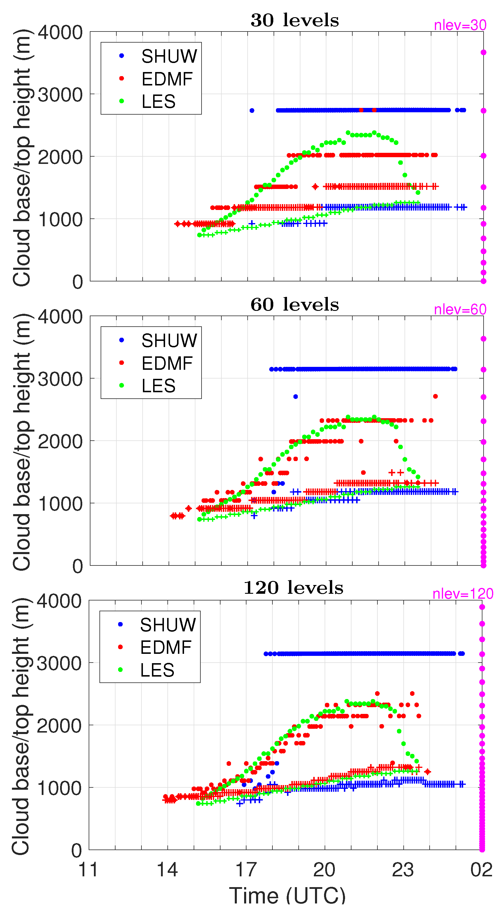
5.1. Convective Layer Evolution

Figure 4 shows time series of the cloud base and cloud top heights from SHUW, EDMF, and LES, for the three applied resolutions. Two significant differences between EDMF and SHUW were apparent: the timing of moist convection and its vertical extent. Other differences included a higher cloud base for EDMF in the last several hours (for the lowest resolution) and a stronger sensitivity of the EDMF results to changes in the resolution.

To understand these differences, one needs to look into the design of the two parameterizations. In the EDMF scheme, convective updrafts were formed when the surface buoyancy flux became positive (i.e., in the early morning). Convection started developing from dry updrafts that gradually deepened with time, and as soon as they reached the condensation level, shallow convection set in. On the contrary, SHUW used a trigger function based on convective inhibition to control the timing indirectly. These difference caused shallow convection to start roughly 1 h earlier (or 2 h later) for EDMF (for SHUW) than for LES. For the vertical extent, this metric was defined in EDMF as the height of the deepest moist updraft in the ensemble, while for SHUW was calculated as the level where the moist bulk plume terminated. Note, however, that the range of convective updrafts was less important for the vertical transport that primarily depended on the updraft area and vertical velocity, to be discussed later. A very promising result from the EDMF model was that, for the highest vertical resolutions, the EDMF results for cloud base/top height were remarkably close to the LES results. Their evolution was also smoother with time.

5.2. Thermodynamic Profiles

In Figure 5 and Figure 6, mean profiles of the total water mixing ratio and liquid water potential temperature are shown at four UTC times: 14:30, 17:30, 20:30, and 23:30 (i.e., 8:30, 11:30, 14:30, and 17:30 local time), as in [31]. Each profile represents an hourly mean (i.e., ±0.5 h) to reduce its temporal variability. Given the increased complexity of the problem, the two single-column models simulated the evolution of the profiles well, regardless of the resolution, although their discrepancy with respect to LES was now bigger than for BOMEX.

For the total water mixing ratio, moisture supply from the surface in the early simulation hours tended to be most quickly transported upwards by EDMF, with the weakest transport by LES. However, the ensemble LES results from ([31], Figure 4 therein) suggested that this transport should actually be more efficient at that time than in our LES.At later times, EDMF tended to transport more moisture from the subcloud layer into the cloud layer than SHUW did, but the efficiency of the transport in the upper part of cloud layer was stronger for SHUW. This led to the accumulation of moisture between 1100 and 1500 m for EDMF at 23:30 UTC, which was most apparent at the finest resolution. A cloud water deficiency of a similar magnitude between 1700 and 2200 m and a much larger accumulation above 2500 m occurred for SHUW. The accumulation of moisture simulated by EDMF right above the boundary layer strongly depended on the type of eddy-diffusivity parameterization used (not shown).

The behavior of the liquid water potential temperature profiles correlated well with that for the moisture profiles. For instance, the most intense vertical transport around 14:30 UTC was simulated by EDMF, resulting in the fastest deepening of the boundary layer at that time. Their final profiles (i.e., at 23:30 UTC) were slightly cooler than for LES in the regions of moisture excess (between 1100 m and 1500 m for EDMF and above 2500 m for SHUW) and warmer in the regions of moisture deficit (mostly for SHUW, between 1700 m and 2200 m). It should be stressed that the simulated differences between SHUW and EDMF for the thermodynamic fields were mostly within the spread of the LES ensemble results from [31]. Note that [31] compared the potential temperature rather than liquid water potential temperature, which generally resulted in a larger spread of the results due to the contribution from liquid water. However, this contribution strongly decreased around 23:30 UTC. Moreover, the spread in their LES ensemble results seemed comparable for both dry and moist parts of the convective layer, with the largest differences for the vertical extent of convection.

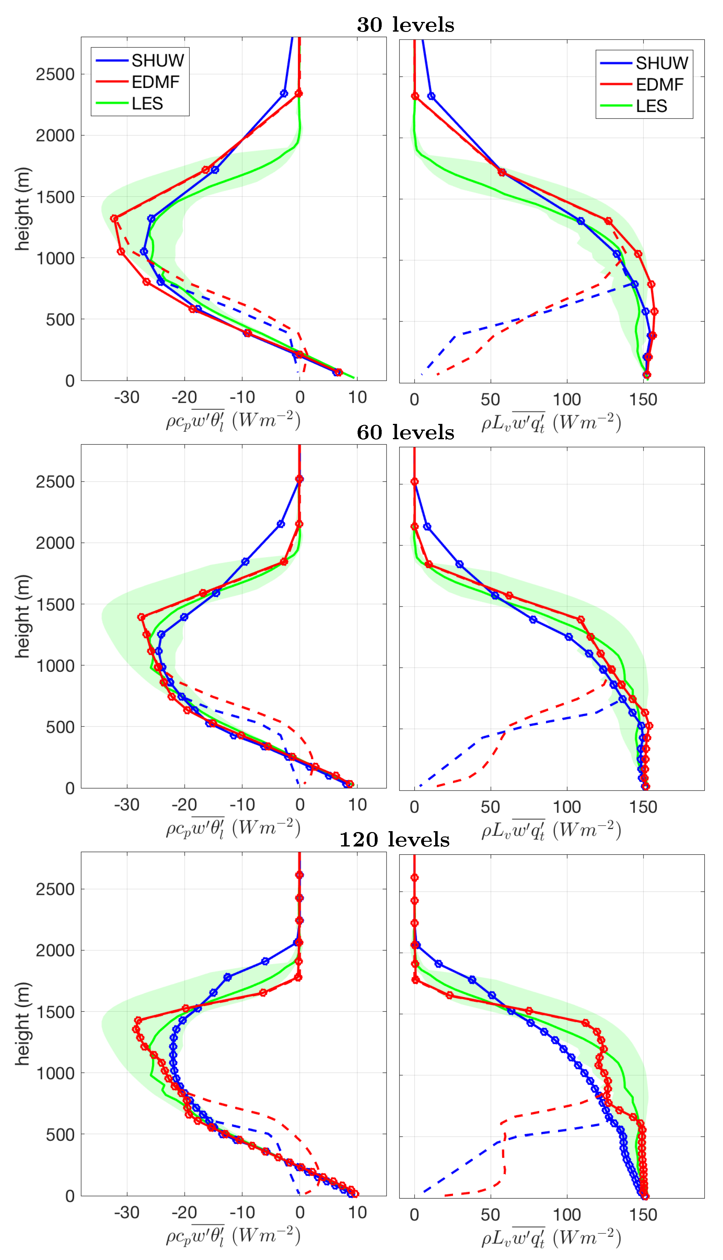
5.3. Parameterized Fluxes of Heat and Moisture

Mean profiles of the corresponding fluxes of moist-conserved variables are shown in Figure 7 and Figure 8. The spatial structure and the temporal changes of these fluxes provided an explanation of the simulated structure and changes of the mean profiles. As for the BOMEX case, bottom boundary conditions for the fluxes were prescribed, and the models smoothly converged to their changing-in-time values.

The morning profiles (i.e., at 14:30 UTC or 9:30 local time) were typical for the development of dry boundary layers. The fastest deepening of the layer for EDMF was the result of the largest entrainment flux at its top. At that time, the entire SHUW contribution to the temperature and moisture fluxes came from the local mixing, while for EDMF, it was already strongly affected by the dry mass-flux transport. The three models yielded more consistent results at 17:30 UTC, when the relative EDMF mass-flux contribution reduced and the local mixing intensified, while moist convection began to form in SHUW. At 20:30 UTC, both the SHUW and EDMF profiles still agreed well with LES; however, the former model decreased the mass-flux transport within the convective layer at the finest resolution. Note that the mass-flux contribution reached its maximum at higher levels for EDMF than for SHUW, but then dropped more rapidly with height, which is reflected in Figure 4 by a shallower cloud layer, especially at the coarsest resolution. When convective activity strongly deceased at 23:30 UTC, the magnitude of the EDMF convective transport in the subcloud and cloud layers became similar. On the contrary, SHUW tended to produce much larger convective fluxes in the upper part of the convective layer, especially at the finest resolution. The EDMF results were remarkably close to LES for the higher vertical resolutions at the time of peak convection (20:30 UTC). This was due to a sufficiently large number of levels within the cloud layer to represent the variability in the vertical range of the plumes.

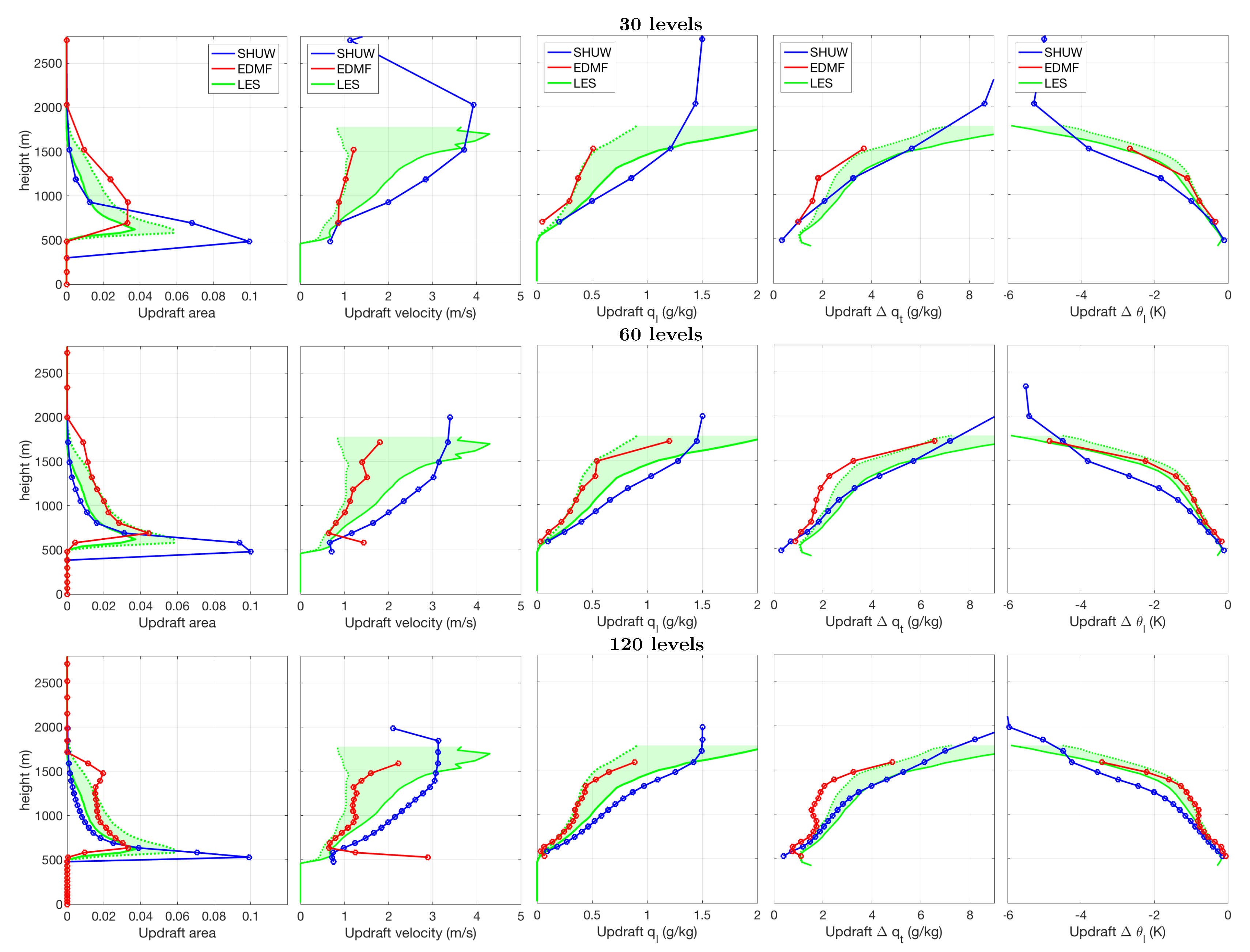
5.4. Updraft Properties

The comparison of the mean updraft properties (i.e., updraft area, vertical velocity, updraft liquid water mixing ratio, and the excess of the total water mixing ratio and liquid water potential temperature over the grid-mean values) between SHUW, EDMF, and LES for the three applied resolutions is shown in Figure 9 and Figure 10. The profiles represent hourly means around the times: 18:30 UTC and 20:30 UTC, similarly to [31].

The parameterized thermodynamic updraft properties largely followed the LES results and were robust to the applied changes in the resolution for both parameterizations. The largest differences regarded the mean dynamic properties: updraft area and vertical velocity, which was also documented for the BOMEX case. Again, the SHUW updraft areas started from much larger values around the cloud base, but more strongly decreased with height. Simultaneously, SHUW updraft velocity increased more strongly, exceeding the cloud-core LES values at most of the model levels. On the other hand, EDMF underestimated the updraft area near the cloud base, but vertical velocity was mostly in between the cloud-core and the cloud values from LES. The large vertical velocity at the lowest level of the cloud layer that occasionally appeared in the EDMF results was caused by strong and relatively moist updrafts that reached their saturation level lower than most of the ensemble members. This velocity decreased above when it was calculated over a larger ensemble (as seen by an increased updraft area). Liquid water for EDMF remained within the LES envelope defined by the cloud-core and the cloud values, while for SHUW, they were close, but mostly exceeded the LES maxima. Again, the cloud water limiters applied in SHUW did not allow the scheme to keep more than 1.5 gkg${}^{-1}$ in the bulk updraft, which was less important for the mass flux above roughly 2500 m where the updraft area was almost negligible.

The cloud layer at 18:30 UTC was generally shallower than at 20:30 UTC, and the main difference between these two times regarded reduced maximum updraft areas and stronger vertical velocities at the later time that were qualitatively represented by the two parameterizations. The documented differences between SHUW and EDMF in terms of the updraft properties seemed systematic as they had the same sign and a similar magnitude for the two simulated convective cases.

6. Summary and Conclusions

This study documented an important step towards developing a unified parameterization of subgrid atmospheric transport suitable for global circulation models. With the ultimate goal of replacing the modular structure of currently-used parameterizations with a consistent scheme, we tested the multi-plume eddy-diffusivity mass-flux (EDMF) parameterization that can simultaneously represent different types of turbulent transport within the subgrid domain, here limited to dry and moist shallow convection. The EDMF approach was devoid of arbitrary closures or trigger functions typically used to merge different parameterizations. The new scheme was implemented in the Community Atmosphere Model within the planetary boundary layer module. Hence, the original diffusion solver was adapted to calculate both the eddy-diffusivity and mass-flux contributions together. The single-column model version was used to simulate two shallow-convection cases: maritime (BOMEX) and continental (ARM) ones. The results of the simulations were compared against the default (modular) model configuration (SHUW), as well as large-eddy simulation (LES).

The results showed a good agreement of the implemented scheme both with the SHUW and LES models as documented by the comparison of the mean profiles of moist conserved variables and their vertical fluxes and the properties of moist updrafts: updraft area, vertical velocity, condensed water, and the excess of the total water mixing ratio and liquid water potential temperature over the grid-mean values. The simulated differences between SHUW and EDMF mostly remained within the envelope defined by the spread of LES results. The largest differences regarded much higher values of the total updraft area for SHUW than for EDMF near the cloud base that more strongly decreased with height. Correspondingly, the magnitude of vertical velocity for SHUW more strongly increased with height. In this respect, EDMF agreed better with LES, although it somewhat underestimated cloud cover around the cloud base.

One particularly interesting benefit of using the multi-plume EDMF parameterization was that it more realistically represented some aspects of convection such as the timing and the vertical extent of the cloud layer. Furthermore, contrary to the commonly-used approximation that the eddy-diffusivity term is entirely responsible for the fluxes in the subcloud layer, the conducted experiments indicated a notable contribution from the mass-flux term in that layer as well. The obtained results are encouraging since the formulation of the EDMF parameterization offered a more consistent approach to simulating atmospheric convection in a unified manner. Of note is the fact that the EDMF parameterization was remarkably close to the LES results, for the highest resolution, for the cloud base and top height evolution in the ARM case, and for the vertical temperature and water fluxes when convection was more intense.

Building on this experience, we plan to extend the evaluation of the model performance to include three-dimensional scenarios, after developing a microphysics scheme fully consistent with EDMF. Another important aspect worth exploring is the numerical performance of the scheme and its optimal coupling with the CAM’s framework. In the long term, the EDMF scheme is meant to include the deep convection parameterization, as discussed in [38,39], with a potential scale adaptivity for the mass-flux (cf. [40]) and eddy-diffusivity (cf. [41]) parts.

References

1. Guichard, F.; Petch, J.C.; Redelsperger, J.L.; Bechtold, P.; Chaboureau, J.P.; Cheinet, S.; Grabowski, W.; Grenier, H.; Jones, C.G.; Köhler, M.; et al. Modelling the diurnal cycle of deep precipitating convection over land with cloud-resolving models and single-column models. Q. J. R. Met. Soc. 2004, 130, 3139–3172. [Google Scholar] [CrossRef]
2. Teixeira, J.; Cardoso, S.; Bonazzola, M.; Cole, J.; DelGenio, A.; DeMott, C.; Franklin, C.; Hannay, C.; Jakob, C.; Jiao, Y.; et al. Tropical and Subtropical Cloud Transitions in Weather and Climate Prediction Models: The GCSS/WGNE Pacific Cross-Section Intercomparison (GPCI). J. Clim. 2011, 24, 5223–5256. [Google Scholar] [CrossRef] [Green Version]
3. Riehl, H.; Malkus, J.S. On the heat balance in the equatorial trough zone. Geophysica 1958, 6, 503–538. [Google Scholar]
4. Plant, R.S.; Yano, J.I. Parameterization of Atmospheric Convection; Imperial College Press: London, UK, 2015. [Google Scholar]
5. Arakawa, A.; Schubert, W.H. Interaction of a Cumulus Cloud Ensemble with the Large-Scale Environment, Part I. J. Atmos. Sci. 1974, 31, 674–701. [Google Scholar] [CrossRef] [Green Version]
6. Tiedtke, M. A Comprehensive Mass Flux Scheme for Cumulus Parameterization in Large-Scale Models. Mon. Weather Rev. 1989, 117, 1779–1800. [Google Scholar] [CrossRef] [Green Version]
7. Bechtold, P.; Bazile, E.; Guichard, F.; Mascart, P.; Richard, E. A mass-flux convection scheme for regional and global models. Q. J. R. Met. Soc. 2001, 127, 869–886. [Google Scholar] [CrossRef]
8. Siebesma, A.P.; Teixeira, J. An Advection–Diffusion Scheme for the Convective Boundary Layer: Description and 1D Results. In Proceedings of the American Meteorological Society 14th Symposium on Boundary Layer and Turbulence, Aspen, CO, USA, 7–11 August 2000; pp. 133–136. [Google Scholar]
9. Teixeira, J.; Siebesma, A. A Mass Flux/K-Diffusion Approach to the Parameterization of the Convective Boundary Layer: Global Model Results. In Proceedings of the American Meteorological Society 14th Symposium on Boundary Layers and Turbulence, Aspen, CO, USA, 7–11 August 2000; pp. 231–234. [Google Scholar]
10. Angevine, W.M. An Integrated Turbulence Scheme for Boundary Layers with Shallow Cumulus Applied to Pollutant Transport. J. Appl. Meteorol. 2005, 44, 1436–1452. [Google Scholar] [CrossRef]
11. Siebesma, P.A.; Soares, P.M.M.; Teixeira, J. A combined eddy-diffusivity mass-flux approach for the convective boundary layer. J. Atmos. Sci. 2007, 64, 1230–1248. [Google Scholar] [CrossRef]
12. Angevine, W.M. Performance of an Eddy Diffusivity–Mass Flux Scheme for Shallow Cumulus Boundary Layers. Mon. Weather Rev. 2010, 138, 2895–2912. [Google Scholar] [CrossRef]
13. Suselj, K.; Teixeira, J.; Chung, D. A Unified Model for Moist Convective Boundary Layers Based on a Stochastic Eddy-Diffusivity/Mass-Flux Parameterization. J. Atmos. Sci. 2013, 70, 1929–1953. [Google Scholar] [CrossRef]
14. Neggers, R.A.J.; Siebesma, A.P.; Lenderink, G.; Holtslag, A.A.M. An Evaluation of Mass Flux Closures for Diurnal Cycles of Shallow Cumulus. Mon. Weather Rev. 2004, 132, 2525–2538. [Google Scholar] [CrossRef] [Green Version]
15. Teixeira, J. Boundary Layer Clouds in Large Scale Atmospheric Models: Cloud Schemes and Numerical Aspects; ECMWF: Reading, UK, 2000; 190p. [Google Scholar]
16. Park, S. A Unified Convection Scheme (UNICON). Part II: Simulation. J. Atmos. Sci. 2014, 71, 3931–3973. [Google Scholar] [CrossRef]
17. Bogenschutz, P.A.; Gettelman, A.; Morrison, H.; Larson, V.E.; Craig, C.; Schanen, D.P. Higher-Order Turbulence Closure and Its Impact on Climate Simulations in the Community Atmosphere Model. J. Clim. 2013, 26, 9655–9676. [Google Scholar] [CrossRef]
18. Suselj, K.; Kurowski, M.J.; Teixeira, J. On the Factors Controlling the Development of Shallow Convection in Eddy-Diffusivity/Mass-Flux Models. J. Atmos. Sci. 2019, 76, 433–456. [Google Scholar] [CrossRef]
19. Cheinet, S. A Multiple Mass Flux Parameterization for the Surface-Generated Convection. Part II: Cloudy Cores. J. Atmos. Sci. 2004, 61, 1093–1113. [Google Scholar] [CrossRef]
20. Kurowski, M.J.; Suselj, K.; Grabowski, W.W. Is Shallow Convection Sensitive to Environmental Heterogeneities? Geophys. Res. Lett. 2019, 46, 1785–1793. [Google Scholar] [CrossRef]
21. Simpson, J.; Wiggert, V. Models of precipitating cumulus towers. Mon. Weather Rev. 1969, 97, 471–489. [Google Scholar] [CrossRef]
22. Romps, D. On the equivalence of two schemes for convective momentum transport. J. Atmos. Sci. 2012, 69, 3491–3500. [Google Scholar] [CrossRef]
23. De Roode, S.R.; Siebesma, A.P.; Jonker, H.J.J.; de Voogd, Y. Parameterization of the Vertical Velocity Equation for Shallow Cumulus Clouds. J. Atmos. Sci. 2012, 140, 2424–2436. [Google Scholar] [CrossRef] [Green Version]
24. Romps, D.M.; Kuang, Z. Nature versus Nurture in Shallow Convection. J. Atmos. Sci. 2010, 67, 1655–1666. [Google Scholar] [CrossRef] [Green Version]
25. Soares, P.M.M.; Miranda, P.M.A.; Siebesma, A.P.; Teixeira, J. An eddy-diffusivity/mass-flux parametrization for dry and shallow cumulus convection. Q. J. R. Meteorol. Soc. 2004, 130, 3365–3383. [Google Scholar] [CrossRef]
26. Del Genio, A.D.; Wu, J. The Role of Entrainment in the Diurnal Cycle of Continental Convection. J. Clim. 2010, 23, 2722–2738. [Google Scholar] [CrossRef]
27. Holstag, A.A.M.; Boville, B.A. Local versus nonlocal boundary layer diffusion in a global climate model. J. Clim. 1993, 6, 1825–1842. [Google Scholar]
28. Deardorff, J.W. Stratocumulus-capped mixed layer derived from a three-dimensional model. Bound.-Layer Meteor. 1980, 18, 495–527. [Google Scholar] [CrossRef]
29. Monin, A.S.; Obukhov, A.M.F. Basic laws of turbulent mixing in the surface layer of the atmosphere. Contrib. Geophys. Inst. Acad. Sci. USSR 1954, 151, 163–187. [Google Scholar]
30. Siebesma, A.P.; Bretherton, C.S.; Brown, A.; Chlond, A.; Cuxart, J.; Duynkerke, P.G.; Jiang, H.; Khairoutdinov, M.; Lewellen, D.; Moeng, C.H.; et al. A Large Eddy Simulation Intercomparison Study of Shallow Cumulus Convection. J. Atmos. Sci. 2003, 60, 1201–1219. [Google Scholar] [CrossRef]
31. Brown, A.R.; Cederwall, R.T.; Chlond, A.; Duynkerke, P.G.; Golaz, J.C.; Khairoutdinov, M.; Lewellen, D.C.; Lock, A.P.; MacVean, M.K.; Moeng, C.H.; et al. Large-eddy simulation of the diurnal cycle of shallow cumulus convection over land. Q. J. R. Met. Soc. 2002, 128, 1075–1093. [Google Scholar] [CrossRef] [Green Version]
32. Matheou, G.; Chung, D.; Nuijens, L.; Stevens, B.; Teixeira, J. On the Fidelity of Large-Eddy Simulation of Shallow Precipitating Cumulus Convection. Mon. Weather Rev. 2011, 139, 2918–2939. [Google Scholar] [CrossRef]
33. Park, S.; Bretherton, C.S. The University of Washington Shallow Convection and Moist Turbulence Schemes and Their Impact on Climate Simulations with the Community Atmosphere Model. J. Clim. 2009, 22, 3449–3469. [Google Scholar] [CrossRef]
34. Bretherton, C.S.; Park, S. A New Moist Turbulence Parameterization in the Community Atmosphere Model. J. Clim. 2009, 22, 3422–3448. [Google Scholar] [CrossRef]
35. Hohenegger, C.; Bretherton, C.S. Simulating deep convection with a shallow convection scheme. Atmos. Chem. Phys. 2011, 11, 10389–10406. [Google Scholar] [CrossRef] [Green Version]
36. Suselj, K.; Hogan, T.F.; Teixeira, J. Implementation of a Stochastic Eddy-Diffusivity/Mass Flux Parameterization Into the Navy Global Environmental Model. Weather Forecast. 2014, 29, 1374–1390. [Google Scholar] [CrossRef]
37. Couvreux, F.; Hourdin, F.; Rio, C. Resolved versus parametrized boundary-layer plumes. Part I: A parametrization- oriented conditional sampling in large-eddy simulations. Bound.-Layer Meteor. 2010, 134, 441–458. [Google Scholar] [CrossRef]
38. Kurowski, M.J.; Suselj, K.; Grabowski, W.W.; Teixeira, J. Shallow-to-Deep Transition of Continental Moist Convection: Cold Pools, Surface Fluxes, and Mesoscale Organization. J. Atmos. Sci. 2018, 75, 4071–4090. [Google Scholar] [CrossRef]
39. Suselj, K.; Kurowski, M.J.; Teixeira, J. A Unified Eddy-Diffusivity/Mass-Flux Parameterization for Modeling Atmospheric Convection. J. Atmos. Sci. 2019, 76, 2505–2537. [Google Scholar] [CrossRef]
40. Neggers, R.A.J. Exploring bin-macrophysics models for moist convective transport and clouds. J. Adv. Model. Earth Syst. 2015, 7, 2079–2104. [Google Scholar] [CrossRef] [Green Version]
41. Kurowski, M.J.; Teixeira, J. A Scale-Adaptive Turbulent Kinetic Energy Closure for the Dry Convective Boundary Layer. J. Atmos. Sci. 2018, 75, 675–690. [Google Scholar] [CrossRef]
42. Neale, R.B.; Richter, J.H.; Conley, A.J.; Park, S.; Lauritzen, P.H.; Gettelman, A.; Williamson, D.L.; Rasch, P.J.; Vavrus, S.J.; Taylor, M.A.; et al. Description of the NCAR Community Atmosphere Model (CAM 5.0); NCAR Technical Note, NCAR/TN-486; NCAR: Boulder, CO, USA, 2012. [Google Scholar]
Figure 1. Mean profiles of (left column) liquid water potential temperature and (right column) total water mixing ratio for the BOMEX case, averaged over the last three simulation hours, from the Community Atmosphere Model (CAM) using either the default (SHUW) or the new (EDMF) parameterizations and from LES. Each row represents the results for a different number of model levels as indicated by the title. The cloud base from LES is denoted with dashed gray lines.
Atmosphere 10 00484 g001
Figure 2. Mean profiles of the vertical fluxes of (left column) liquid water potential temperature and (right column) the total water mixing ratio for the BOMEX case, averaged over the last three simulation hours, from the CAM model using either the default (SHUW) or the new (EDMF) parameterizations and from LES. The green shading denotes the spread of the LES results. The dashed lines mark the mass flux contribution. Each row represents the results for a different number of model levels as indicated by the title. The cloud base is at around 500 m.
Atmosphere 10 00484 g002
Figure 3. Mean profiles of the updraft properties (from left to right): updraft area, vertical velocity, updraft cloud water mixing ratio, total water excess, liquid water potential temperature excess) averaged over the last three hours of simulation, from the CAM model using either the default (SHUW) or the new (EDMF) parameterizations, as well as from LES. The green shading denotes the differences between the LES profiles for cloud cores (continuous lines) and whole clouds (dashed lines). Each row represents the results for a different number of model levels as indicated by the title.
Atmosphere 10 00484 g003
Figure 4. Evolutions of the convective cloud base (crosses) and top (dots) heights, from the CAM model using either the default (SHUW) or the new (EDMF) parameterizations, as well as from LES. Each row represents the results for a different number of model levels as indicated by the title.
Atmosphere 10 00484 g004
Figure 5. Mean profiles of total water mixing ratio for the ARM case at 14:30, 17:30, 20:30, 23:30 (UTC), averaged over the last three simulation hours, from the CAM model using either the default (SHUW) or the new (EDMF) parameterizations and from LES. Each row represents the results for a different number of model levels as indicated by the title. The cloud base from LES is denoted with gray dashed lines.
Atmosphere 10 00484 g005
Figure 6. As in Figure 5, but for liquid water potential temperature.
Atmosphere 10 00484 g006
Figure 7. Mean profiles of the fluxes of total water mixing ratio for the ARMcase at 14:30, 17:30, 20:30, and 23:30 UTC, from the CAM model using either the default (SHUW) or the new (EDMF) parameterizations and from LES. The dashed lines denote the mass flux contribution. Each row represents the results for a different number of model levels as indicated by the title.
Atmosphere 10 00484 g007
Figure 8. Same as in Figure 7, but for liquid water potential temperature.
Atmosphere 10 00484 g008
Figure 9. Mean profiles of the updraft properties (from left to right): updraft area, vertical velocity, updraft cloud water mixing ratio, total water excess, liquid water potential temperature excess) for the ARM case at 18:30 UTC, from the CAM model using either the default (SHUW) or the new (EDMF) parameterizations, as well as from LES. The green shading denotes the range of values from LES between the cloud core (continuous line) and the whole cloud (dashed line). Each row represents the results for a different number of model levels as indicated by the title.
Atmosphere 10 00484 g009
Figure 10. Same as in Figure 9, but at 20:30 UTC.
Atmosphere 10 00484 g010