Abstract
Coastal rural areas can be a source of elemental mercury, but the potential influence of their topographic and climatic particularities on gaseous elemental mercury (GEM) fluxes have not been investigated extensively. In this study, gaseous elemental mercury was measured over Mediterranean coastal grassland located in Northern Greece from 2014 to 2015 and GEM fluxes were evaluated utilizing Monin–Obukhov similarity theory. The GEM fluxes ranged from –50.30 to 109.69 ng m−2 h−1 with a mean value equal to 10.50 ± 19.14 ng m−2 h−1. Concerning the peak events, with high positive and low negative GEM fluxes, those were recorded from the morning until the evening. Rain events were a strong contributing factor for enhanced GEM fluxes. The enhanced turbulent mixing under daytime unstable conditions led to greater evasion and positive GEM fluxes, while, during nighttime periods, the GEM evasion is lower, indicating the effect of atmospheric stability on GEM fluxes. The coastal grassland with its specific characteristics influences the GEM fluxes and this area could be characterized as a source of elemental mercury. This study is one of the rare efforts in the research community to estimate GEM fluxes in a coastal natural site based on aerodynamic gradient method.
1. Introduction
It has been recognized that the determination of gaseous elemental mercury (GEM) fluxes is a crucial factor to better describe the biogeochemical cycle of mercury [1,2,3]. The atmosphere is the main reservoir of the mercury, where chemical processes alter the form mercury via different transformation pathways and influence the characteristics of transport and deposition [4]. Atmospheric mercury is emitted from both natural and anthropogenic sources [5] and exists mainly in the gaseous elemental form (>95%), where the level of its concentration in the boundary layer corresponds to few ng m−3 and its residence time spans from six months to two years [6]. GEM is emitted mainly from natural sources and its oxidation leads to the product of reactive gaseous mercury, which in turn originates from anthropogenic sources [4]. The mercury in its elemental form recycles between atmosphere and terrestrial and aquatic surfaces [7] and is removed from the atmosphere mainly by dry deposition, in a similar manner to a non-polar gas.
The methods that are used in order to estimate the air-sea and air-land total gaseous mercury (TGM) fluxes are grouped into enclosure and micrometeorological methods [8]. The enclosure methods are mainly referred to dynamic flux chambers (DFCs) measurement systems. The micrometeorological (MM) methods include relaxed eddy accumulation (REA) and the flux gradient methods according to Monin–Obukhov Similarity Theory (MOST), which are modified Bowen ratio (MBR) and aerodynamic gradient method (AER or AGM) [8]. Comparing these methods, it was estimated that the cumulative flux measured by traditional dynamic flux chambers (TDFC) is lower and accounts for about 42% of AGM and 31% of MBR fluxes, whereas fluxes measured by NDFC (novel dynamic flux chambers), AGM and MBR are almost similar [9]. The authors of [8] mention that the AGM method gives more reliable GEM fluxes than the MBR method. Furthermore, fluxes measured by REA are about 60% higher than the fluxes measured by gradient methods [9].
GEM emissions in coastal sites have been identified in various studies so far. However, only a few studies have reported measurements of GEM fluxes over coastal backgrounds, such as in coastal waters [10], in estuaries [11] and in wetlands [12,13,14]. Furthermore, different methods have been used in order to measure GEM fluxes in coastal sites, such as dynamic flux chambers (DFCs) [12,15], dynamic flux bags (DFB) [14], modified Bowen-ratio (MBR) technique [13] and two-layer gas exchange models (GEM) [10,11,16,17] based on gas exchange dynamics with exchange parameterization by [18] and [19]. Despite the reported utility of the aerodynamic gradient method compared to other methods, currently, there are only two studies that used the AGM in order to estimate GEM fluxes over coastal areas, and both were covered by saltmarsh [20,21].
In this study, we calculated the gaseous elemental mercury fluxes with Monin–Obukhov similarity theory, based on measurements of atmospheric concentrations of gaseous elemental mercury under the aerodynamic gradient method in a coastal site of Northern Greece. The main objectives of this research were: (a) to estimate the air-sea and air-land GEM fluxes over a coastal grassland growing in the Mediterranean climate, (b) investigate potential correlations with turbulent heat and radiation fluxes and (c) explore how the meteorological and land characteristics may cause alterations in both air-sea and air-land GEM exchange.
2. Experiments
2.1. Site Description
The measurements were conducted from August 2014 to November 2014 and January 2015 in the coastal area of Dasohori (40°53′22.47″ N, 24°51′0.43″ E). The sampling site is in the northeastern part of Greece and is about 200 meters far away from the coast, where the Northern Aegean Sea extends and particularly the Thracian Sea. The area has a strong influence from the sea and minor effect from anthropogenic sources, as the nearest city of 70,000 inhabitants is at a distance of 30 km away and the industrial area, including a battery factory, is about 20 km away. The neighboring delta of Nestos River is at a distance of 5 km and the surrounding area of the sampling site is a grassland and beyond that there are agricultural activities.
2.2. Sampling Instrumentation
The gradient flux measurements were obtained by utilizing a micrometeorological tower, where temperature and humidity sensors (Hygroclip S3C03, Rotronic AG, Bassersdorf, Switzerland), as well as cup anemometers (model 03102VM, R.M. Young Company, Traverse City, MI, USA) were placed at three different heights above the ground (6 m, 12.50 m, 23 m).The wind direction was measured with 03002LM model (R.M. Young Company, Traverse City, MI, USA) and the barometric pressure with a barometer sensor (model CS100, Setra Systems, Inc., Boxborough, MA, USA), both installed at the 23 m. All instruments were connected to a CR3000 datalogger (Campbell Scientific, Inc., Logan, UT, USA) and were sampled at 1 Hz. This experimental set-up was reported in a previous study [22], along with a detailed description of the measurements and the eddy covariance process for calculating turbulent heat fluxes. The meteorological data of total cloudiness, precipitation and hours of sunlight were provided by the Hellenic National Meteorological Service from the neighboring station of Chrysoupoli, 20 km away from the micrometeorological tower.
At each of these three heights (6 m, 12.50 m, 23 m), inlets of unheated sampling tubing (Kynar tubing with I.D. 1/4″ and O.D. 3/8″) were also installed. Three pieces of this tubing were connected to a valve control box, which was placed in the ground level. The outlet of the valve control box was connected to the inlet of a PTFE bellow pump (Bühler Technologies, GmbH, Ratingen, Germany) and the outlet of the bellow pump was connected to a Tekran 2537B Mercury Vapor Analyzer (Tekran, Inc., Toronto, ON, Canada). The mercury that is trapped in two gold cartridges is detected with the method of Cold Vapor Atomic Fluorescence Spectrometry (CVAFS). Concentrations in the range from 0.1 to 2000 ng m−3 are possible to be detected with a detection limit estimated at ~0.1 ng m−3 [23]. The sampling time was 10 min and the sampling flow rate was adjusted to 1 l min−1. The valve control box was constructed in our laboratory in order to perform continuous measurements in up to five different inlets and one outlet. The valve control box consists of four 3-way Galtek Solenoid Operated Diaphragm Valves (Entegris, Inc., Billerica, MA, USA) with all wetted parts made of PFA (PerFluoroAlkoxy Teflon copolymer). The connections between the valves made with PFA unions and Bev-A-Line XX Tubing (Cole-Parmer Instrument Co., Vernon Hills, IL, USA) with outer diameter 3/8″. The sampling cycle of the valve control box was synchronized to the sampling time of the mercury analyzer. The data logger, the mercury analyzer and the valve control box were all synchronized and connected to a computer (Advantech Co., Milpitas, CA, USA). A continuous surveillance to the remote site was achieved with a 3G router that was connected to the computer.
The only way to achieve gradients measurements for mercury and calculate the concentration difference among the different heights is to conduct temporally intermittent measurements for each height, since it is not possible to analyze two or more samples synchronously with one mercury analyzer. The asynchronous concentration measurements between the three heights were sequential, inducing uncertainty regarding mercury flux measurement systems due to non-stationarity in Hg0 concentrations. The criterion that was used in order to exclude the measurements uncertainties was the percent gradients introduced by [24]:
The GEM concentration gradient is between the lower and the upper sampling height. The precision of the sampling and the analytical system was calculated and was smaller than 3%. The percent gradients greater than 3% were considered in the calculation of GEM fluxes, representing the real differences in GEM concentrations between these two heights. The average of PG was estimated to be 6.19 ± 5.55% (range: 3.01–107.69%, n = 463).
2.3. Calibration of Mercury Analyzer
Data quality was acquired by calibrating externally the mercury analyzer for the whole process, which is air sampling at three heights with certain sampling volume. For this purpose, we manufactured a Calibration Gas Generator and a mercury permeation tube (VICI Metronics, Inc., Poulsbo, WA, USA) was utilized. The inlet of the Calibration Gas Generator was connected to an air zero cylinder, where the latter was analyzed for its content in mercury quantities. The outlet of the Calibration Gas Generator was connected with a plenum. In the three crossings of the tees of the plenum, there were three tubings with different lengths (6 m, 12.50 m and 23 m). These tubings were those that were used for air sampling at three different heights. The three tubings were connected to a homemade valve control box (constituted of four Galtek 3-way solenoid valves and an Arduino microcontroller) and from there to a Tekran mercury analyzer. Known concentrations of mercury were produced at a constant temperature in Calibration Gas Generator, which were then diluted and sent sequentially to the mercury analyzer through the three tubings controlled by the valve control box. The known mercury concentrations were compared to the respective analyzed and measured concentrations by the mercury analyzer. For each different length of tubing, a different calibration curve was produced.
2.4. Data Processing
2.4.1. Aerodynamic Gradient Method (AGM)
The aerodynamic gradient method is based on the Fick’s law of diffusion to the turbulent atmosphere [25] and, as a micrometeorological method, the AGM can be used to estimate turbulent transport when steady state conditions occur over the averaging time, the fetch is homogenous and the fluxes are considered constant with height over the measurement interval [26]. In case of an atmospheric trace gas, like the gaseous elemental mercury, the general relationship for the flux is described by the following Equation:
where Fx is the vertical trace gas flux, Kx is the eddy diffusivity and is the concentration gradient of a trace gas x. Gradient flux of a scalar is estimated from the vertical concentration gradient and the associated turbulent exchange parameters. The calculation of these fluxes is based on the semi empirical Monin–Obukhov similarity theory (MOST), using Monin–Obukhov similarity relationships. The MOST method has also been described in our previous work [27]. After integration between two heights, the integrated form of GEM fluxes can be expressed as
where is the GEM flux (ng m−2 s−1), KH is the eddy diffusivity of sensible heat (m2 s−1) and is the GEM concentration gradient (ng m−4). Diffusion coefficients for momentum, heat, water vapor and trace gases are assumed to be equal [28]. KH depends on friction velocity u* (m s−1) and dimensionless stability parameter ςm = (zm − d)/L, where zm is the sampling height above ground (m), d is the zero plane displacement height (m) and L is the Monin–Obukhov length (m) [29]. Gradient GEM fluxes can also have the following form:
where κ is the von Karman constant (0.40), z the measurement height (m), CZ the GEM concentration (ng m−3) at the respective height z and ψH is the integrated universal similarity function for sensible heat at the measured height. The Gradient Richardson number is used to identify appropriate atmospheric stability conditions and is expressed as
where g = 9.80665 m s−2, Tν is the virtual potential temperature at sampling heights and u the wind speed at sampling heights. The Monin–Obukhov length (in m), which also describes the general stability state of the boundary layer, is given by the following equation:
where θ* is the temperature scale (K m−1).
The calculation of GEM fluxes was performed with a script written in the Matlab commercial software package [30] under an iterative calculation procedure. The measurements which corresponded to time intervals where (i) the wind speed rates were lower than 1.5 m s−1 and (ii) the difference of the wind speed between two heights was lower than 0.3 m s−1 were excluded from the data treatment [31] in order to eliminate the effect of non-turbulent conditions. Furthermore, in this paper, FGEM was multiplied by 3600 in order to have GEM fluxes in ng m−2 h−1. In the calculation of GEM fluxes, the data of three heights were used, in order to minimize errors [31]. According to [32], the estimated flux uncertainties for AGM method are 16–27%, with the main aggravating factor the asynchronous samples of mercury between the heights.
The synchronization among the mercury analyzer, the valve control box and the micrometeorological instruments, as well as the aforementioned quality control resulted to 63 days of reliable mercury measurements. Overall data coverage of 18% was achieved in order to calculate GEM fluxes, excluding data due to wind speed criterion, high atmospheric stability and percent gradient criterion. Data loss was also caused because of maintenance work, gap in micrometeorological data and poor synchronization in the whole system.
2.4.2. Flux Footprint
The flux footprint is the source area contributing to the measured GEM fluxes at a certain measuring point. The flux footprint was estimated for 30-min intervals using the footprint model developed by [33]. Inputs for the footprint analysis were sensible heat flux (Hs) and friction velocity (u*) calculated with eddy covariance method, mean air temperature, instrument height and momentum roughness height (zo = 0.03 m). Instrument height was considered the highest height of the three sampling heights (z = 23 m). The mean fetch of the measurements was 421.63 m and extended up to 1035 m, 606 m and 2039 m in unstable, neutral and stable conditions, respectively, with mean values for fetch at 82 m, 306 m and 978 m for unstable, neutral and stable conditions. For the majority of the data (80%), the source area extends up to 87 m for unstable conditions, up to 435 m for neutral conditions and up to 1420 m for stable conditions. Regarding the good data for which GEM fluxes and fetch were calculated, the atmospheric stability conditions were 58.53% unstable, 3.24% neutral and 38.23% stable. When wind originated from 50°–180°, fluxes originated from the sea and the fetch is the maximum. Peak contribution to the measured fluxes comes from a source area that extends mainly up to 100 m.
3. Results and Discussion
3.1. Summary of GEM Fluxes and Ancillary Parameters
In the present study, the observed GEM emission fluxes were lying between −50.30 and 109.69 ng m−2 h−1 with a mean value equal to 10.50 ± 19.14 ng m−2 h−1. The micrometeorological mercury fluxes for nonpoint source contaminated salt marsh and forest soils is between 8–18 ng m−2 h−1, the average mercury emission flux from land is ~1 ng m−2 h−1 and the average mercury flux in a salt marsh estimated from [21] is 17 ng m−2 h−1. Mean values of GEM fluxes, sensible heat fluxes, latent heat fluxes, momentum fluxes and net radiation for the whole experiment, monthly and for day and night are shown in Table 1. The 77.32% of the calculated GEM fluxes were positive (Table 1) indicating emission of GEM from the grassland and the remaining percentage (22.68%) was related with the deposition mechanism that took place in the sampling area. GEM fluxes are considered to be positive when the sea or the grassland emits Hg0, as fluxes towards the atmosphere are positive, and negative when the Hg0 deposits from the atmosphere to the sea and land. Greater evasion and positive GEM fluxes were noted during the daytime (see Table 1) and lower evasion and negative GEM fluxes during the nighttime period for the most cases, which agrees with [34]. Our area could be characterized as a source of elemental mercury, as it arises from the average flux value, and taking into account that the sampling site is situated in a greater grassland area, a few meters near the sea. In addition, the evasion is greater in August than the other months and it is decreasing in the other months and the higher monthly mean deposition is in August. The monthly mean GEM flux is greater in September, but the number of data for September, November and January is limited, so no reliable conclusions could be derived for the monthly mean GEM flux and the level of fluxes.

Table 1.
Mean values of gaseous elemental mercury (GEM) fluxes, GEM emissions, GEM depositions, Sensible heat fluxes, Latent heat fluxes, Momentum fluxes and Net radiation for the whole experiment, monthly and for day and night.
The minimum positive GEM flux was 0.07 ng m−2 h−1 and was recorded during a night in October with very stable atmospheric conditions, as it is shown in Table 2. The maximum positive GEM flux was 109.69 ng m−2 h−1 and was monitored after an event of rain at the midnight in October under neutral atmospheric conditions (see Figure 1). The wind velocity was the highest of the whole experiment equal to 20.21 m s−1. The maximum negative GEM flux was −0.01 ng m−2 h−1 and was observed on the October night with very stable atmosphere. The minimum negative GEM flux was −50.30 ng m−2 h−1 and was recorded in a sunny morning in August. The atmosphere was very unstable and the wind direction was coming from the land. Furthermore, in many of the cases we examined, the GEM concentration in lower or upper height is the minimum or maximum of the day or the month. In some of the negative fluxes, the GEM concentration of the upper height is the maximum of the day.
Table 2.
Gaseous elemental mercury (GEM) emissions and depositions during daytime and nighttime with different atmospheric stability.
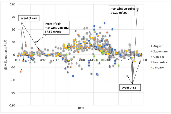
Figure 1.
Gaseous elemental mercury (GEM) fluxes (ng m−2 h−1) for all of the months during the day.
The measurement of mercury fluxes in the bibliography extend up to 88.90 ng m−2 h−1 in surface water, up to 46 ng m−2 h−1 in coastal sea and estuarine waters, up to 80 ng m−2 h−1 in open sea waters, from −375 ng m−2 h−1 up to 677 ng m−2 h−1 in wetlands and from −342 ng m−2 h−1 up to 517 ng m−2 h−1 in agricultural fields, as it is reviewed in [8]. In the Mediterranean area, the minimum values during the winter period were 0.70–2 ng m−2 h−1 and maximum values during the summer were 10–13 ng m−2 h−1 [35]. In another study, the values of mercury fluxes in Mediterranean open water extend up to 40.50 ng m−2 h−1 [10].
The GEM concentrations during the whole period of measurements ranged from 0.63 ng m−3 to 4.44 ng m−3 and the mean value was 1.04 ng m−3. Higher GEM concentrations were found during the summer. Increased wind velocities were observed in October in comparison with the other months, when the more peak events of GEM fluxes are observed. In August, when the temperature is higher than the other sampling months, there are, along with October, a high number of peak events. The temperature and the relative humidity followed the normal levels of the seasons, with high temperature in summer and high relative humidity in fall and winter.
Pearson correlation coefficients were calculated between GEM fluxes and other parameters. There was no correlation between GEM fluxes and mean GEM concentrations of the lower and the middle sampling heights, wind velocity, air temperature and barometric pressure. Similar results with no significant correlations were also found between mercury fluxes and wind velocity and air temperature over a coastal saltmarsh [21]. Despite the non-existent correlation between GEM fluxes and wind velocity, in some cases, the high wind velocity seemed to contribute to medium to high in absolute value positive and negative GEM fluxes. There is negligible correlation of GEM fluxes with mean GEM concentrations of the upper height, relative humidity, sunlight and cloudiness. The level of concentration does not seem to influence the GEM fluxes in contrast with the GEM concentration difference between the lower and the upper sampling height, which is quite strong (0.56). Therefore, high GEM concentrations do not contribute to high GEM fluxes. Hg* is a scaling variable that is not correlated with GEM concentration, is negligibly correlated with GEM concentration difference and is correlated significantly in a negative way with GEM fluxes. The correlation between Hg* and GEM fluxes (−0.82) is much more significant than the near zero correlation between u* (friction velocity) and GEM fluxes. The u* was calculated both with eddy covariance and gradient method with similar results. This means that theoretically the Hg* plays a more important role than u* in the calculation of GEM fluxes. However, u* as a number is one order of magnitude greater than Hg*. Thus, the combination of these two defines the calculation of GEM fluxes. U* is the friction velocity and is always positive by definition, whereas Hg* is either negative or positive and gives the sign in the GEM fluxes. Furthermore, there is very small correlation with wind direction, although wind direction does not influence the sign and the level of GEM fluxes. According to Figure 2, when the wind comes from the sea (50°–180°), the GEM emissions and depositions range between −47.19 and 43.23 ng m−2 h−1.
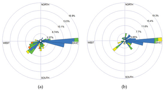
Figure 2.
Gaseous elemental mercury (GEM) fluxes rose plots for (a) emissions and (b) depositions. The GEM fluxes are divided in the following classes in absolute values: blue for 0-20 ng m−2 h−1, green for 20–40 ng m−2 h−1, yellow for 40–60 ng m−2 h−1, orange for 60–80 ng m−2 h−1 and red for fluxes greater than 80 ng m−2 h−1.
3.2. Diurnal Cycles
The most cases of events with high positive and low negative GEM fluxes were recorded from the morning until the evening, as it is shown in Figure 3. This could be a result of sunlight and increased temperature, which this study does not confirm because of the small related correlations. However, with more detailed examination, it is clear that all the peaks, positive and negative, during midday happen with intense sunlight and with very unstable atmospheric conditions. The temperature may be a possible factor that affects these events because at this time of the day the temperature is usually at its peak. Considering the time period between 9:00 a.m. to 7:00 p.m. and calculating correlations only for this time period, no differences arise. Concerning the emissions, the correlations of GEM fluxes with wind velocity, relative humidity and cloudiness are quite similar to the correlations for all the data, except for the correlation with sunlight and temperature, which are higher during midday. Regarding the depositions, the correlation with sunlight and temperature are negative and higher in absolute value than those of emissions. The correlation with the other parameters remains almost the same, with very low values. However, the fact that from the morning to the evening the temperature is increased, and there is sunlight, may drive to enhanced fluxes, in contrast with what happens in the evening. The study of [21] confirms that photochemistry may be the dominant factor that determines mercury volatilization from salt marsh sediments. As it is clear in Figure 3a, during the midday, the GEM emissions are particularly high with no low values, except in one case that the atmosphere is stable.
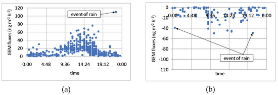
Figure 3.
Gaseous elemental mercury (GEM) fluxes (ng m−2 h−1) during the day for the entire period of measurements in (a) for emissions and (b) for depositions.
3.3. Atmospheric Stability
The atmospheric stability seems to affect the level of fluxes, as unstable conditions contribute to high fluxes in absolute value (see Table 2). The peak emissions and depositions are situated during midday when the atmosphere is unstable. The peak fluxes that were found at night are due to rain events. At night, the atmosphere is stable or neutral and, except for the rain events, the GEM fluxes are moving at low levels. In stable atmospheric conditions, the GEM fluxes extend from −24.79 ng m−2 h−1 to 25.46 ng m−2 h−1, excluding the rain events. During events of rain, it extends from −49.81 ng m−2 h−1 to 30.17 ng m−2 h−1. When Ri (Richardson number) ≥0.08 and L (Obukhov length) ≤77.12, GEM fluxes extend from −24.79 ng m−2 h−1 to 5.70 ng m−2 h−1 and, in very stable conditions (Ri ≥ 0.10 και L ≤40.56), it extends from −2.42 ng m−2 h−1 to 3.46 ng m−2 h−1. In a neutral atmosphere, the GEM fluxes are related with increased wind velocities and extend from −16.35 ng m−2 h−1 to 17.27 ng m−2 h−1, except for a single case of rain that has a value of 109.69 ng m−2 h−1. In unstable atmospheric conditions, the GEM fluxes coincide with the minimum (−50.30 ng m−2 h−1) and maximum (109.69 ng m−2 h−1) values and the fluxes between them. The unstable atmosphere favors the transport of air masses from other sites, as well as their mixing. With the use of the aerodynamic gradient method, the effect of ambient air turbulence in the amount of fluxes is clear here. Under a stable stratified atmospheric boundary layer at nighttime, the transport is based on molecular diffusion rather than on turbulent mixing [36].
3.4. Correlation with Energy Fluxes
There is near zero correlation between GEM fluxes and momentum fluxes, quite strong with sensible heat fluxes (0.42), slight with latent heat fluxes (0.24) and small correlation with net radiation (0.40). All of the energy fluxes were derived with the eddy covariance method. The plots between GEM fluxes and energy fluxes are shown in Figure 4. When we remove the peaks of GEM fluxes that are further away from the main group of values, the correlation coefficients with momentum and latent heat fluxes remain about the same and the correlation coefficients with sensible heat fluxes and net radiation are slightly increased. During a day, that there are mainly unstable atmospheric conditions, the GEM fluxes are mostly positive, the sensible heat fluxes, the latent heat fluxes and net radiation are also positive and high (see Table 1). During a night, that the atmospheric condition is stable and neutral, the GEM fluxes are either positive or negative but low in absolute value, the sensible heat fluxes and the net radiation are almost negative and the latent heat fluxes are mostly positive. When GEM fluxes are greater than 31.50 ng m−2 h−1, which happened during the period between 10:30 a.m. to 6:20 p.m., sensible heat fluxes are ≥30 W m−2, latent heat fluxes are ≥12 W m−2 and net radiation is ≥60 W m−2, except in a single case under a rain event (GEM flux: 109.69 ng m−2 h−1, sensible heat flux: −72.25 W m−2). According to [37], the surface–energy balance between radiation, sensible and latent heat fluxes determines the soil temperature and the temperature and humidity of air near the soil surface, which results in a correlation between solar radiation intensity and mercury fluxes. The soil–surface energy balance is influenced by solar radiation, atmospheric turbulence and other meteorological parameters.
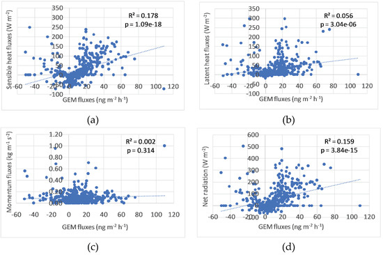
Figure 4.
Energy fluxes: (a) sensible heat fluxes; (b) latent heat fluxes; (c) momentum fluxes and (d) net radiation plotted against gaseous elemental mercury (GEM) fluxes.
3.5. Effects of Rain Events
Scattering of GEM fluxes for all the months during the day is represented in Figure 1, along with the rain events that happen in each case. Negative GEM fluxes that are related to rain events and measured right before or during the rain event cannot be explained by the deposition of elemental mercury, as mercury in rainwater mainly has the form of reactive-oxidized and particulate mercury. In addition, the vapor mercury instrument measures only elemental mercury. The possible explanations could be the transported mercury from a nearby area where the mercury evaporated from the soil due to the rain event or the co-precipitation of GEM with condensing water. The positive GEM fluxes follow the rain events with a time lag of a few minutes. A factor that contributes to the positive fluxes is the meteorological conditions, such as solar radiation, temperature and relative humidity, which may affect the conversion of Hg2+ to Hg0 on the soil and the rate of volatilization during and after wet deposition [38]. The volatile Hg0 that remains on the soil is induced to evade after the rain event due to the water and the humidity on the soil. According to [39], the increased fluxes of Hg0 from the bare soils during the precipitation and the peak in Hg0 emissions during the rain events are affected by the displacement of soil air pores containing Hg0 by rain water and the enhancement of Hg0 fluxes after the precipitation are dependent on soil moisture before the rain event, with greater flux a result of having drier soil. In our case, there are no increased positive fluxes during the rain events, but, right after these events, which is in agreement with [40], where except for the greater rate of Hg0 fluxes from desert soils, the emissions after the rainfall were one order of magnitude greater than those measured prior to the precipitation.
During the events of rain, the atmospheric stability is neutral or stable because of the time that the rain events happen. In addition, the relative humidity is enhanced and the wind velocity is also increased. Comparing the various rain events, it was noticed that the rain events in combination with increased wind velocity, even if the atmospheric condition is neutral and stable, have as a result higher positive and lower negative GEM fluxes. In addition, increased GEM concentrations are observed due to rain events. In the case of negative GEM fluxes, due to rain events, the GEM concentration at the highest sampling height presents a sudden increase and after the rain the GEM concentration at the lowest sampling height shows a sudden increase similar to that measured previously at the highest height.
3.6. Contributing Factors
The enhanced positive values of GEM fluxes could be explained by the special characteristics of Mediterranean Basin, such as high temperature and strong solar radiation that promote the photochemical reactions leading to higher Hg0 evasion from water to the atmosphere [41]. Furthermore, evasion of Hg0 over the vegetation is by a factor of ~10–15 greater than the fluxes over the water, as emergent macrophytes in a wetland contribute to the transport of Hg from soils to the atmosphere [42]. Salt-marsh plants, such as Halimione portulacoides that exists in our sampling area, enhance the vegetation-air Hg0 fluxes during daylight [43]. A daily trend was observed in [35], where the nighttime GEM evasion fluxes were 2 to 5-fold lower than those of the daytime, probably due to the lack of solar radiation that affects the release of elemental mercury from surface water during daytime. The negative sign in some cases is due to transported elemental mercury from other places. Dry deposition of Hg0, which is affected by plant uptake, is frequent at night over wet vegetation [42]. A large percentage of the Hg0 evasion from soil and sea is re-emitted Hg0 that had been previously deposited. The GEM deposition fluxes in the summer are affected mainly by local emissions and in the winter by long-range transport [44], which may contribute to the higher GEM fluxes in the fall and winter, as the transported mercury from polluted areas deposits and re-emits. The events with high positive and low negative GEM fluxes seem to occur more in the autumn than summer maybe due to higher wind velocity and more rain events. Seasonality in GEM fluxes due to the wind velocity was found in [45], where a wind velocity gas exchange model was used.
In most of the published work the model that is used in order to calculate air/water GEM fluxes is the two-layer gas exchange model using the Hg0 air concentration and the dissolved gaseous Hg0 concentration [46]. This model is highly affected by the variations of wind velocity [47]. According to [48], there is strong relationship between wind velocity and GEM fluxes and, according to [49], the GEM levels in the air–sea interface affect the GEM fluxes. In our case, the calculation of GEM fluxes is related to wind velocity and friction velocity in a low negligible extent, almost zero, as it was described above based on the correlation coefficients.
4. Conclusions
Gaseous elemental mercury (GEM) concentrations were measured in a coastal area that is surrounded by grassland, in northeastern Greece from August to November 2014 and January 2015. The GEM concentrations at three different heights in a micrometeorological tower were handled in order to calculate GEM fluxes based on the aerodynamic gradient method. The observed GEM fluxes were enlarged and positive during daytime, while, during nighttime, GEM fluxes were smaller and towards the surface for the most cases. Since solar radiation may affect the level of GEM concentrations and the evasion of mercury from surface water and grasslands, it can be reasonably assumed that the positive trend of GEM fluxes during daytime was favored by the high soil temperature and the high available energy occurring during summertime. Furthermore, the stability of the atmosphere is a strong factor influencing GEM fluxes, since unstable conditions under enhanced turbulent mixing during daytime can lead to increased GEM fluxes in absolute values. During nighttime, the transport is based on molecular diffusion that retains the GEM fluxes in low levels. Our area could be characterized as a source of elemental mercury, with evasion to be greater than deposition, with dry deposition of Hg0 being observed mainly during the night. The surrounding grassland is a strong factor that favours the enhanced positive GEM fluxes. Rain events are a strong contributing factor for enhanced GEM fluxes. Negative fluxes were recorded during the rain events and positive fluxes right after the rain events. The prevailing meteorological conditions expressed by measurements of wind velocity, temperature, relative humidity, sunlight and cloudiness did not drive the GEM fluxes linearly. There is not clear evidence that the wind velocity affects the GEM fluxes strongly, as the respective correlation with the fluxes is weak. In some cases, the high wind velocity may contribute to high positive and negative GEM fluxes, especially during rain events. Our research does not confirm the strong effect of wind velocity in GEM fluxes, as it arises in the two-layer gas exchange model that is used in a wide range for the calculation of GEM fluxes. Strong correlation was found between Hg* and GEM fluxes and a considerable positive correlation with GEM concentration difference between lower and upper sampling height. The level of concentrations does not affect the fluxes, as there is weak correlation between GEM concentration and GEM fluxes. Small positive correlations were observed between the GEM fluxes, net radiation and turbulent heat fluxes that were obtained by the eddy covariance method.
Author Contributions
C.P. carried out the field measurements, the data treatment and the interpretation of the data. S.R. and G.L. provided data analyses, data interpretation, authorship and editing of the publication. A.T. provided data of micrometeorological parameters and carried out calculations of energy fluxes.
Funding
This research received no external funding.
Acknowledgments
The Ph.D. thesis of Christiana Polyzou was internally funded by university funds.
Conflicts of Interest
The authors declare no conflict of interest.
References
- Rapsomanikis, S.; Weber, J.H. Methyl transfer reactions of environmental significance involving naturally occurring and synthetic reagents. In Organometallic Compounds in the Environment; Longmans Group Ltd.: Essex, UK, 1986; pp. 279–307. [Google Scholar]
- Fischer, R.; Rapsomanikis, S.; Andreae, M.O. Determination of methylmercury in fish samples using GC/AA and sodium tetraethylborate derivatization. Anal. Chem. 1993, 65, 763–766. [Google Scholar] [CrossRef] [PubMed]
- Fischer, R.G.; Rapsomanikis, S.; Andreae, M.O.; Baldi, F. Bioaccumulation of Methylmercury and Transformation of Inorganic Mercury by Macrofungi. Environ. Sci. Technol. 1995, 29, 993–999. [Google Scholar] [CrossRef] [PubMed]
- Lin, C.-J.; Pehkonen, S.O. The chemistry of atmospheric mercury: A review. Atmos. Environ. 1999, 33, 2067–2079. [Google Scholar] [CrossRef]
- Pirrone, N.; Cinnirella, S.; Feng, X.; Finkelman, R.B.; Friedli, H.R.; Leaner, J.; Mason, R.; Mukherjee, A.B.; Stracher, G.B.; Streets, D.G.; et al. Global mercury emissions to the atmosphere from anthropogenic and natural sources. Atmos. Chem. Phys. 2010, 10, 5951–5964. [Google Scholar] [CrossRef]
- Schroeder, W.H.; Munthe, J. Atmospheric mercury—An overview. Atmos. Environ. 1998, 32, 809–822. [Google Scholar] [CrossRef]
- Gustin, M.S. Exchange of Mercury between the Atmosphere and Terrestrial Ecosystems. In Environmental Chemistry and Toxicology of Mercury; John Wiley & Sons, Inc.: Hoboken, NJ, USA, 2011; pp. 423–451. [Google Scholar]
- Sommar, J.; Zhu, W.; Lin, C.-J.; Feng, X. Field Approaches to Measure Hg Exchange Between Natural Surfaces and the Atmosphere—A Review. Crit. Rev. Environ. Sci. Technol. 2013, 43, 1657–1739. [Google Scholar] [CrossRef]
- Zhu, W.; Sommar, J.; Lin, C.J.; Feng, X. Mercury vapor air–surface exchange measured by collocated micrometeorological and enclosure methods—Part I: Data comparability and method characteristics. Atmos. Chem. Phys. 2015, 15, 685–702. [Google Scholar] [CrossRef][Green Version]
- Gårdfeldt, K.; Sommar, J.; Ferrara, R.; Ceccarini, C.; Lanzillotta, E.; Munthe, J.; Wängberg, I.; Lindqvist, O.; Pirrone, N.; Sprovieri, F.; et al. Evasion of mercury from coastal and open waters of the Atlantic Ocean and the Mediterranean Sea. Atmos. Environ. 2003, 37 (Suppl. 1), 73–84. [Google Scholar] [CrossRef]
- Mason, R.P.; Lawson, N.M.; Lawrence, A.L.; Leaner, J.J.; Lee, J.G.; Sheu, G.-R. Mercury in the Chesapeake Bay. Mar. Chem. 1999, 65, 77–96. [Google Scholar] [CrossRef]
- Lindberg, S.E.; Dong, W.; Chanton, J.; Qualls, R.G.; Meyers, T. A mechanism for bimodal emission of gaseous mercury from aquatic macrophytes. Atmos. Environ. 2005, 39, 1289–1301. [Google Scholar] [CrossRef]
- Poissant, L.; Pilote, M.; Xu, X.; Zhang, H.; Beauvais, C. Atmospheric mercury speciation and deposition in the Bay St. François wetlands. J. Geophys. Res. Atmos. 2004, 109. [Google Scholar] [CrossRef]
- Zhang, H.H.; Poissant, L.; Xu, X.; Pilote, M. Explorative and innovative dynamic flux bag method development and testing for mercury air–vegetation gas exchange fluxes. Atmos. Environ. 2005, 39, 7481–7493. [Google Scholar] [CrossRef]
- Ferrara, R.; Mazzolai, B. A dynamic flux chamber to measure mercury emission from aquatic systems. Sci. Total Environ. 1998, 215, 51–57. [Google Scholar] [CrossRef]
- Ci, Z.; Zhang, X.; Wang, Z. Elemental mercury in coastal seawater of Yellow Sea, China: Temporal variation and air–sea exchange. Atmos. Environ. 2011, 45, 183–190. [Google Scholar] [CrossRef]
- Rolfhus, K.R.; Fitzgerald, W.F. The evasion and spatial/temporal distribution of mercury species in Long Island Sound, CT-NY. Geochim. Cosmochim. Acta 2001, 65, 407–418. [Google Scholar] [CrossRef]
- Liss, P.S.; Merlivat, L. Air-Sea Gas Exchange Rates: Introduction and Synthesis. In The Role of Air-Sea Exchange in Geochemical Cycling; Buat-Ménard, P., Ed.; Springer: Dordrecht, The Netherlands, 1986; pp. 113–127. [Google Scholar]
- Wanninkhof, R. Relationship Between Wind Speed and Gas Exchange Over the Ocean. J. Geophys. Res. 1992, 97, 7373–7382. [Google Scholar] [CrossRef]
- Lee, X.; Benoit, G.; Hu, X. Total gaseous mercury concentration and flux over a coastal saltmarsh vegetation in Connecticut, USA. Atmos. Environ. 2000, 34, 4205–4213. [Google Scholar] [CrossRef]
- Smith, L.M.; Reinfelder, J.R. Mercury volatilization from salt marsh sediments. J. Geophys. Res. Biogeosci. 2009, 114. [Google Scholar] [CrossRef]
- Trepekli, A.; Loupa, G.; Rapsomanikis, S. Seasonal evapotranspiration, energy fluxes and turbulence variance characteristics of a Mediterranean coastal grassland. Agric. For. Meteorol. 2016, 226–227, 13–27. [Google Scholar] [CrossRef]
- Tekran. Available online: https://www.tekran.com/products/ambient-air/tekran-model-2537-cvafs-automated-mercury-analyzer/ (accessed on 10 July 2019).
- Kim, K.-H.; Kim, M.-Y. The exchange of gaseous mercury across soil–air interface in a residential area of Seoul, Korea. Atmos. Environ. 1999, 33, 3153–3165. [Google Scholar] [CrossRef]
- Baldocchi, D. University of California, Berkeley, Biometeorology Lab, ESPM 228, Advanced Topics in Biometeorology and Micrometeorology: Lecture 2 on Micrometeorological Flux Measurement Methods/Flux-Gradient Theory. Available online: https://nature.berkeley.edu/biometlab/espm228/Lecture_2_Notes_ESPM_228_Flux_Gradient_Theory_v2016.pdf (accessed on 10 July 2019).
- Wesely, M.L.; Hicks, B.B. A review of the current status of knowledge on dry deposition. Atmos. Environ. 2000, 34, 2261–2282. [Google Scholar] [CrossRef]
- Rapsomanikis, S.; Trepekli, A.; Loupa, G.; Polyzou, C. Vertical Energy and Momentum Fluxes in the Centre of Athens, Greece During a Heatwave Period (Thermopolis 2009 Campaign). Bound. Layer Meteorol. 2015, 154, 497–512. [Google Scholar] [CrossRef]
- Oke, T.R. Boundary Layer Climates, 2nd ed.; University Press: Cambridge, UK, 1987; 464p. [Google Scholar]
- Monin, A.S.; Obukhov, A.M. Basic Laws of Turbulent Mixing in the Atmosphere Near the Ground. Tr. Akad. Nauk SSSR Geoph. Inst. 1954, 24, 163–187. [Google Scholar]
- MATLAB and Statistics Toolbox Release 2010b; The MathWorks, Inc.: Natick, MA, USA, 2010.
- Foken, T. Micrometeorology; Springer: Berlin/Heidelberg Germany, 2008; p. 308. [Google Scholar]
- Zhu, W.; Sommar, J.; Lin, C.J.; Feng, X. Mercury vapor air–surface exchange measured by collocated micrometeorological and enclosure methods—Part II: Bias and uncertainty analysis. Atmos. Chem. Phys. 2015, 15, 5359–5376. [Google Scholar] [CrossRef]
- Hsieh, C.-I.; Katul, G.; Chi, T.-W. An approximate analytical model for footprint estimation of scalar fluxes in thermally stratified atmospheric flows. Adv. Water Resour. 2000, 23, 765–772. [Google Scholar] [CrossRef]
- Gårdfeldt, K.; Feng, X.; Sommar, J.; Lindqvist, O. Total gaseous mercury exchange between air and water at river and sea surfaces in Swedish coastal regions. Atmos. Environ. 2001, 35, 3027–3038. [Google Scholar] [CrossRef]
- Ferrara, R.; Mazzolai, B.; Lanzillotta, E.; Nucaro, E.; Pirrone, N. Temporal trends in gaseous mercury evasion from the Mediterranean seawaters. Sci. Total Environ. 2000, 259, 183–190. [Google Scholar] [CrossRef]
- Kim, K.-H.; Lindberg, S.E.; Meyers, T.P. Micrometeorological measurements of mercury vapor fluxes over background forest soils in eastern Tennessee. Atmos. Environ. 1995, 29, 267–282. [Google Scholar] [CrossRef]
- Scholtz, M.T.; Van Heyst, B.J.; Schroeder, W.H. Modelling of mercury emissions from background soils. Sci. Total Environ. 2003, 304, 185–207. [Google Scholar] [CrossRef]
- Ariya, P.A.; Amyot, M.; Dastoor, A.; Deeds, D.; Feinberg, A.; Kos, G.; Poulain, A.; Ryjkov, A.; Semeniuk, K.; Subir, M.; et al. Mercury Physicochemical and Biogeochemical Transformation in the Atmosphere and at Atmospheric Interfaces: A Review and Future Directions. Chem. Rev. 2015, 115, 3760–3802. [Google Scholar] [CrossRef]
- Song, X.; Van Heyst, B. Volatilization of mercury from soils in response to simulated precipitation. Atmos. Environ. 2005, 39, 7494–7505. [Google Scholar] [CrossRef]
- Lindberg, S.E.; Zhang, H.; Gustin, M.; Vette, A.; Marsik, F.; Owens, J.; Casimir, A.; Ebinghaus, R.; Edwards, G.; Fitzgerald, C.; et al. Increases in mercury emissions from desert soils in response to rainfall and irrigation. J. Geophys. Res. Atmos. 1999, 104, 21879–21888. [Google Scholar] [CrossRef]
- Kotnik, J.; Sprovieri, F.; Ogrinc, N.; Horvat, M.; Pirrone, N. Mercury in the Mediterranean, part I: Spatial and temporal trends. Environ. Sci. Pollut. Res. 2014, 21, 4063–4080. [Google Scholar] [CrossRef] [PubMed]
- Lindberg, S.E.; Meyers, T.P. Development of an automated micrometeorological method for measuring the emission of mercury vapor from wetland vegetation. Wetl. Ecol. Manag. 2001, 9, 333–347. [Google Scholar] [CrossRef]
- Canário, J.; Poissant, L.; Pilote, M.; Caetano, M.; Hintelmann, H.; O’Driscoll, N.J. Salt-marsh plants as potential sources of Hg0 into the atmosphere. Atmos. Environ. 2017, 152, 458–464. [Google Scholar] [CrossRef]
- Gencarelli, C.N.; De Simone, F.; Hedgecock, I.M.; Sprovieri, F.; Yang, X.; Pirrone, N. European and Mediterranean mercury modelling: Local and long-range contributions to the deposition flux. Atmos. Environ. 2015, 117, 162–168. [Google Scholar] [CrossRef]
- Marumoto, K.; Imai, S. Determination of dissolved gaseous mercury in seawater of Minamata Bay and estimation for mercury exchange across air–sea interface. Mar. Chem. 2015, 168, 9–17. [Google Scholar] [CrossRef]
- Liss, P.S.; Slater, P.G. Flux of Gases across the Air-Sea Interface. Nature 1974, 247, 181–184. [Google Scholar] [CrossRef]
- Ci, Z.; Wang, C.; Wang, Z.; Zhang, X. Elemental mercury (Hg(0)) in air and surface water of the Yellow Sea during late spring and late fall 2012: Concentration, spatial-temporal distribution and air/sea flux. Chemosphere 2015, 119, 199–208. [Google Scholar] [CrossRef]
- Wang, C.; Ci, Z.; Wang, Z.; Zhang, X. Air-sea exchange of gaseous mercury in the East China Sea. Environ. Pollut. 2016, 212, 535–543. [Google Scholar] [CrossRef]
- Andersson, M.E.; Sommar, J.; Gårdfeldt, K.; Jutterström, S. Air–sea exchange of volatile mercury in the North Atlantic Ocean. Mar. Chem. 2011, 125, 1–7. [Google Scholar] [CrossRef]
© 2019 by the authors. Licensee MDPI, Basel, Switzerland. This article is an open access article distributed under the terms and conditions of the Creative Commons Attribution (CC BY) license (http://creativecommons.org/licenses/by/4.0/).