Impact of Urban Growth on Air Quality in Indian Cities Using Hierarchical Bayesian Approach

Abstract

Several studies have found rising ambient particulate matter (PM${}_{2.5}$) concentrations in urban areas across developing countries. For setting mitigation policies source-contribution is needed, which is calculated mostly through computationally intensive chemical transport models or manpower intensive source apportionment studies. Data based approach that use remote sensing datasets can help reduce this challenge, specially in developing countries which lack spatially and temporally dense air quality monitoring networks. Our objective was identifying relative contribution of urban emission sources to monthly PM${}_{2.5}$ ambient concentrations and assessing whether urban expansion can explain rise of PM${}_{2.5}$ ambient concentration from 2001 to 2015 in 15 Indian cities. We adapted the Intergovernmental Panel on Climate Change’s (IPCC) emission framework in a land use regression (LUR) model to estimate concentrations by statistically modeling the impact of urban growth on aerosol concentrations with the help of remote sensing datasets. Contribution to concentration from six key sources (residential, industrial, commercial, crop fires, brick kiln and vehicles) was estimated by inverse distance weighting of their emissions in the land-use regression model. A hierarchical Bayesian approach was used to account for the random effects due to the heterogeneous emitting sources in the 15 cities. Long-term ambient PM${}_{2.5}$ concentration from 2001 to 2015, was represented by a indicator R (varying from 0 to 100), decomposed from MODIS (Moderate Resolution Imaging Spectroradiometer) derived AOD (aerosol optical depth) and angstrom exponent datasets. The model was trained on annual-level spatial land-use distribution and technological advancement data and the monthly-level emission activity of 2001 and 2011 over each location to predict monthly R. The results suggest that above the central portion of a city, concentration due to primary PM${}_{2.5}$ emission is contributed mostly by residential areas (35.0 ± 11.9%), brick kilns (11.7 ± 5.2%) and industries (4.2 ± 2.8%). The model performed moderately for most cities (median correlation for out of time validation was 0.52), especially when assumed changes in seasonal emissions for each source reflected actual seasonal changes in emissions. The results suggest the need for policies focusing on emissions from residential regions and brick kilns. The relative order of the contributions estimated by this study is consistent with other recent studies and a contribution of up to 42.8 ± 14.1% is attributed to the formation of secondary aerosol, long-range transport and unaccounted sources in surrounding regions. The strength of this approach is to be able to estimate the contribution of urban growth to primary aerosols statistically with a relatively low computation cost compared to the more accurate but computationally expensive chemical transport based models. This remote sensing based approach is especially useful in locations without emission inventory.

1. Introduction

1.1. Background

Researches have shown that over a long-term time scale, pollutant concentrations simulated from dispersion models are correlated with satellite-sensor retrieved columnar depths. Such correlations have been found between modeled PM${}_{2.5}$ and satellite-sensor retrieved aerosol optical depth (AOD) [1] as well as between modeled SO${}_2$ ground emissions and satellite vertical column density Itahashi et al. [2]. However this proportionality may not hold true if emission inventory is out-of-date or unrepresentative of ground sources. An example of this was provided by Akimoto et al. [3] who observed increasing tropospheric NO${}_2$ from satellite but decreasing emissions from coal consumption inventory estimates. Similarly de Meij et al. [4] found high spatial agreement of aerosol precursor gases from European inventories (EMEP and AEROCOM) with MODIS sensor based AOD retrievals but also found that large differences in simulated surface concentrations are not reflected well within AOD retrievals. de Meij et al. [4] suggested that highly temporal emissions do not strongly impact aerosol concentrations and they concluded that seasonal temporal variation is more important than daily or weekly temporal distribution. Therefore in developing countries which are undergoing rapid economic development and urban growth the emission inventories may be out of date and pollutant concentration derived solely from emission inventories using chemical transport modeling can be unreliable. It is necessary to thus explore the use of alternative schemes that can consider changes in land-use growth for modeling the concentrations.

Statistical approaches like land use regression (LUR) models present an attractive alternative to the emission based chemical transport models, as they have low computation costs [5] and employ explanatory variables constructed from easily obtainable data [6]. They were first developed in late 1990s’s [7,8] mainly for mapping traffic related pollution like NO${}_2$. Since then LUR along with geographic weighted regression (GWR) models have been used as a computationally cost-effective method for mapping primary and secondary formed pollutants to explain spatio-temporal variation in the concentrations due to geographic factors. Recently interest is surging to develop LUR models for PM${}_{2.5}$ [9,10,11,12,13] due to the cognizance of its effect on human health [14] and its rising concentration across developing countries [15]. Van Donkelaar et al. [16] showed that using land-use in GWR to observed and simulated AOD and ambient PM${}_{2.5}$ concentrations results in significant PM${}_{2.5}$ concentration prediction in locations lacking ground observations. Land-use changes or urban growth itself could be responsible for rising concentration. For example, Zhou et al. [12] undertook observations of 190 Chinese cities in 2014 and found that socio-economic and land-use variables, such as population density, industrial structure and road density increase PM${}_{2.5}$ concentration level while per capita GDP (gross domestic product) improves air quality. Similarly Lin et al. [10] found PM${}_{2.5}$ concentration was driven by population, local economic growth and urban area growth. Some researches have also described contribution of the land-use predictor variables in explaining the pollutant concentration [17,18]. These relative contributions can be useful for designing evidence based policies where land-use emission inventories or emission factors have not been established. Currently Indian cities are experiencing degraded air quality due to intense economic development and in the future, air quality management will become more challenging. Yet, literature is scarce about utilizing statistical approaches in India and only recently LUR [19,20] or multiple linear regression [21] have been attempted. This is probably due to limited availability of land-use data for Indian cities, similar to other developing countries. Thus, there is a need to investigate whether areal growth in remote sensing derived land-use classes could explain rising PM${}_{2.5}$ concentrations. This would also be useful for identifying which land-use type contributes the most to urban PM${}_{2.5}$ concentrations.

1.2. Objective

The goal of this research is to estimate the impact on long-term (2001 to 2015) PM${}_{2.5}$ concentrations due to urban growth in 15 Indian cities with LUR model using remote sensing and meteorological datasets. The specific objective is to calculate relative contribution of the land-use and vehicular sources to urban fine aerosol concentration and compare the results with non-remote sensing based estimations. The originality of our LUR based model is the adaption of IPCC emission framework which allows explicit accounting of policy changes in the form of urban expansion and technological advancement as well as seasonal variation in emissions. Furthermore, we have used spatially distributed land-use types derived from publicly available satellite datasets which can be updated rapidly with urban growth compared to emission inventory.

2. Methodology

The flowchart of dataset and methodology employed for estimating emission parameters is shown in Figure 1. Within India, 9 cities with the highest PM${}_{2.5}$ World Health Organization [22] concentration and the 6 megacities were chosen for this study. They are collectively referred to as ‘Tier-2’ and ‘Tier-1’ city respectively. Tier-1 cities, also known as megacities, have higher per-capita gross domestic product (GDP) and population compared to Tier-2 cities. Correspondingly, Tier-1 cities tend to have more manufacturing industries compared to Tier-2 cities. All the 15 cities are shown geographically in Figure 2. Average population of Tier-1 and Tier-2 cities in 2010 was 13.3 million and 2.3 million respectively while the average per-capita GDP was 1700 USD and 1100 USD respectively.

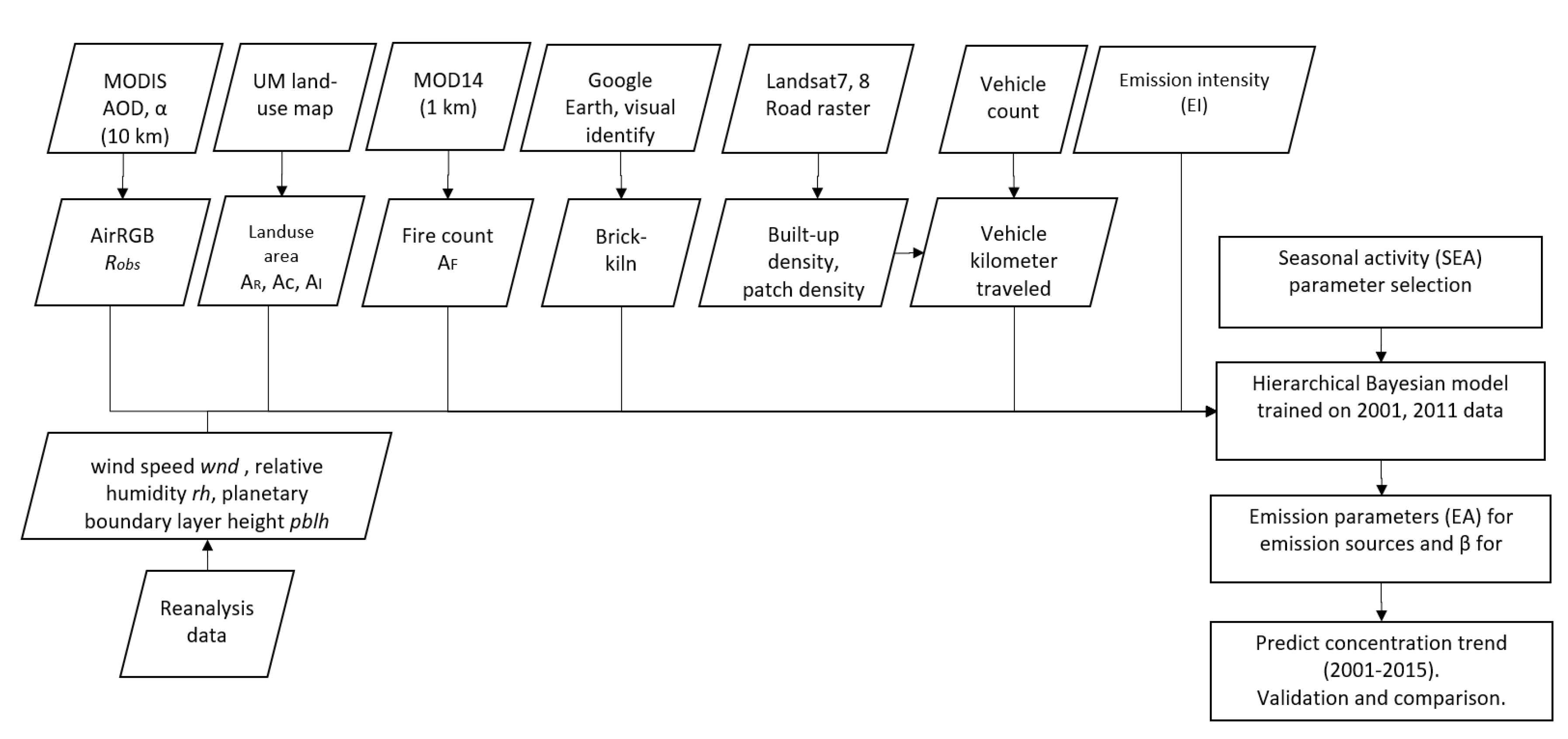
2.1. Conceptual Framework

Kaya identity [23] states: $Emission=energyconsumption\times emissionfactor$. To estimate anthropogenic emission of pollutants from emission sectors, emission inventories use its modified form [24], where emission factor is defined as emission per unit consumption of energy. Total emissions, E, from emitting source sectors $sc$ and vehicles V is shown in Equation (1) [25,26].

$$E=\sum _{sc}^{}{C}_{sc}·E{F}_{sc}·(1-ef{f}_{sc})+\sum _v^{}{A}_V·VK{T}_V·E{F}_v$$

(1)

where, C is a sector’s energy consumption, $EF$ the unabated emission factor and $eff$ the fuel efficiency. For vehicle of type V with a count of $A_V$, $VKT$ is its monthly distance traveled in kilometers.

Several inventories exist with regards to black carbon, SO${}_2$ and PM${}_{2.5}$ anthropogenic emissions over Asian countries. The most spatially comprehensive inventory is Regional Emission inventory in ASia (REASv2) [26]. Since many countries do not have updated emission inventories, the emission factors are ‘borrowed’ from some other country and the energy consumption is estimated statistically. However the borrowed emission factors may not represent the emission sources or source emission strengths that are unique to that country. Within Asia, country level emission factors (EF) are mostly available for Japan, China, Taiwan, South Korea and India [25,26]. In India, several inventories have been prepared at country level [27,28] or for specific districts [29,30,31,32] but only a few have considered primary PM${}_{2.5}$ emissions. Furthermore, emissions are dependent on seasonal activity of the emission sources and only few inventories [26,33] have explicitly considered this, for example, brick kilns are active only during the dry season from October to June [34]; crop residue burning is prominent during the two harvesting months of Rabi crop (April-May) and Kharif crop (October-November) [35]. In addition, emissions are affected not only by scale of production but also the production technology as it acts along with population and affluence in a multiplicative manner [36]. Although measuring or quantifying the state of technology is itself major research challenge [37], decreasing CO${}_2$ emission intensity can be an indicator of overall status of technological evolution [38]. The World Resource Institute also suggests that pollution intensity of production (defined as ratio of emission and gross national product) can be a possible a technological indicator.

Based on this, carbon emission intensity was used to depict the state of technology in this research. Sector $sc$ was segregated into land-use type $LU$. We modified Equation (1) to represent emission from any $LU$ in a month $mon$ and year $yr$ as the product of total area under a $LU$ type, its mean monthly per unit area emission in the base year $base$, technological evolution in $yr$ with respect to the base year $base$ and a coefficient to account for seasonal variation in emissions based on $mon$. Base year, $base$, is the reference year from which technological evolution in a year $yr$ can be compared. The key emission sources considered included land-use $LU$ (residential—R, commercial—C, industrial—I, brick kiln—$BK$, agricultural crop fire—$agro$) and vehicles V. Total emissions E from the key sources in a month, $mon$, of year, $yr$, was formulated as Equation (2).

$$E(yr,mon)=\sum _{LU}^{}{A}_{LU}\left(yr\right)·E{I}_{LU}\left(yr\right)·E{C}_{LU}·SE{A}_{LU,mon}+A_V\left(yr\right)·VKT·E{I}_V\left(yr\right)·E{C}_V·SE{A}_{V,mon}$$

(2)

In Equation (2), A is the number of units of each emission source such that it refers to the total area (in m${}^2$) in the case of area sources (e.g., residential, commercial and industries) or total count in the case of point sources (e.g., brick kilns, crop-fires and vehicles). $EC$ is emission coefficient of each emission source type in the base year and can be interpreted as corresponding to mean monthly emission of the emission source. Yearly technological evolution in $EC$ is represented by $EI$, ratio of annual emission intensity in year $yr$ to that of the base year. $SE{A}_{mon}$ is a coefficient varying between 0 to 1 to account for relative monthly variation in emissions from $LU$ or V. The seasonal emission activity $SEA$ takes on a value between 0 and 1 for each month. It is assumed to be 1 during the month relative monthly emission activity is maximum and $SEA$ is assumed to be 0 when the emission source is not emitting at all. Thus, emission from each unit of $LU$ type in any month $mon$ of the year $yr$ is a product of its emission coefficient $EC$ in the base year scaled by technological evolution $EI$ in year $yr$ and corrected by seasonal emission activity $SE{A}_{mon}$.

2.2. Data Used

2.2.1. Fine Aerosol Concentration Indicator

In this paper air quality is meant to refer PM${}_{2.5}$ concentrations because cities in India, like many other developing countries, have much higher than acceptable level for PM${}_{2.5}$ than other pollutants commonly used for judging air quality (e.g., SO${}_2$, NO${}_2$, CO and O${}_3$). PM${}_{2.5}$ refers to particles with aerodynamic diameter less than 2.5 $\mathsf{\mu }$m and is found to be fine mode atmospheric aerosols. PM${}_{2.5}$ particles are produced by primary emissions or through gas-to-particle conversions. A high PM${}_{2.5}$ mass concentration changes aerosol parameters causing high aerosol optical depth (AOD) and angstrom exponent (>0.8) values. Due to lack of dense spatio-temporal ground based PM${}_{2.5}$ measurements, satellite retrieved AOD and angstrom exponent has been used to estimate PM${}_{2.5}$ [1,39]. The major disadvantage with satellite based retrievals is that they represent columnar values and require other ancillary meteorological information on boundary layer height and relative humidity for estimating surface PM${}_{2.5}$. Under suitable conditions, such as a well-mixed boundary layer and low ambient relative humidity, correlation between daily PM${}_{2.5}$ mass concentrations and satellite AOD can be as high as 0.9 [40].

Gridded AOD and angstrom exponent values at 10 km spatial resolution are available from ‘MOD04L2 Collection6’ product of MODIS (Moderate Resolution Imaging Spectroradiometer) sensor onboard NASA’s Earth Observing System (EOS) Terra satellite. In an earlier paper, Misra et al. [15] developed a scheme (called ‘AirRGB’) to mathematically decompose AOD and angstrom exponent values into three unitless components for characterizing urban air quality. The decomposition was based on thresholds determined from mean annual AOD and angstrom exponent values from 60 cities around the world. One of the AirRGB components—called R—corresponds to high PM${}_{2.5}$ concentrations on a scale of 0 to 100. R takes on a value of 100 when a high AOD (0.6) and a high angstrom exponent (0.8) value is retrieved, and R is 0 when either or both AOD and the angstrom exponent are low (0.05). R has been demonstrated to correspond to ambient PM${}_{2.5}$ concentrations with a high coefficient of agreement (0.97) [15] and was used in this research as an indicator for PM${}_{2.5}$ concentration. For reference, a binned PM${}_{2.5}$ concentration between 0 to 25 $\mathsf{\mu }$g/m${}^3$ corresponds to a mean R of 13.12 and PM${}_{2.5}$ between 176 to 200 $\mathsf{\mu }$g/m${}^3$ corresponds to a mean R of 95.47 Misra et al. [15]. The uncertainty in R is estimated as ±15.98 owing to the uncertainty in MODIS based AOD and angstrom exponent retrievals [41].

A similar decomposition scheme was considered in this research to obtain continuous spatio-temporal representation of ambient PM${}_{2.5}$ concentrations. R was obtained by applying AirRGB scheme to daily MOD04L2 imagery from 2001 to 2015 and their mean monthly composites were used. Indian cities often have a higher AOD and angstrom exponent than what was considered while deriving the original AirRGB thresholds [15]. So, to prevent saturation of R at 100, the original AirRGB threshold for AOD and angstrom exponent was revised from 0.6 and 0.8 to 1.5 and 1.0, respectively. Several daily satellite retrievals were missing due to cloud coverage during the monsoon months (June, July and August). Techniques like spatially sliding windows [42], n-day composites on a rolling basis [43] or pixel coverage threshold monthly mean [44] have been used previously to interpolate missing values. However the final values can vary by as much as 30% and neither technique has been judged to be superior [44]. Furthermore, on monthly and yearly scales, bias towards clear-sky values has not been found to be significant [45]. In this research, missing R values were interpolated temporally by considering rolling mean of 15-day R values. Further discussion on the effect of missing values on the AOD mean is provided in Section 1.1 and Figure S1 in Supplementary Materials.

Furthermore, AOD increases when relative humidity increases, due to aerosol hygroscopic growth [46]. Therefore, R was also corrected for hygroscopic growth using the approach suggested by Chin et al. [47], as shown in Equation (3). Where, $R_{obs}$ refers to the R corrected for relative humidity, and $\beta \left(rh\right)$ is the mass extinction coefficient that characterizes hygroscopic aerosol at different relative humidity ($rh$) values [47] for different aerosol types, such as, sulfate sea-salt, black carbon and organic carbon. Water-soluble aerosols have the highest mass concentration in northern India [48] with sulfates being the most common water soluble aerosol [49]. Consequently, the $\beta \left(rh\right)$ of sulfate aerosol [47], was applied for hygroscopic correction. The $R_{obs}$ trend over the central pixel of study locations is shown in Figure 3 where an increasing trend can be seen from 2001.

$$R_{obs}=\frac{R}{\beta \left(rh\right)}$$

(3)

2.2.2. Urban Land-Use and Expansion

Residential, commercial and industrial regions are the key area emission sources in cities. Emission may take place from municipal waste-combustion, residential and commercial cooking, use of diesel based electricity generators, and others [30,50]. Like many developing countries, land-use data is not publicly available for most cities in India. Sritarapipat and Takeuchi [51] proposed the technique of identifying spatial land-use morphology in terms of residential, commercial and industrial areas by using remote sensing derived building heights and nighttime light. This approach was followed to obtain the spatial distribution of emission sources. Open digital surface models at 30 m resolution, AW3D30 [52] and ASTER GDEMv2 [53] were used for deriving the height of built structures [54] for the years 2011 and 2001, respectively. Upsampled nighttime day-night band (DNB) of VIIRS dataset was used to obtain the nighttime light. As AW3D30 and ASTER GDEMv2 are the only two DSM datasets that are publicly available at 30 m resolution currently, urban land-use were prepared only for these snapshot times. Due to this spatial distribution of residential, commercial and industrial could only be identified for 2001 and 2011. The minimum user accuracy of residential and commercial area in these cities being more than 64% and minimum user accuracy for industrial being 72%. To overcome the limited availability of land-use data in studying their long-term contributions, population and per-capita GDP values for each city was used for interpolation to obtain total areas of residential ($A_R$), commercial ($A_C$) and industrial ($A_I$) structures from 2001 to 2015 [55]. This was based on the finding that urban expansion is governed by socio-economic development in the form of population and per capita GDP [56]. District level population and capita GDP values were obtained from statistical data sources [57,58].

2.2.3. Agricultural Fires

The burning of crop residue is a seasonal activity, the emitted particles from which can travel great distances and affect several cities after the harvest of rice or wheat crops in India. Daily fire count from the MODIS thermal anomalies product (MOD14) [59] aboard NASA’s Terra satellite was used for indicating crop residue burning [60]. It is available at the daily level with a 1 km spatial resolution since 2001. MOD14 is known to underestimate fire counts in October and November over northern India [35]. The daily fire counts within 300 km of a North Indian city and a South Indian city are compared in Figure 4. In northern India, bimodal distribution peaking during April to May and October to November can be seen clearly owing to wheat-rice double cropping systems. The city with the most fire counts was Ludhiana. Other northern Indian cities like Kanpur or Jaipur had around a tenth of fire counts compared to Ludhiana. On an average cities in northern India also showed the highest incidences of fire occurrence (3 to 20 times compared to those in West or South). Unlike northern Indian cities, peaks are unimodal in southern Indian cities and occur around March-April. In this research, the monthly mean of daily fire counts within 500 km of each study site was considered for this purpose and designated as $A_{agro}$.

2.2.4. Brick Kiln

Brick kilns are construction-brick making factories that emit high amounts of black carbon, PM${}_{2.5}$ and SO${}_2$ while they operate during the dry season [34]. Official estimate of the number of brick kilns in India is unavailable and they are assumed to be more than 100,000 [34]. Brick kilns are often found around the periphery of urbanizing cities and can be spotted in high resolution imagery due to their distinct appearance [61]. They were visually identified around the study sites using Google Earth imagery. Approximately 3000 brick kilns were located beyond 40 km and within 70 km radius of New Delhi, mostly along the riverbed. For other cities, the number of brick kilns was comparatively lower but they were also found beyond 20 km and within 60 km radius from the city center. Based on visual interpretation approximate number of the brick kilns, $A_{BK}$, was assigned as (a) Low: 50 brick kilns, (b) Mid: 50–200 brick kilns and (c) High: 400 brick kilns.

2.2.5. Vehicle Kilometers Traveled (VKT)

Both vehicle population and vehicle kilometers traveled (VKT) affect total vehicular emissions, as formulated in several emission inventories [26,62] and as shown in Equation (1). Vehicle population is available annually for each major city in India from Ministry of Road Transport and Highways [63]. However annual VKT with a consistent calculation approach is available only for Bangalore, New Delhi and Kolkata as 8634 km, 9594 km and 7230 km respectively [64]. VKT for other cities was calculated by following the argument that VKT is influenced by urban sprawl [65,66]. Urban form can be characterized by: normalized built-up density(nBD), normalized landscape shape index(nLSI), normalized largest patch index (nLPI), normalized patch density (nPD), and normalized edge density (nED) [67]. These shape metrics were calculated for the built-up land-cover class by classifying Landsat 8 imagery for the year 2013 for each location. Thereafter correlation of the reported VKT was computed with each urban form metric as shown in Figure 5. Based on the strong inverse correlation between VKT and nLPI ($R^2$ = 0.95) and nBD ($R^2$ = 0.88), an empirical equation (Equation (4)) was formulated to estimate VKT for any other city s by using the built-up density of Bangalore city as reference. Thereafter VKT was allocated proportionately to grid level, $VK{T}_k$, on the basis of length of major road section lying within each cell, k, of the grid. The grid size was chosen as 10 km × 10 km to keep it consistent with grid of R. Openly available road network shapefile [68] was used for this purpose.

$$VK{T}_s=\frac{1.7769-nLP{I}_s}{0.0002}.\frac{nB{D}_s}{nB{D}_{Bangalore}}$$

(4)

2.2.6. Emission Intensity

For India’s yearly carbon emission intensity, $E{I}_{yr}$ statistics are available at a national level for manufacturing, construction, waste and transport sectors from the World Resource Institute through its ‘Climate Data Explorer’ platform. Technological evolution in year $yr$ was depicted with respect to the base year as 2001, $EI\left(yr\right)$ was formulated as a ratio shown in Equation (5). As mentioned earlier, 2001 was considered as the base year and likewise $EI\left(yr\right)$ was calculated with respected to the $E{I}_{base}$.

$$EI\left(yr\right)=\frac{E{I}_{y}r}{E{I}_{base}}$$

(5)

Summary of the emission sources used in this research is shown in

Table 1. Summary of emission sources considered. A refers to the total area in case of land-use sources ($LU$) or to the total vehicle population in case of vehicles, $EI$ refers to emission intensity and $EC$ refers to emission coefficient.

Emission Source	Estimation Method and Data Source	Temporal Availability	Emission Formulation
Residential, Commercial, Industrial	Classification of AW3D30 and ASTER derived building height and VIIRS DNB	Spatial distribution for 2001 and 2011, annually interpolated total area for other years	$A_R·E{I}_R·E{C}_R$, $A_C·E{I}_C·E{C}_C$, $A_I·E{I}_I·E{C}_I$
Agricultural fires	Thermal anomalies in MOD14 within 300 km from city considered	Daily aggregated to monthly level (2001 to 2015)	$A_{agro}·E{I}_{agro}·E{C}_{agro}$
Brick kilns	Visual identification in Google Earth maps	One-time counts for 2015	$A_{BK}·E{I}_{BK}·E{C}_{BK}$
Vehicle	Vehicle population from Year Book, VKT from literature and Landsat derived nLPI and nBD	Annual (2001 to 2015)	$A_V·VKT·E{I}_V·E{C}_V$

.

2.2.7. Seasonal Emission Activity

It is well known that monthly emissions depend on the source seasonal activity [26,32,33], for example, vehicles undergo cold start emission during winters, diesel-based electricity generators are used to offset power-cuts by residences and commercial entities like offices or hospitals during summers, brick kilns operate only during dry season, residential areas burn wood for heating during winter season, and so forth. While crop residue burning activity can be inferred directly from satellite based fire count products, emission activity for other sources is based on consumption based statistics. So far, only Kurokawa et al. [26] and Paliwal et al. [33] have shared the monthly variation of emission activity for India. Kurokawa et al. [26] shared the logical basis of using monthly electricity and energy consumption to characterize seasonal activity for domestic and road emissions over India. Same monthly activity variation was ascribed throughout India in the REASv2, which may not be true owing to diverse climates within the country. $SEA$ for the colder months such as, November, December and January is designated as 1 to indicate that monthly emission activity is maximum during these months. Owing to a lack of seasonal emission activity data for each source, we derived these statistically for summer and rain seasons. They were denoted as $s,r$ respectively as shown in

Table 2. Assumed monthly distribution of seasonal activity parameters ($SE{A}_{mon}$). $s,r$ represent values of seasonal activity for summer and rain season respectively. For any source $SE{A}_{mon}$ represents ratio of emissions in any month $mon$ compared to its maximum monthly emission.

Source	January	February	March	April	May	June	July	August	September	October	November	December
Residential ($A_R$)	1	$\frac{2+s}{3}$	$\frac{1+s}{2}$	s	s	$\frac{s+r}{2}$	r	r	r	$\frac{r+1}{2}$	1	1
Commercial ($A_C$)	1	$\frac{2+s}{3}$	$\frac{1+s}{2}$	s	s	$\frac{s+r}{2}$	r	r	r	$\frac{r+1}{2}$	1	1
Industrial ($A_I$)	1	1	1	1	1	1	1	1	1	1	1	1
Crop fire ($A_{agro}$)	1	1	1	1	1	1	1	1	1	1	1	1
Brick-kiln ($A_{BK}$)	1	1	1	1	1	0	0	0	0	1	1	1
Vehicle ($A_V$)	1	0.9	0.8	0.8	0.8	0.8	0.8	0.8	0.8	0.8	0.8	1

. The $SE{A}_{mon}$ values used for $LU$ and V are shown in Table 2. For industry, the $SE{A}_{A_I,mon}$ was assigned 1 for all the months to indicate no relative change in emissions throughout the year. For brick kilns, the $SE{A}_{A_{BK},mon}$ was 1.0 for dry months (November to June) to indicate the period when they are active and 0.0 during wet months. For crop residue burning, the $A_{agro}$ itself varies to indicate monthly fire counts, hence $SE{A}_{A_{agro},mon}$ is set as 1.0 which assumes that strength of crop fire in similar across all months. However, the variation in emissions from residential and commercial areas is not known. So combinations of s and r were grid searched from (0.1, 0.1) to (0.9, 0.9) with step interval 0.1, and each combination was tried for each location in the model (Section 2.1). That particular combination of s and r was selected as $SE{A}_{mon}$ which resulted in a high Pearson’s correlation between $R_{est}$ and $R_{obs}$.

2.2.8. Meteorological Data

Gridded monthly averaged surface meteorological data for zonal and meridional velocity and relative humidity ($rh$) was obtained from the ‘NCEP/DOE AMIP-II Reanalysis (Reanalysis-2) Monthly Averages’ [69] data set. Planetary boundary layer height ($pblh$) is available from ‘NOAA-CIRES 20th Century Reanalysis version 2c Monthly Averages’ [70]. These datasets are hosted at NOAA Earth System Research Laboratory [71]. Wind speed ($wnd$) was derived from the zonal and meridional velocity. The $pblh$ is available only until 2014, due to which the monthly $pblh$ values of 2014 were ascribed for 2015 as well.

2.3. Land Use Regression (LUR) Model

Based on the literature discussed earlier, long-term bottom-up PM${}_{2.5}$ emissions trend corresponds to satellite derived PM${}_{2.5}$ concentration. This relation was used to statistically link emissions directly to concentration trends. For example, Upadhyay et al. [21] modeled future anthropogenic PM${}_{2.5}$ concentration from bottom-up emissions and meteorological data was used by to using a statistical multi-linear regression model. This was exploited to adapt the emission framework based Equation (2) to a concentration framework using a land-use regression model (LUR). The satellite-derived $R_{obs}$ corresponds to the concentration from primary emission, $R_{em}$ and the concentration due to secondary PM${}_{2.5}$ formation and dispersion, $E{A}_O$. This is shown in Equation (6). Here ${ϵ}_k\sim N(0,{\sigma }_k^2)$ is a random error term.

$$R_{ob{s}_k}(mon,yr)=R_{es{t}_k}(mon,yr)+{ϵ}_k=R_{e{m}_k}(mon,yr)+E{A}_{O_k}(mon,yr)+{ϵ}_k$$

(6)

This was implemented over the gridded land-use datasets, where $R_{e{m}_k}$ over any grid cell k is defined as the concentration due to primary emission E (E is defined earlier in Equation (2)) from each emitting source j inversely weighed by the distance between the source and k ($d_{k,j}$) as shown in Equation (7). The rate of decrease is specified by an exponential power of the distance. Most commonly used exponent is 2 [72,73,74,75]. de Mesnard [76] mathematically derived that the exponent should be chosen based on the atmospheric condition; it should be close to three for unstable atmospheric conditions, approximately two for moderately unstable conditions and between one and two for neutral conditions. As per weather records [69], average wind speed in most Indian cities is between 2 m/s to 4 m/s, qualifying for slightly unstable atmospheric conditions. Considering these, an exponential power of 2 was chosen as inverse distance weight. As Equation (7) is based on concentration, $EC$ is subsequently interpreted as corresponding to concentration due to mean monthly primary emission.

$$R_{e{m}_k}(mon,yr)=\sum _{LU}^{}\sum _{j=1}^{A_{LU}\left(yr\right)}\frac{1}{d_{k,j}^2}·E{I}_{LU}\left(yr\right)·E{C}_{LU}·SE{A}_{LU,mon}+A_V\left(yr\right)·VK{T}_k·E{I}_{}\left(yr\right)·E{C}_V·SE{A}_{V,mon}$$

(7)

$E{A}_O$ is defined as the concentration on account of secondary PM${}_{2.5}$ formation and dispersion. $E{A}_O$ consists of the model constant ($E{C}_O$) and independent meteorological variables. This is shown in Equation (8). Since secondary PM${}_{2.5}$ formation is regulated in part by the meteorology, inclusion of significant meteorological variables such as wind speed ($wnd$), relative humidity ($rh$) and planetary boundary layer height ($pblh$) can overcome this disadvantage to some extent [21]. Due to the complicated pathways involved in secondary PM${}_{2.5}$ formation from the interaction of precursor gases and synoptic conditions, it cannot be modeled explicitly by this approach.

$$E{A}_{O_k}(mon,yr)=E{C}_{O_k}+{\beta }_{wnd}·wn{d}_k(mon,yr)+{\beta }_{rh}·r{h}_k(mon,yr)+{\beta }_{pblh}·pbl{h}_k(mon,yr)$$

(8)

In the LUR, $R_{obs}$ is the dependent variable which was regressed against the varying concentration due to primary emission from the key sources ($A_R,A_C,A_I,A_{agro},A_{B}K,A_V$) and influence of meteorological variables ($wnd,rh,pblh$) to estimate the coefficients of concentration due to primary emission ($E{C}_R,E{C}_C,E{C}_I,E{C}_{agrp},E{C}_{BK}$ and $E{C}_V$) and coefficients for meteorological variables ($E{C}_O,{\beta }_{wnd},{\beta }_{rh}$ and ${\beta }_{pblh}$) to predict $R_{est}$, as shown in Equations (6)–(8). We considered seasonal and spatial variation and increase in emission sources from 2001 to 2011. In this research since AirRGB R is available from 2001, it was taken as base year. Since the built-up area of Tier-1 is much larger than Tier-2 cities, respective domain area was chosen as 30 km × 30 km and 10 km × 10 km. Here domain area refers to the area within which emission sources were considered.

2.4. Hierarchical Bayesian Framework for LUR

The emission characteristics may not be same for all the cities due to diverse socio-economic situation, for example, Tier-1 cities like Chennai and Mumbai have a large presence of heavy manufacturing industries around them compared to Tier-2 cities [49]; vehicle emission standards are stricter in Tier-1 than Tier-2 Indian cities [77]. These individual city-level characteristics induce random effects in the LUR model. A better approach would be to pool information from specific locations towards the general population through a hierarchy of the city and the Tier to which it belongs [6]. In presence of hierarchical fixed and random effects of temporal or spatial nature, Bayesian hierarchical model have been used to assess impact of human activities on the concentration of PM${}_{2.5}$ [6,78,79,80]. Bayesian models use prior knowledge of parameter distribution along with the likelihood function to calculate posterior distribution of the parameters. A hierarchical model is one in which probability of one parameter can be thought to be dependent on another through a hierarchy and models are suitable for data with multiple levels and describing data from individuals within groups [81]. Such an approach allows estimation of individual parameter probabilities for the smallest analysis unit which is informed by all the other individuals via the estimate of the group-level distribution while the group-level parameters are estimated by joint constrained individual-level parameters [81]. Moreover due to the data limitation of spatial $LU$ in only 2001 and 2011, Bayesian models are well suited for this task as they prevents overfitting and provide unbiased estimates even for small sample sizes [81].

The Equation (6) can then be described in the two stages: local R concentrations are conditional on the distribution of fixed effects in its background concentrations (which includes meteorological effects) as well as local emission from $LU$ classes and vehicles. The random effect is denoted by whether a city c belongs to Tier-1 or Tier-2. In the second stage random effects of a Tier type, m, are modeled as a Gaussian processes with specific mean emission parameter and covariance. In the last stage depending on the chosen hyperparameters, the conditional distribution of covariance function is calculated. The hierarchical approach is helpful to deal with random effects or ambiguous variations arising from the Tier type, m, of a city c. The full hierarchical model to specify $EC$ for each $LU$ type and other emission sources concentration conditional on city c and Tier type m is given as Equations (9) and (10). Parameters for each city are drawn from normal distribution of Tier-level parameter (mean $E{C}_{L{U}_m}$, $E{C}_{V_m}$, ${\beta }_{wn{d}_m}$, ${\beta }_{r{h}_m}$, ${\beta }_{pbl{h}_m}$, standard deviation ${\sigma }_{L{U}_m}$, ${\sigma }_{V_m}$, ${\sigma }_{wn{d}_m}$, ${\sigma }_{r{h}_m}$, ${\sigma }_{pbl{h}_m}$) which is estimated from the global population normal distribution (mean $E{C}_{LU}$, $E{C}_V$, ${\beta }_{wnd}$, ${\beta }_{rh}$, ${\beta }_{pblh}$), as shown in Equation (10).

$$\begin{array}{c}\hfill R_{ob{s}_{m,c}}|A_{L{U}_{m,c}},A_{v_{m,c}},wn{d}_{m,c},r{h}_{m,c},pbl{h}_{m,c}\sim normal(E{C}_{L{U}_{m,c}},E{C}_{V_{m,c}},\\ \hfill {\beta }_{wn{d}_{m,c}},{\beta }_{r{h}_{m,c}},{\beta }_{pbl{h}_{m,c}},{\sigma }_{L{U}_{m,c}},{\sigma }_{V_{m,c}},{\sigma }_{wn{d}_{m,c}},{\sigma }_{r{h}_{m,c}},{\sigma }_{pbl{h}_{m,c}})\end{array}$$

(9)

$$\begin{array}{c}\hfill (E{C}_{L{U}_{m,c}},E{C}_{V_{m,c}},{\beta }_{wn{d}_{m,c}},{\beta }_{r{h}_{m,c}},{\beta }_{pbl{h}_{m,c}})\sim normal(E{C}_{L{U}_m},E{C}_{V_m},\\ \hfill {\beta }_{wn{d}_m},{\beta }_{r{h}_m},{\beta }_{pbl{h}_m},{\sigma }_{L{U}_m},{\sigma }_{V_m},{\sigma }_{wn{d}_m},{\sigma }_{r{h}_m},{\sigma }_{pbl{h}_m})\end{array}$$

(10)

$E{C}_{L{U}_{m,c}},E{C}_{V_{m,c}},E{C}_{L{U}_m}$ and $E{C}_{V_m}$ were constrained to be positive to ensure valid concentration due to their emissions. ${\beta }_{r{h}_{m,s}}$ and ${\beta }_{rh,m}$ was constrained to be positive as concentration increase when relative humidity increases due to formation of secondary particles. ${\beta }_{wn{d}_{m,s}},{\beta }_{pbl{h}_{m,s}},{\beta }_{wnd,m}$ and ${\beta }_{pblh,m}$ was constrained to be negative as concentrations decrease with increased wind speed or a well-mixed boundary layer height due to dispersion effects. The model was trained on each city’s data of 2001 and 2011 only due to limitation of land-use data availability. This was implemented model using Hamiltonian Monte Carlo algorithm to perform Bayesian inference in Stan software in R language. We ran 6000 iterations with a burn-in of 1000 iterations and 2 chains were set.

3. Results and Discussion

3.1. Air Quality Model Parameters

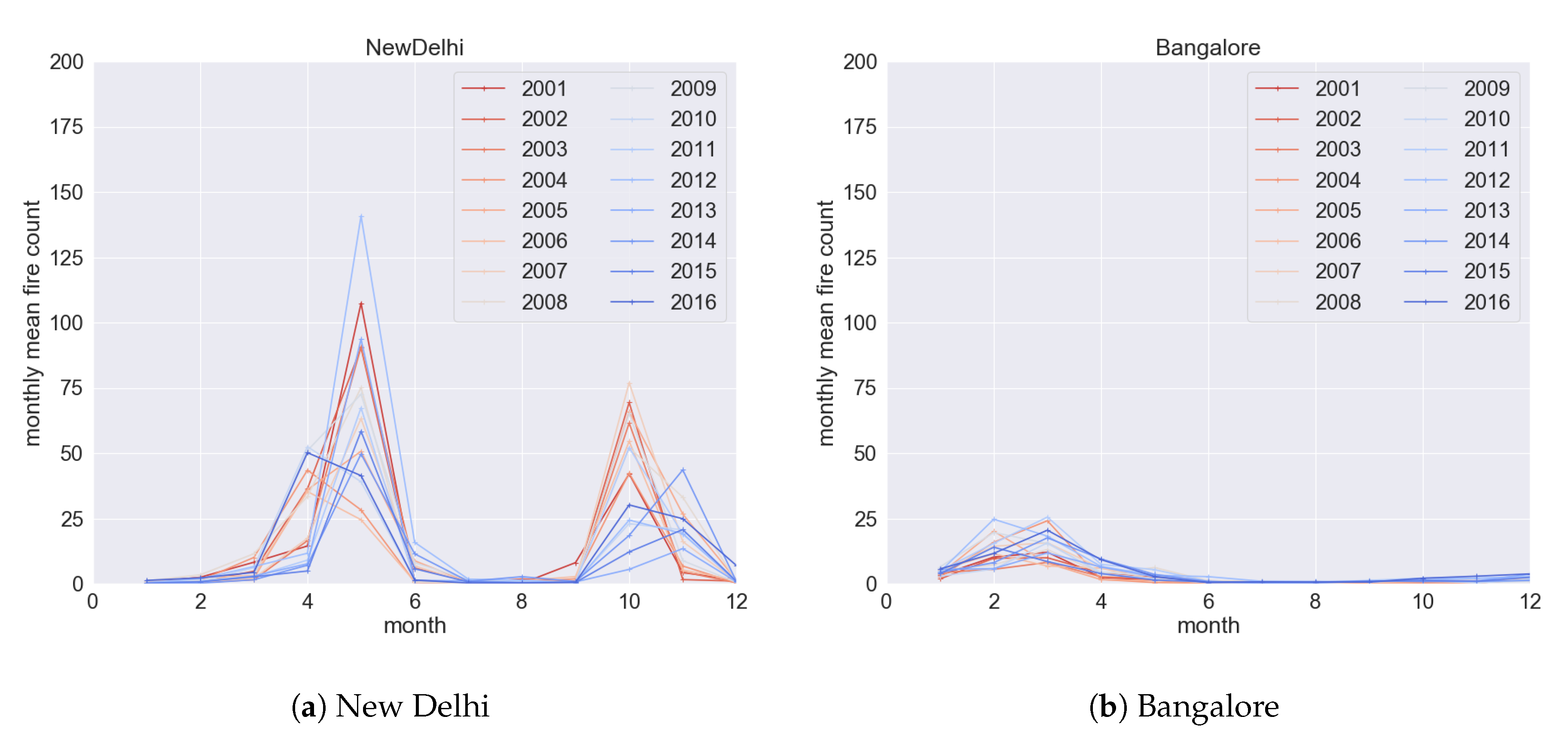
3.1.1. Seasonal Emission Activity Parameter

Most northern Indian cities (8 out of 9, except Jaipur) showed similar Pearson’s correlation values with respect to combination of s and r. Correlation between $R_{obs}$ and $R_{est}$ increased as $(s,r)$ values increased from (0.2, 0.2 ) to (0.7, 0.5). Another combination of $(s,r)$ values, around (0.1, 0.1), also showed higher correlation between $R_{obs}$ and $R_{est}$ but this was discarded on account of overfitting and insignificant model parameters (<90% confidence interval). On the basis of similar climate characteristics the same value of $(s,r)$, (0.6, 0.4) was used for all the cities in North India. In cities where summer and winter temperatures differ by less than <10 ${}^{\circ }$C, such as Chennai, Bangalore, Kolkata, Hyderabad and Mumbai, higher correlation coefficients between $R_{obs}$ and $R_{est}$ was obtained when the summer value s tended towards 1. This may indicate that summer and winter emissions are similar in location where strong temperature seasonality does not exist. For rainy season $SEA$ value r, the optimum values varied with the city’s location. Summary of the $(s,r)$ values chosen for each city is shown in

Table 3. Seasonal emission activity $SEA$ values by each city, used for summer s and rain r for residential ($A_R$) and commercial ($A_C$) emissions.

City	s	r
Chennai	0.7	0.6
Bangalore	0.9	0.9
Kolkata	0.8	0.8
Hyderabad	0.9	0.6
Mumbai	0.8	0.4
Ahmedabad	0.6	0.9
Jaipur	0.9	0.5
Others (North Indian city)	0.6	0.4

. Another set of $(s,r)$ was also investigated which was similar to those used in REASv2 emission inventory over India. The results obtained with those parameters are discussed in Tables S1 and S2 in Supplementary Materials.

3.1.2. Model Parameters

Emission coefficient parameter $EC$ for each $LU$ type as well the parameters for meteorological variables at city level and Tier level are shown in Figure 6. It is seen that model constant, $E{C}_O$ in Tier-2 cities (19.15 ± 3.92) is about 1.4 times that of Tier-1 cities (14.90 ± 4.79). Among residential, commercial and industrial regions, potency of concentrations due to emissions is highest for residential areas followed by industrial and commercial areas. $E{C}_R$ is higher for Tier-1 (0.001 ± 0.0004) than Tier-2 (0.0007 ± 0.0003), although when $E{C}_R$ of Jaipur and Ahmedabad is neglected, mean $E{C}_R$ of Tier-2 is higher than Tier-1. For some Tier-1 cities, like Hyderabad and Kolkata, $E{C}_I$ is higher than other cities suggesting industries in this locations are more polluting in nature compared to other Tier-1 cities. Contribution of a unit residential area (0.0006 ± 0.0002) is almost 1.5 times that of a unit industrial area (0.0004 ± 0.0003) in Tier-2 cities. Generally $E{C}_I$ had a higher coefficient of variation (ratio of mean and standard deviation) than $E{C}_R$ suggesting higher variation in industrial emitting sources. $E{C}_{BK}$ has the highest value among all the emission coefficient. $E{C}_{BK}$ is higher for Tier-1 (0.86 ± 0.31) than Tier-2 (0.53 ± 0.25). Out of the cities which have more brick kilns, some had much lower $E{C}_{B{K}_{m,s}}$, for example New Delhi. This could imply that the effect of an individual brick kiln on the urban R values is not significant in these cities compared to other emission sources. $E{C}_{agro}$ is higher in most cities compared to those cities where the problem of residue burning is not pervasive such as Hyderabad and Kolkata. However low $E{C}_{agro}$ for Ludhiana, which has the most crop residue fires is surprising and may imply that wind direction affects the impact of crop residue fires on the urban concentration. For a vehicle, its $E{C}_V$ is generally similar across the cities but overall it is higher in Tier-2 (8.47 × 10${}^{-9}$ ± 4.09 × 10${}^{-9}$) than Tier-1 (5.71 × 10${}^{-9}$ ± 4.21 × 10${}^{-9}$). This points the higher emission per vehicle in Tier-2 cities possibly as a result of vehicle age or emission regulations. Regarding coefficients for meteorological variables, the coefficient of planetary boundary layer height ${\beta }_{pblh}$ is negative and similar across the cities (−0.0008 ± 0.0005). The coefficient of wind, ${\beta }_{wnd}$ varies across the cities. It has a large absolute value in cities located in north-central Indo-Gangetic plain and those near the sea. ${\beta }_{wnd}$ is close to zero for New Delhi which implies a limited ability of the wind to flush out pollutants and lower the concentration. Given the skewness of ${\beta }_{wnd}$ towards zero for New Delhi, the wind maybe transporting PM${}_{2.5}$ due to emission from surrounding regions rather than help the city in lowering the concentrations. This is especially true during the crop residue burning months when winds assist long-range transport of aerosols from burning fields in the north-western India to New Delhi [82]. Coefficient for relative humidity, ${\beta }_{rh}$ is higher (0.31) in cities like Bangalore, Agra and Ludhiana which implies that aerosol composition has more hygroscopic aerosol in these cities than other cities (0.16).

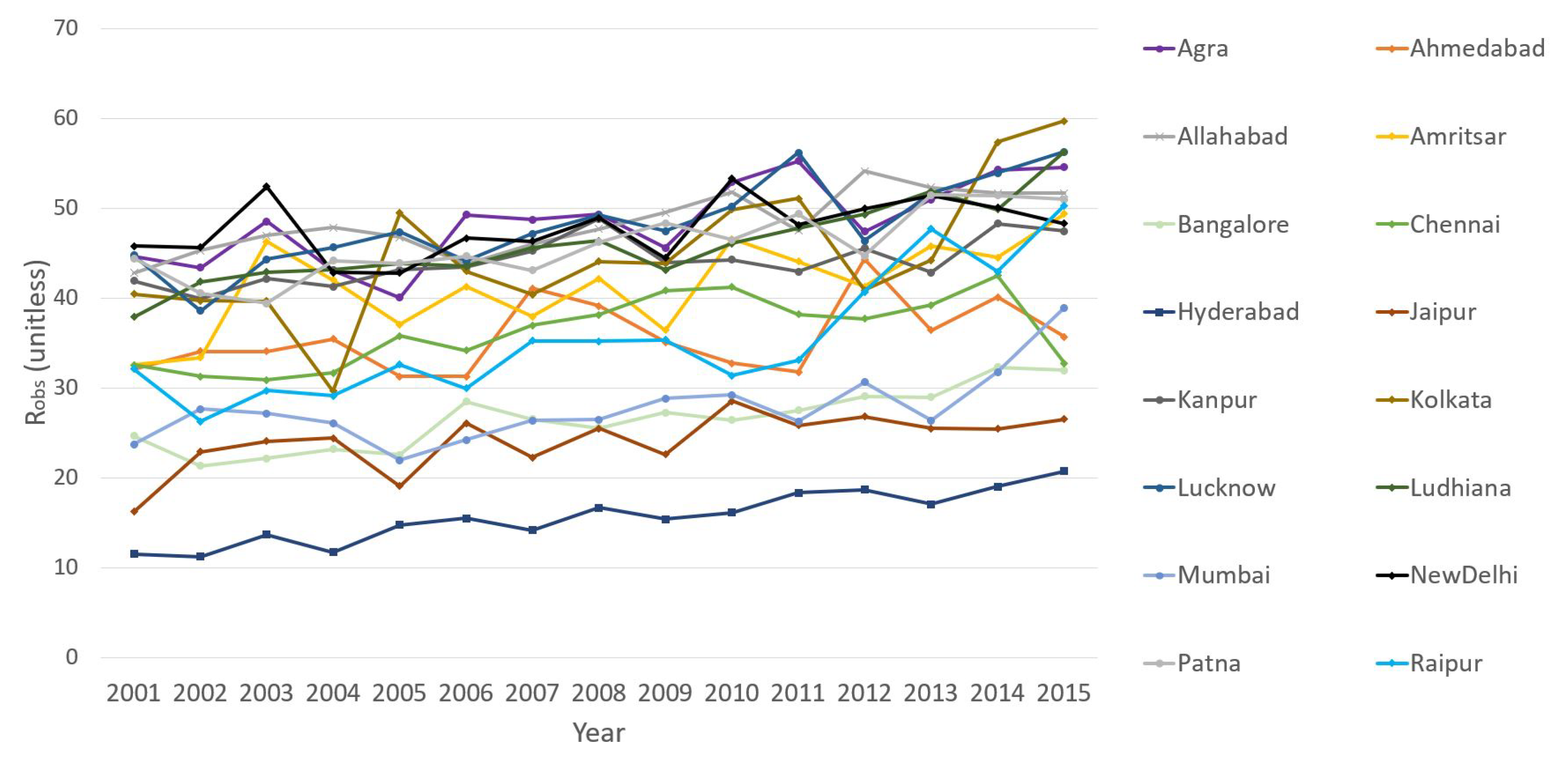
3.2. Long Term R Prediction and Out-of-Time Validation

The observed $R_{obs}$ and prediction of $R_{est}$ from the model trained on the 2001 and 2011 data is shown in Figure 7. The increasing trend in $R_{obs}$ is well predicted by $R_{est}$ and is on account of urban growth in residential, commercial, industrial ares and vehicle sectors. For some cases, the seasonality is also well captured in $R_{est}$ predictions. As the LUR model was trained only on 2001 and 2011 dataset, the confidence interval is large for those years whose $A_{LU}$ is quite different from that used for training. The overall Pearson’s correlations between out-of-time (excluding 2001 and 2011 dataset) $R_{obs}$ and $R_{est}$ is presented in

Table 4. Pearson’s correlation between $R_{obs}$ and $R_{est}$ for all years of the dataset 2001 to 2015. The significance was Bonferroni corrected to overcome multiple comparison problem. Significant correlations are den0ted by *.

Tier	City	Correlation	p-Value	95% Signficance
1	Chennai	0.62	0.0000	*
1	Mumbai	0.46	0.0000	*
1	NewDelhi	0.61	0.0000	*
1	Bangalore	0.43	0.0000	*
1	Hyderabad	0.35	0.0000	*
1	Kolkata	0.63	0.0000	*
2	Agra	0.46	0.0000	*
2	Ahmedabad	0.22	0.0032
2	Allahabad	0.66	0.0000	*
2	Kanpur	0.61	0.0000	*
2	Lucknow	0.52	0.0000	*
2	Ludhiana	0.28	0.0001	*
2	Patna	0.78	0.0000	*
2	Raipur	0.46	0.0000	*
2	Jaipur	−0.11	0.1480

, where the significance level was Bonferroni corrected to overcome multiple comparison problem. Jaipur and Ahmedabad have low and non-significant correlation. This could be a result of inappropriate $SEA$ which could not capture seasonal variation in emission behavior or the effect of meteorological dispersion is much stronger than local primary emissions. The rationale for suggesting this is that both Jaipur and Ahmedabad had quite different $SEA$ from the cities closest to them, New Delhi and Mumbai respectively. Both Jaipur and Ahmedabad are also on the edge of an arid desert region, where fine crustal particles may also play some role. However this needs further investigation. For other cities the correlation ranges from 0.28 to 0.78 (median correlation is 0.52). The correlation is high (>0.5) for cities already known to have high $R_{obs}$, e.g., Patna, Kolkata, New Delhi, Lucknow and Kanpur.

Accuracy of the monthly predictions $R_{est}$ was further explored by finding its root mean squared error (RMSE) with $R_{obs}$, as shown in Figure 8. The errors were not normally distributed throughout the months and were biased towards higher RMSE during the monsoon months of July, August and September for cities in northern India. RMSE in these cities during the monsoon months ranges from 12.9 to 23.9. During monsoon months R values are low not because the emissions are significantly low during this months, but rather there is a strong meteorological influence in the form of wet scavenging due to rain and wind. Also, due to cloudy sky very few retrievals can be made further reducing the validity of monthly mean of daily R values. There are also moderate RMSE values (mean 11.95) for the cooler months of December, January and February in many cities like New Delhi, Kanpur and Delhi. Due to cold weather and sunshine there is an enhanced formation of secondary particles that remain trapped as haze due to shallow boundary layer height. Lowest RMSE is obtained for the month of November (8.45) and April (9.69) suggesting the LUR predictions are most reliable in these months. Furthermore, for cities in Indo-Gangetic plains there is an underestimation in $R_{est}$ in October and December and overestimation in April and May. This is caused by the underestimation of fire counts in October by the MOD14 dataset and an increased secondary PM${}_{2.5}$ formation in December due to shallow boundary layer and stagnant winds.

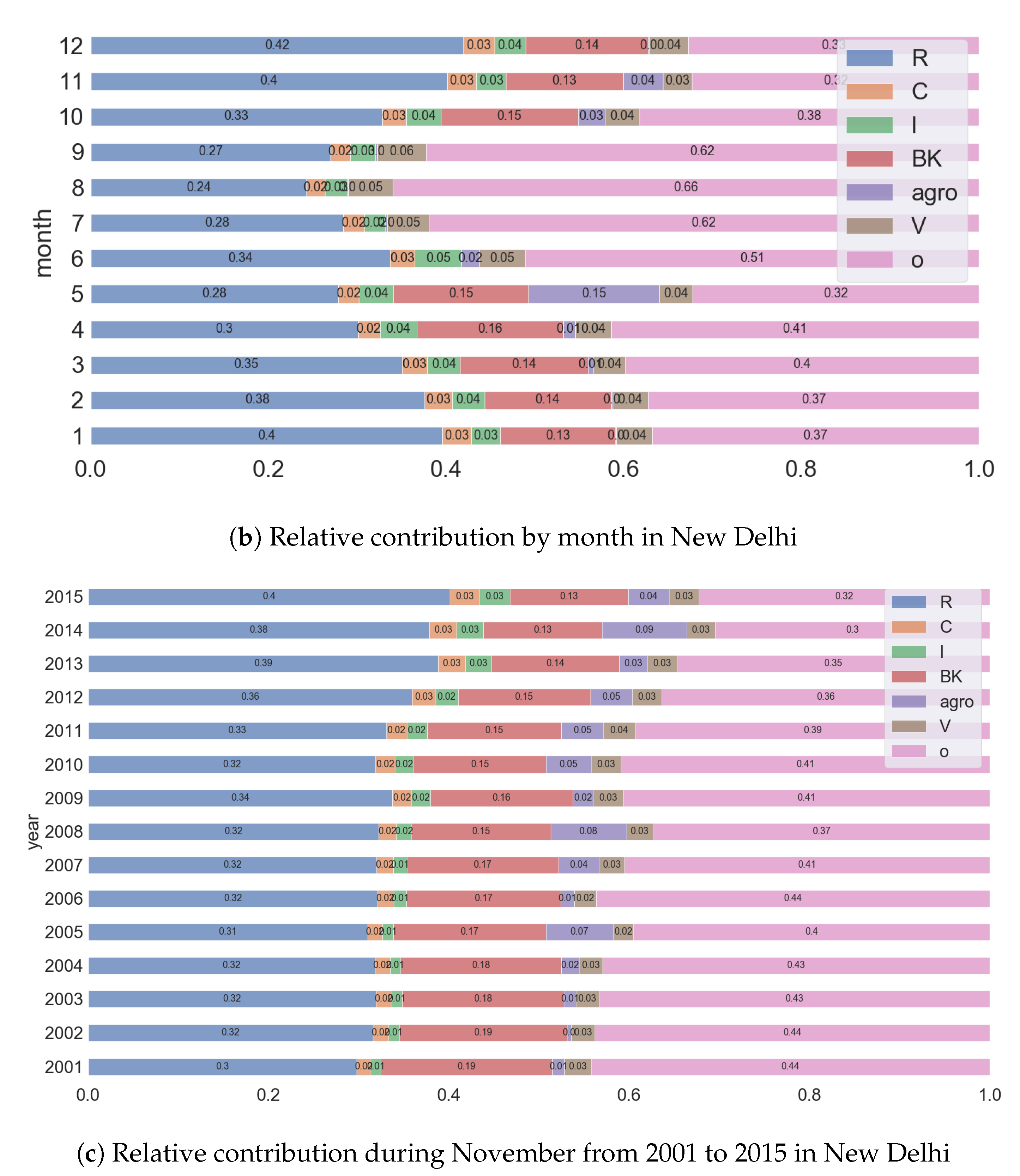
3.3. Source-Wise Relative Contribution

Relative contribution of $LU$ and other sources on the central 10 km × 10 km grid cell of cities and its seasonal variation is shown in Figure 9a and

Table 5. Comparison of relative contribution to $R_{est}$ over the central grid cell from concentration due to primary emission from $LU$ classes and other ($E{A}_O$) is presented for for all the cities for the year 2015 and month November. The contribution is represented by residential ($A_R$), commercial ($A_C$), industrial ($A_I$), agriculture related fires ($A_{agro}$), brick kilns ($A_{BK}$), vehicles ($A_V$). Contribution to $R_{est}$ due to formation of secondary particles, meteorological transport and unaccounted sources is collectively labeled as ‘others’.

City	${\mathit{A}}_{\mathit{R}}$	${\mathit{A}}_{\mathit{C}}$	${\mathit{A}}_{\mathit{I}}$	${\mathit{A}}_{\mathit{BK}}$	${\mathit{A}}_{\mathit{agro}}$	${\mathit{A}}_{\mathit{V}}$	Others
1 Chennai	38.7 ± 17.0	1.7 ± 1.4	3.8 ± 3.5	17.1 ± 8.9	0.0 ± 0.0	0.0 ± 0.0	38.6 ± 24.0
1 Mumbai	22.2 ± 15.4	14.1 ± 8.8	8.0 ± 5.4	0.0 ± 0.0	0.9 ± 0.3	2.1 ± 1.3	52.6 ± 11.9
1 NewDelhi	37.9 ± 10.3	3.0 ± 2.1	3.0 ± 1.9	13.1 ± 4.5	9.4 ± 2.2	3.1 ± 1.7	30.5 ± 6.9
1 Bangalore	15.6 ± 10.9	9.0 ± 6.2	1.8 ± 1.5	5.2 ± 4.2	0.3 ± 0.1	3.7 ± 2.3	64.3 ± 22.9
1 Hyderabad	14.2 ± 13.1	13.7 ± 10	27.7 ± 15.3	0.0 ± 0.0	0.4 ± 0.3	19.7 ± 13.8	24.3 ± 22.5
1 Kolkata	39.3 ± 16.0	2.2 ± 1.8	9.7 ± 5.4	25.3 ± 7.3	0.2 ± 0.1	1.0 ± 0.9	22.2 ± 10.9
1 Agra	59.1 ± 13.1	0.5 ± 0.4	2.6 ± 1.4	3.2 ± 1.9	1.2 ± 0.8	0.1 ± 0.1	33.3 ± 13.2
2 Ahmedabad	6.8 ± 5.7	2.0 ± 1.4	7.8 ± 4.7	4.0 ± 3.8	0.7 ± 0.3	0.5 ± 0.3	78.2 ± 12.7
2 Allahabad	65.1 ± 13.5	0.1 ± 0.1	1.0 ± 0.9	6.6 ± 4.4	0.4 ± 0.2	0.0 ± 0.0	26.8 ± 10.6
2 Kanpur	43.3 ± 11.0	0.3 ± 0.3	1.7 ± 1.3	14.4 ± 6.0	0.7 ± 0.3	0.2 ± 0.2	39.3 ± 11.1
2 Lucknow	49.2 ± 8.3	0.6 ± 0.5	0.7 ± 0.6	10.6 ± 5.4	0.5 ± 0.2	0.7 ± 0.5	37.7 ± 11.9
2 Ludhiana	42.3 ± 12.0	0.2 ± 0.2	3.4 ± 1.9	3.6 ± 3.1	4.4 ± 2.3	0.1 ± 0.1	45.9 ± 10.9
2 Patna	56.3 ± 11.5	0.5 ± 0.4	6.7 ± 3.6	21.6 ± 5.2	0.2 ± 0.1	0.0 ± 0.0	14.7 ± 8.8
2 Raipur	22.5 ± 10.6	0.2 ± 0.2	1.7 ± 1.6	8.7 ± 5.5	1.1 ± 0.3	0.1 ± 0.0	65.7 ± 13.8
2 Jaipur	11.9 ± 10.7	3.3 ± 2.8	6.4 ± 5.9	5.0 ± 4.6	5.7 ± 2.5	0.2 ± 0.1	67.5 ± 19.8

. Since the RMSE between $R_{est}$ and $R_{obs}$ was lowest for November (discussed in previous section), the relative contributions are discussed based on the result for this month. Residential areas have the highest contribution due to primary emission than other $LU$ classes. Contribution of residential areas is higher in Tier-2 cities (39.6 ± 10.7%) than Tier-1 cities (28.0 ± 13.8%). This could be due poor enforcement of regulations regarding waste combustion, fine-dust from construction and road as well as burning biomass for fuel. If brick kilns are present, then they have the highest contribution (11.7 ± 5.2%) after residential areas. Their contribution is higher in Tier-1 cities as those cities are rapidly undergoing urban expansion and require construction materials. Contribution of commercial (7.3 ± 5.1%) and industrial (9.0 ± 5.5%) areas in Tier-1 cities is higher than the contribution of commercial (0.9 ± 0.7%) and industrial (3.6 ± 2.4%) areas in Tier-2 cities. Underestimation of the total areas under industries could have led to lower contribution of industrial sources than what is reported elsewhere. Contribution of vehicles to concentration is also quite low and observed only for the Tier1 cities. Hyderabad has a higher vehicle contribution, however this is on account of the very high vehicle population. It is also possible that spatial variation in concentration due to emission from industrial point sources and road network is not captured distinctly within the 10 km resolution of R pixels. Availability of retrievals at higher resolution from satellite such as Sentinel-5P [83] may overcome this limitation. Crop fires contribute negligibly to $R_{est}$ in most cities except New Delhi (9.4 ± 2.2%) and Ludhiana (4.4 ± 2.3%) which are in close proximity to such farm fields. This post-monsoon agricultural fire contribution is likely an underestimation due to the known issue of low fire counts reported in MOD14 product during post-monsoon season [60].

A significant portion of relative contributions is accorded to other sources and secondary aerosol formation as seen by a large estimation of $E{A}_O$ in Tier-1 cities (38.8 ± 16.5%) as well as Tier-2 cities (45.5 ± 12.5%). High contribution $E{A}_O$ to R could be on account of secondary PM${}_{2.5}$ formation which is a result of aerosol chemistry and meteorology. During high pollution episodes, the relative contribution of secondary PM${}_{2.5}$ is high [84,85]. Stagnant meteorology, for example, low wind speed, high humidity and shallow boundary layer, also enhance secondary PM${}_{2.5}$ formation [84]. This includes complicated transformation pathways like oxidation of precursor gases like SO${}_2$, NO${}_x$ and NH${}_3$ to aerosols, that cannot be resolved with our data-based approach which relies on statistically linking emissions with concentrations. Some cities also have a high contribution of $E{A}_O$ due to proximity to sources like power and steel plants as well coal mines. Using bottom-up emission inventories, Guttikunda et al. [86] recently concluded that the meteorological transport of pollutants from surrounding peri-urban and rural areas in many cities makes it difficult to segregate contributions based on the to urban PM${}_{2.5}$ alone. They also found that outside contribution is higher in Tier-2 cities and ranges between 30% to 40%. In Figure 9, overall emissions from residential areas contributed the most to R in urban areas (35.0 ± 11.9%), followed by brick kilns (11.7 ± 5.2%) and industries (4.2 ± 2.8%) over central part. The contribution of other sources is around 41.6% in Tier-1 and 45.5% in Tier-2 cities.

For monthly changes in relative contributions, an example for New Delhi for the year 2015 is presented in Figure 9b. Monthly changes in relative contributions are regulated by the $SEA$ parameter, agricultural fire counts and meteorology. It is seen that contribution of agricultural fire is highest during May, October and November. Checking relative contributions for the month of November across the years shows that contribution of agricultural fires has increased from the 2001–2005 period (2.5%) to the 2010–2015 period (5.2%). This is due to recent groundwater related policy that suggests delay in sowing of the crop [87]. It is also seen that contribution of residential areas has increased from 2001 (29.7 ± 8.0%) to 2015 (40.0 ± 10.9%). Since we assumed a constant count of brick kilns for all the years it appears that the contribution of brick kilns is decreasing from 19.0% to 13.1% which may be incorrect. Nonetheless it does suggest that brick kiln as a significant contributor to $R_{est}$ values in New Delhi. Based on the decrease in contribution of $E{A}_O$ from 2001 to 2015, it can be said that contribution can be explained more by the sources within the city in recent years.

Comparison with Other Studies

The relative contribution results from our LUR based approach were also compared with those from some recent studies. There have been dispersion modeling (DM), source apportionment (SA), bottom-up emission inventory (EI), receptor modeling (RM) based studies in Indian cities to identify the contribution of the emitters to the urban PM${}_{2.5}$ concentration. On an overall country-wide scale Venkataraman et al. [88] have stated that about 60% of India’s mean population-weighted PM${}_{2.5}$ concentrations come from anthropogenic source sectors, like residential biomass combustion, industrial coal combustion, while the remainder are from ‘other’ sources, like transportation, brick production, windblown dust and extra-regional sources. Secondary PM${}_{2.5}$ is known to contribute upto 42 ± 10% in winter and 23 ± 6% in summer [89]. Along with fine dust, contribution of secondary particles can rise upto 52% in winter and 65% in summer [89]. Recent research by Guo et al. [90] over few Indian cities also found that residential sources are dominant contributor to primary particulate matter; contributing 67% and 44% in Lucknow and New Delhi respectively. In comparison, our estimate of residential contribution to concentration due to primary emissions is 78.9 ± 8.3% and 54.5 ± 10.3%. Resulting concentration from primary emissions was also compared with PM${}_{2.5}$ emissions from REASv2 inventory for New Delhi. Among urban emitters, REASv2 distinguishes PM${}_{2.5}$ emissions between domestic, industrial and vehicles. Therefore relative contribution of these REASv2 based emissions was compared with our model’s residential, total industrial and brick kiln emissions and vehicle emissions. When trends were compared for any particular month across 8 years, the correlation was quite high (>0.9). An example for the month of January is shown in Figure 10. Summary of contribution from other studies is shown in

Table 6. Summary of recent source contribution studies (in percentage) by emission mass contribution or concentration contribution using dispersion modeling (DM), source apportionment (SA), bottom-up emission inventory (EI), receptor modeling (RM) methods are shown here. The sectors residential (R), commercial (C), industrial (I), biomass burning (agro), brick kiln (BK), vehicles (V), construction dust (dust), other non-accounted sources (other), secondary particles (Sec.) and power plants (PP). Summer and winter time contribution are denoted by S and W.

Ref.	City	Year	Method	R	C	I	Agro	BK	V	Dust	Other	Sec.	PP
[92]	Chennai	2010	DM		8				27	24		13	26
[86]	Chennai	2015	SA	18	2	13		3	25	24	15
[91]	Delhi(S)	2016	RM			11	15		18	34	5	17
[91]	Delhi(W)	2016	RM			10	22		23	15	4	26
[91]	Delhi(S)	2016	DM	8		22	7		17	38	8
[91]	Delhi(W)	2016	DM	10		30	4		28	17	11
[32]	Delhi	2010	EI	20	6	14		15	17	11			16
[92]	Delhi	2010	SA	67		3	3		22	5
[30]	Delhi	2010	EI	27		24			45				4
[92]	Bangalore	2010	SA	6	28				47	4		13
[86]	Bangalore	2015	DM	26	4	2		2	27	23	16
[93]	Hyderabad	2010	SA	15		7			31	26	21
[86]	Agra	2015	DM	36	3	0		0	14	10	36
[94]	Kanpur	2011	EI	24	4	26	4		20	14	8
[92]	Kanpur	2010	SA	27	17	2			23	5		25
[86]	Kanpur	2015	DM	42	4	7		1	13	9	22
[86]	Ludhiana	2015	DM	17	3	8		3	16	12	40
[86]	Patna	2015	DM	27	5	11		10	15	12	19
[86]	Raipur	2015	DM	18	3	23		2	17	12	26

. Several studies have reported construction dust separately from residential emissions. Since our model does not identify construction dust separately we combined this with residential when making comparisons. For New Delhi residential contributions others have estimated 34% [91], 46% [91], 27% [91] and 31% [32] which is similar to our estimate of 37.9 ± 10.3%. Our estimates of contribution of $E{A}_O$ is 30.5 ± 6.9 similar to 30% by ARAI and TERI [91]. Guttikunda and Calori [32] also found contribution of brick kilns to be 15% similar to 13.1 ± 4.5% by us. For agricultural fires the estimate of 4% [91] is near to 9.4 ± 2.2% by us. Our estimates for Chennai are close with both [92] and [86] when accounting for the uncertainties. Contribution of residential and others by Central Pollution Control Board [92] was 24% and 39% and by Guttikunda et al. [86] was 42% and 15% compared to 38.7 ± 17.0% and 38.6 ± 24.0% by our estimate in Chennai. For Kanpur, Guttikunda et al. [86] estimated contribution of residential areas and others as 42% and 22% similar to 43.3 ± 11.0% and 39.3 ± 11.1 by us. For Raipur, Guttikunda et al. [86] estimated contribution of residential areas and brick kilns as 18% and 3% compared to 22.5 ± 10.6 and 8.7 ± 5.5%. The definition of the emitting sources has varied from study to study when the researchers have created their own emission inventory or method and this study is no exception. This presents challenges in comparing our results to other studies using well-established methods. It appears our estimates of contribution are mostly consistent for residential areas and there is slight agreement for brick kilns and agricultural fire contributions.

3.4. Limitations

The model relies on $SEA$ for estimating seasonal variation in $R_{em}$. As only that set of $SEA$ were chosen that maximize correlation between $R_{obs}$ and $R_{est}$, endogeneity may be induced in the model. However currently there is no approach to estimate $SEA$ using open gridded datasets. Monthly changes in the nighttime light datasets could inform variation in intensity of human-level emission activities [95,96]. The relative contributions estimated (Section 3.3) by our approach correspond to contribution to concentration due to primary emission of PM${}_{2.5}$. Although this is a limitation during the months of high PM${}_{2.5}$ concentration when the total concentration is being regulated by secondary PM${}_{2.5}$ formation, framing control policies for primary emission is easier than secondary formation and control of primary emission may also offer co-benefits in reducing precursor gases [94].

The accuracy of the relative contributions calculated by our approach is limited by the statistical approach as well as datasets that were used. In the LUR model as precursor gas emissions were not explicitly considered, secondary PM${}_{2.5}$ formation is not accounted for the model. So at high R values, our model’s prediction accuracy diminishes. This is especially true for the month of December in northern Indian cities when $R_{est}$ predictions are lower than the $R_{obs}$ as the $R_{obs}$ is being contributed by secondary formation. Also a linear dependence is assumed between R and independent variables [5,21]. Yet complex chemical and physical interactions between the variables may take place that cannot be resolved by LUR, as others have pointed out. A common situation is that high summer atmospheric temperatures enhances formation secondary PM${}_{2.5}$ while leading to an elevated boundary layer height that increases dispersion of PM${}_{2.5}$. Further research is needed over whether a combination of land use regression model and chemical transport model would work as well over the highly polluted Indian cities as the performance over West Europe [97] and United States [98]. Regarding the data that was used for training the LUR model, uncertainties are present in R as well as land-use area estimations. R has an uncertainty of about ±16, which is lower than the range of monthly mean values R but not reliable when investigating smaller R variations at daily scale or months with similar meteorological conditions. The impact of missing observations during the cloudy months lead to a high RMSE, thus affecting the prediction accuracy. Impact of the missing observations was further explored in Table S3 of Supplementary Materials and suggests that better interpolation techniques may be useful. At the same time, accuracy of land-use classifications obtained for residential, commercial and industrial areas is not consistent across the cities, varying between 64% and 95% and being low especially for identification for industrial areas. This could have led to the identification of relative contribution of industrial emission being lower compared to other researches. Due to availability of spatial training data for only 2001 and 2011, the models implicitly assumes linear urban growth. However non-uniform annual urban land-use expansion could take place in the intervening years under influence of population growth and per capita GDP growth. This is briefly explored in Table S4 of Supplementary Materials and suggests there may be slight variation in the contributions. Furthermore, it was assumed that all members belonging to an emitting sector have similar emission characteristics. This may be true for residential and commercial areas to some extent but industrial emissions vary greatly among themselves. For example, certain industrial structures that are involved as warehousing do not cause significant emissions. Further research must be taken to categorically differentiate high polluting industries from the low polluting industries on the basis of chimney size [99] or other characteristics. We used approximate counts of brick kilns based on visual interpretation. Work is under progress to prepare a brick kiln location dataset that can be used in LUR and CTM models. Fire counts obtained from the MOD14 based product are also known to underestimate counts during the crop residue burning due to a combination of crop residue characteristics, burning time and fire intensity. Recently launched VIIRS based fire count has been shown to overcome this issue to a large extent and further research is needed to improve retrospective MOD14 fire counts by using VIIRS based product.

3.5. Policy Implications

Implications for policy can be derived based on results regarding relative contribution of each $LU$ type in Tier-1 and Tier-2. In India, most discussion of air quality policies is focused around Tier-1 cities [86]. However anthropogenic fine particle concentration is rising in other cities as well. Thus, Central Pollution Control Board of India may need emission policies in Tier-1 and Tier-2 based on separate priorities as the composition of relative contributions is different. Furthermore, current policies are biased towards regulating emission factors for vehicles, when it should also consider the vehicle kilometer traveled due to urban expansion, for example, we found a negative correlation of vehicle kilometer traveled with built-up density and largest patch index. With tighter vehicle emission norms and announcement of 30% ‘electric vehicle policy’ by 2030 in India [100], their relative contribution may reduce in the future. Emissions from residential areas must be investigated and regulated strictly as they have the maximum contribution to R in the urban areas. Recent attention has revealed the strongly adverse impact of open waste burning, construction, road-dust, traditional cooking methods and so forth, from residential areas. As these emissions are related to socioeconomic development in the form of urban expansion, policy is needed to expedite technological evolution such that PM${}_{2.5}$ emissions may be decoupled from urban expansion. Since the model presented in this paper identifies emissions from per unit area of land-use class, it provides an approach for desired technological improvement to ensure required particulate emission. Brick kilns also contribute heavily to R, which implies implementation failure of current policy in ensuring their upgradation. Constructions technologies that reduces reliance on polluting brick kilns must also be explored. This is especially important for cities that have a large area and are expected to see more urbanization.

4. Conclusions

The goal of this research was to estimate the impact on long-term (2001 to 2015) PM${}_{2.5}$ concentrations due to urban growth in 15 Indian cities with land-use regression model using remote sensing and meteorological datasets. The specific objective was to calculate relative contribution of the land-use and vehicular sources to urban fine aerosol concentration and compare the results with non-remote sensing based estimations. Ambient PM${}_{2.5}$ concentration from 2001 to 2015 was indicated by a MODIS based product called R, created in a previous research. The experimental setup was modeled as a land use regression model with inverse distance weighting in a hierarchical Bayesian framework with Tier of a city as random effect. Land-use emission sources considered were residential, commercial and industrial units, agricultural crop fires and brick kilns. Land use regression could successfully predict rising R due to urban growth showing a correlation higher than 0.5 in 7 out of the 15 cities considered. We provide evidence that above the central portion of a city, concentration due to primary PM${}_{2.5}$ emission is contributed mostly by residential areas (35.0 ± 11.9%), brick kilns (11.7 ± 5.2%) and industries (4.2 ± 2.8%). However their contribution differed between Tier-1 and Tier-2 cities which implies current policies must consider a city’s socioeconomic growth status while designing policy measures. Scattered urban form of Tier-1 cities may cause high vehicle kilometers traveled leading to higher vehicular contribution in Tier-1. Parameters of annual seasonal emission activity and underestimation in MODIS fire count affected correlation with long-term trend. Trend of monthly comparison of R value estimated by the model showed high correlation with REASv2 PM${}_{2.5}$ emissions (∼0.9). Comparisons with recent researches confirmed similarity of contribution estimated from residential areas and to some extent from brick kilns and agricultural fires. Upto 42.8 ± 14.1% contribution is attributed to formation of secondary aerosol, long-range transport and unaccounted sources in surrounding regions especially for Tier-2 cities. This is similar to findings from some recent studies. Due to their high contribution, it is suggested that policymakers must consider regulations for emissions from residential areas and brick kilns.

References

1. Van Donkelaar, A.; Martin, R.V.; Park, R.J. Estimating ground-level PM2.5 using aerosol optical depth determined from satellite remote sensing. J. Geophys. Res. Atmos. 2006, 111, 1–10. [Google Scholar] [CrossRef]
2. Itahashi, S.; Uno, I.; Yumimoto, K.; Irie, H.; Osada, K.; Ogata, K.; Fukushima, H.; Wang, Z.; Ohara, T. Interannual variation in the fine-mode MODIS aerosol optical depth and its relationship to the changes in sulfur dioxide emissions in China between 2000 and 2010. Atmos. Chem. Phys. 2012, 12, 2631–2640. [Google Scholar] [CrossRef] [Green Version]
3. Akimoto, H.; Ohara, T.; Kurokawa, J.I.; Horii, N. Verification of energy consumption in China during 1996–2003 by using satellite observational data. Atmos. Environ. 2006, 40, 7663–7667. [Google Scholar] [CrossRef]
4. De Meij, A.; Krol, M.; Dentener, F.; Vignati, E.; Cuvelier, C.; Thunis, P. The sensitivity of aerosol in Europe to two different emission inventories and temporal distribution of emissions. Atmos. Chem. Phys. Discuss. 2006, 6, 3265–3319. [Google Scholar] [CrossRef] [Green Version]
5. Zou, B.; Chen, J.; Zhai, L.; Fang, X.; Zheng, Z. Satellite based mapping of ground PM2.5 concentration using generalized additive modeling. Remote Sens. 2017, 9, 1. [Google Scholar] [CrossRef]
6. Reyes, J.M.; Serre, M.L. An LUR/BME framework to estimate PM2.5 explained by on road mobile and stationary sources. Environ. Sci. Technol. 2014, 48, 1736–1744. [Google Scholar] [CrossRef] [PubMed]
7. Briggs, D.J.; Collins, S.; Elliott, P.; Fischer, P.; Kingham, S.; Lebret, E.; Pryl, K.; Van Reeuwijk, H.; Smallbone, K.; Van Der Veen, A. Mapping urban air pollution using gis: A regression-based approach. Int. J. Geogr. Inf. Sci. 1997, 11, 699–718. [Google Scholar] [CrossRef]
8. Briggs, D.J.; de Hoogh, C.; Gulliver, J.; Wills, J.; Elliotta, P.; Kinghamc, S.; Smallboned, K. A regression-based method for mapping traffic-related air pollution:application and testing in four contrasting urban environments. Sci. Total Environ. 2000, 253, 151–167. [Google Scholar] [CrossRef]
9. Hankey, S.; Marshall, J.D. Land Use Regression Models of On-Road Particulate Air Pollution (Particle Number, Black Carbon, PM2.5, Particle Size) Using Mobile Monitoring. Environ. Sci. Technol. 2015, 49, 9194–9202. [Google Scholar] [CrossRef]
10. Lin, G.; Fu, J.; Jiang, D.; Hu, W.; Dong, D.; Huang, Y.; Zhao, M. Spatio-temporal variation of PM2.5 concentrations and their relationship with geographic and socioeconomic factors in China. Int. J. Environ. Res. Public Health 2014, 11, 173–186. [Google Scholar] [CrossRef]
11. Gong, J.; Hu, Y.; Liu, M.; Bu, R.; Chang, Y.; Bilal, M.; Li, C.; Wu, W.; Ren, B. Land Use Regression Models Using Satellite Aerosol Optical Depth Observations and 3D Building Data from the Central Cities of Liaoning Province, China. Polish J. Environ. Stud. 2016, 25, 1015–1026. [Google Scholar] [CrossRef]
12. Zhou, C.; Chen, J.; Wang, S. Examining the effects of socioeconomic development on fine particulate matter (PM 2.5) in China’s cities using spatial regression and the geographical detector technique. Sci. Total Environ. 2018, 619–620, 436–445. [Google Scholar] [CrossRef] [PubMed]
13. Naughton, O.; Donnelly, A.; Nolan, P.; Pilla, F.; Misstear, B.D.; Broderick, B. A land use regression model for explaining spatial variation in air pollution levels using a wind sector based approach. Sci. Total Environ. 2018, 630, 1324–1334. [Google Scholar] [CrossRef] [PubMed] [Green Version]
14. Brauer, M.; Freedman, G.; Frostad, J.; van Donkelaar, A.; Martin, R.V.; Dentener, F.; Van Dingenen, R.; Estep, K.; Amini, H.; Apte, J.S.; et al. Ambient Air Pollution Exposure Estimation for the Global Burden of Disease 2013. Environ. Sci. Technol. 2016, 79–88. [Google Scholar] [CrossRef] [PubMed]
15. Misra, P.; Fujikawa, A.; Takeuchi, W. Novel decomposition scheme for characterizing urban air quality with MODIS. Remote Sens. 2017, 9, 812. [Google Scholar] [CrossRef]
16. Van Donkelaar, A.; Martin, R.V.; Brauer, M.; Hsu, N.C.; Kahn, R.A.; Levy, R.C.; Lyapustin, A.; Sayer, A.M.; Winker, D.M. Global Estimates of Fine Particulate Matter using a Combined Geophysical-Statistical Method with Information from Satellites, Models, and Monitors. Environ. Sci. Technol. 2016, 50, 3762–3772. [Google Scholar] [CrossRef] [PubMed]
17. Beelen, R.; Voogt, M.; Duyzer, J.; Zandveld, P.; Hoek, G. Comparison of the performances of land use regression modelling and dispersion modelling in estimating small-scale variations in long-term air pollution concentrations in a Dutch urban area. Atmos. Environ. 2010, 44, 4614–4621. [Google Scholar] [CrossRef]
18. Johnson, M.; Isakov, V.; Touma, J.S.; Mukerjee, S.; Özkaynak, H. Evaluation of land-use regression models used to predict air quality concentrations in an urban area. Atmos. Environ. 2010, 44, 3660–3668. [Google Scholar] [CrossRef]
19. Saraswat, A.; Apte, J.S.; Kandlikar, M.; Brauer, M.; Henderson, S.B.; Marshall, J.D. Spatiotemporal land use regression models of fine, ultrafine, and black carbon particulate matter in New Delhi, India. Environ. Sci. Technol. 2013, 47, 12903–12911. [Google Scholar] [CrossRef]
20. Sanchez, M.; Ambros, A.; Milà, C.; Salmon, M.; Balakrishnan, K.; Sambandam, S.; Sreekanth, V.; Marshall, J.D.; Tonne, C. Development of land-use regression models for fine particles and black carbon in peri-urban South India. Sci. Total Environ. 2018, 634, 77–86. [Google Scholar] [CrossRef]
21. Upadhyay, A.; Dey, S.; Goyal, P.; Dash, S.K. Projection of near-future anthropogenic PM2.5 over India using statistical approach. Atmos. Environ. 2018, 186, 178–188. [Google Scholar] [CrossRef]
22. World Health Organization. WHO Global Ambient Air Quality Database (Update 2018); World Health Organization: Geneva, Switzerland, 2018. [Google Scholar]
23. Kaya, Y. Impact of Carbon Dioxide Emission Control on GNP Growth: Interpretation of Proposed Scenarios; IPCC Energy and Industry Subgroup, Response Strategies Working Group: Paris, France, 1989. [Google Scholar]
24. IPCC. Climate Change 2014: Mitigation of Climate Change. Working Group III Contribution to the Fifth Assessment Report of the Intergovernmental Panel on Climate Change; Cambridge University Press: Cambridge, UK; New York, NY, USA, 2014. [Google Scholar]
25. Ohara, T.; Akimoto, H.; Kurokawa, J.; Horii, N.; Yamaji, K.; Yan, X.; Hayasaka, T. An Asian emission inventory of anthropogenic emission sources for the period 1980–2020. Atmos. Chem. Phys. 2007, 7, 4419–4444. [Google Scholar] [CrossRef]
26. Kurokawa, J.; Ohara, T.; Morikawa, T.; Hanayama, S.; Janssens-Maenhout, G.; Fukui, T.; Kawashima, K.; Akimoto, H. Emissions of air pollutants and greenhouse gases over Asian regions during 2000–2008: Regional Emission inventory in ASia (REAS) version 2. Atmos. Chem. Phys. 2013, 13, 11019–11058. [Google Scholar] [CrossRef]
27. Reddy, M.; Venkataraman, C. Inventory of aerosol and sulphur dioxide emissions from India: I—Fossil fuel combustion. Atmos. Environ. 2002, 36, 677–697. [Google Scholar] [CrossRef]
28. Sadavarte, P.; Venkataraman, C. Trends in multi-pollutant emissions from a technology-linked inventory for India: I. Industry and transport sectors. Atmos. Environ. 2014, 99, 353–364. [Google Scholar] [CrossRef]
29. Bhanarkar, A.D.; Rao, P.S.; Gajghate, D.G.; Nema, P. Inventory of SO2, PM and toxic metals emissions from industrial sources in Greater Mumbai, India. Atmos. Environ. 2005, 39, 3851–3864. [Google Scholar] [CrossRef]
30. Sahu, S.K.; Beig, G.; Parkhi, N.S. Emissions inventory of anthropogenic PM2.5 and PM10 in Delhi during Commonwealth Games 2010. Atmos. Environ. 2011, 45, 6180–6190. [Google Scholar] [CrossRef]
31. Baidya, S.; Borken-Kleefeld, J. Atmospheric emissions from road transportation in India. Energy Policy 2009, 37, 3812–3822. [Google Scholar] [CrossRef] [Green Version]
32. Guttikunda, S.K.; Calori, G. A GIS based emissions inventory at 1 km × 1 km spatial resolution for air pollution analysis in Delhi, India. Atmos. Environ. 2013, 67, 101–111. [Google Scholar] [CrossRef]
33. Paliwal, U.; Sharma, M.; Burkhart, J.F. Monthly and spatially resolved black carbon emission inventory of India: Uncertainty analysis. Atmos. Chem. Phys. 2016, 16, 12457–12476. [Google Scholar] [CrossRef]
34. Maithel, S.; Uma, R.; Bond, T.; Baum, E.; Thao, V. Brick Kilns Performance Assessment A Roadmap for Cleaner Brick Production in India; Technical Report April; Greentech Knowledge Solutions: New Delhi, India, 2012. [Google Scholar]
35. Venkataraman, C.; Habib, G.; Kadamba, D.; Shrivastava, M.; Leon, J.F.; Crouzille, B.; Boucher, O.; Streets, D.G. Emissions from open biomass burning in India: Integrating the inventory approach with high-resolution Moderate Resolution Imaging Spectroradiometer (MODIS) active-fire and land cover data. Glob. Biogeochem. Cycles 2006, 20, 1–12. [Google Scholar] [CrossRef]
36. Rosa, E.A.; Dietz, T. Human drivers of national greenhouse-gas emissions. Nat. Clim. Change 2012, 2, 581–586. [Google Scholar] [CrossRef]
37. Chertow, M.R. The IPAT Equation and Its Variants. J. Industrial Ecol. 2000, 4, 13–29. [Google Scholar] [CrossRef]
38. Sun, J.W. The decrease of CO2 emission intensity is decarbonization at national and global levels. Energy Policy 2005, 33, 975–978. [Google Scholar] [CrossRef]
39. Wang, J. Intercomparison between satellite-derived aerosol optical thickness and PM 2.5 mass: Implications for air quality studies. Geophys. Res. Lett. 2003, 30, 2095. [Google Scholar] [CrossRef]
40. Gupta, P.; Christopher, S.A. Particulate matter air quality assessment using integrated surface, satellite, and meteorological products: Multiple regression approach. J. Geophys. Res. Atmos. 2009, 114, 1–13. [Google Scholar] [CrossRef]
41. Levy, R.C.; Remer, L.A.; Kleidman, R.G.; Mattoo, S.; Ichoku, C.; Kahn, R.; Eck, T.F. Global evaluation of the Collection 5 MODIS dark-target aerosol products over land. Atmos. Chem. Phys. 2010, 10, 10399–10420. [Google Scholar] [CrossRef] [Green Version]
42. Li, J.; Jin, M.; Xu, Z. Spatiotemporal variability of remotely sensed PM2.5 concentrations in China from 1998 to 2014 based on a bayesian hierarchy model. Int. J. Environ. Res. Public Health 2016, 13, 772. [Google Scholar] [CrossRef] [PubMed]
43. Roy, D.P.; Lewis, P.; Schaaf, C.B.; Devadiga, S.; Boschetti, L. The global impact of clouds on the production of MODIS bidirectional reflectance model-based composites for terrestrial monitoring. IEEE Geosci. Remote Sens. Lett. 2006, 3, 452–456. [Google Scholar] [CrossRef]
44. Levy, R.; Leptoukh, G.; Kahn, R.; Zubko, V.; Gopalan, A.; Remer, L. A Critical Look at Deriving Monthly Aerosol Optical Depth From Satellite Data. IEEE Trans. Geosci. Remote Sens. 2009, 47, 2942–2956. [Google Scholar] [CrossRef]
45. Christopher, S.A.; Gupta, P. Satellite Remote Sensing of Particulate Matter Air Quality: The Cloud-Cover Problem. J. Air Waste Manag. Assoc. 2010, 60, 596–602. [Google Scholar] [CrossRef] [PubMed]
46. Eck, T.F.; Holben, B.N.; Dubovik, O.; Smirnov, A.; Slutsker, I.; Lobert, J.M.; Ramanathan, V. Column-integrated aerosol optical properties over the Maldives during the northeast monsoon for 1998–2000. J. Geophys. Res. 2001, 106, 28555. [Google Scholar] [CrossRef]
47. Chin, M.; Ginoux, P.; Kinne, S.; Torres, O.; Holben, B.N.; Duncan, B.N.; Martin, R.V.; Logan, J.A.; Higurashi, A.; Nakajima, T. Tropospheric Aerosol Optical Thickness from the GOCART Model and Comparisons with Satellite and Sun Photometer Measurements. J. Atmos. Sci. 2002, 59, 461–483. [Google Scholar] [CrossRef]
48. Dey, S.; Tripathi, S.N. Aerosol direct radiative effects over Kanpur in the Indo-Gangetic basin, northern India: Long-term (2001–2005) observations and implications to regional climate. J. Geophys. Res. 2008, 113, D04212. [Google Scholar] [CrossRef]
49. Ramachandran, S. Aerosol optical depth and fine mode fraction variations deduced from Moderate Resolution Imaging Spectroradiometer (MODIS) over four urban areas in India. J. Geophys. Res. Atmos. 2007, 112, 1–11. [Google Scholar] [CrossRef]
50. Singh, D.; Shukla, S.P.; Sharma, M.; Behera, S.N.; Mohan, D.; Singh, N.B.; Pandey, G. GIS-Based On-Road Vehicular Emission Inventory for Lucknow, India. J. Hazard. Toxic Radioact. Waste 2016, 20, A4014006. [Google Scholar] [CrossRef]
51. Sritarapipat, T.; Takeuchi, W. Building classification in Yangon City, Myanmar using Stereo GeoEye images, Landsat image and night-time light data. Remote Sens. Appl. Soc. Environ. 2017, 6, 46–51. [Google Scholar] [CrossRef]
52. Takaku, J.; Tadono, T.; Tsutsui, K.; Ichikawa, M. Validation of ‘AW3D’ Global DSM Generated From ALOS PRISM. ISPRS Ann. Photogramm. Remote Sens. Spat. Inf. Sci. 2016, III-4, 25–31. [Google Scholar] [CrossRef]
53. Tachikawa, T.; Hat, M.; Kaku, M.; Iwasaki, A. CHARACTERISTICS OF ASTER GDEM VERSION 2. In Proceedings of the 2011 IEEE International Geoscience and Remote Sensing Symposium, Vancouver, BC, Canada, 24–29 July 2011; pp. 3657–3660. [Google Scholar] [CrossRef]
54. Misra, P.; Avtar, R.; Takeuchi, W. Comparison of Digital Building Height Models Extracted from AW3D, TanDEM-X, ASTER, and SRTM Digital Surface Models over Yangon City. Remote Sens. 2018, 10, 2008. [Google Scholar] [CrossRef]
55. Misra, P.; Takeuchi, W. A novel technique for estimating expansion of residential, commercial and industrial regions in Indian megacities. In Proceedings of the 17th International Symposium on New Technologies for Urban Safety of Mega Cities in Asia, Hyderabad, India, 12–14 December 2018; Volume 17. [Google Scholar]
56. Seto, K.C.; Fragkias, M.; Güneralp, B.; Reilly, M.K. A Meta-Analysis of Global Urban Land Expansion. PLoS ONE 2011, 6, e23777. [Google Scholar] [CrossRef]
57. United Nations. UN Population Division; United Nations: New York, NY, USA, 2017. [Google Scholar]
58. Government of India. Open Government Data Platform India; Government of India: New Delhi, India, 2018.
59. Giglio, L.; Descloitres, J.; Justice, C.O.; Kaufman, Y.J. An Enhanced Contextual Fire Detection Algorithm for MODIS. Remote Sens. Environ. 2003, 87, 273–282. [Google Scholar] [CrossRef]
60. Vadrevu, K.P.; Ellicott, E.; Badarinath, K.V.; Vermote, E. MODIS derived fire characteristics and aerosol optical depth variations during the agricultural residue burning season, north India. Environ. Pollut. 2011, 159, 1560–1569. [Google Scholar] [CrossRef] [PubMed]
61. Foody, G.M.; Ling, F.; Boyd, D.S.; Li, X.; Wardlaw, J. Earth observation and machine learning to meet Sustainable Development Goal 8.7: Mapping sites associated with slavery from space. Remote Sens. 2019, 11, 266. [Google Scholar] [CrossRef]
62. Puliafito, S.E.; Allende, D.G.; Castesana, P.S.; Ruggeri, M.F. High-resolution atmospheric emission inventory of the argentine energy sector. Comparison with edgar global emission database. Heliyon 2017, 3, e00489. [Google Scholar] [CrossRef] [PubMed] [Green Version]
63. Ministry of Road Transport and Highways. Road Transport Year Book (2011–2012); Technical Report; Government of India: New Delhi, India, 2011.
64. Schievelbein, W.; Kockelman, K.M.; Bansal, P.; Schauer-West, S. Indian Vehicle Ownership and Travel Behaviors: Case Study of Bangalore, Delhi and Kolkata. In Proceedings of the Transportation Research Board 96th Annual Meeting, Washington, DC, USA, 8–12 January 2017. [Google Scholar]
65. Borrego, C.; Martins, H.; Tchepel, O.; Salmim, L.; Monteiro, A.; Miranda, A. How urban structure can affect city sustainability from an air quality perspective. Environ. Modelling Softw. 2006, 21, 461–467. [Google Scholar] [CrossRef]
66. Stone, B. Urban sprawl and air quality in large US cities. J. Environ. Manag. 2008, 86, 688–698. [Google Scholar] [CrossRef] [PubMed]
67. McGarigal, K.; Cushman, S.A.; Neel, M.C.; Ene, E. FRAGSTATS: Spatial Pattern Analysis Program for Categorical Maps; Software; University of Massachusetts: Amherst, MA, USA, 2002. [Google Scholar]
68. Hijmans, R. Database of Global Administrative Areas; University of California: Davis, CA, USA, 2012. [Google Scholar]
69. Kanamitsu, M.; Ebisuzaki, W.; Woollen, J.; Yang, S.K.; Hnilo, J.J.; Fiorino, M.; Potter, G.L. NCEP-DOE AMIP-II reanalysis (R-2). Bull. Am. Meteorol. Soc. 2002, 83, 1631–1644. [Google Scholar] [CrossRef]
70. Saha, S.; Moorthi, S.; Wu, X.; Wang, J.; Nadiga, S.; Tripp, P.; Behringer, D.; Hou, Y.T.; Chuang, H.Y.; Iredell, M.; et al. The NCEP climate forecast system version 2. J. Clim. 2014. [Google Scholar] [CrossRef]
71. NOAA ESRL. NCEP/NCAR Reanalysis 1; NOAA ESRL: Boulder, CO, USA, 2014. [Google Scholar]
72. Moore, D.K.; Jerrett, M.; Mack, W.J.; Künzli, N. A land use regression model for predicting ambient fine particulate matter across Los Angeles, CA. J. Environ. Monit. 2007, 9, 246–252. [Google Scholar] [CrossRef] [PubMed]
73. Hoek, G.; Beelen, R.; Kos, G.; Dijkema, M.; Zee, S.; Fischer, P.H.; Brunekreef, B. Land use regression model for ultrafine particles in Amsterdam. Environ. Sci. Technol. 2011, 45, 622–628. [Google Scholar] [CrossRef] [PubMed]
74. Helle, K.B.; Astrup, P.; Raskob, W.; Pebesma, E. Comparison of Mapping Methods for Plumes Using Prior Knowledge from Simulations. In Proceedings of the 7th International Symposium on Spatial Data Quality, Coimbra, Portugal, 12–14 October 2011; pp. 15–20. [Google Scholar]
75. Korek, M.; Johansson, C.; Svensson, N.; Lind, T.; Beelen, R.; Hoek, G.; Pershagen, G.; Bellander, T. Can dispersion modeling of air pollution be improved by land-use regression? An example from Stockholm, Sweden. J. Expos. Sci. Environ. Epidemiol. 2016, 27, 575–581. [Google Scholar] [CrossRef] [PubMed] [Green Version]
76. De Mesnard, L. Pollution models and inverse distance weighting: Some critical remarks. Comput. Geosci. 2013, 52, 459–469. [Google Scholar] [CrossRef]
77. SIAM. Emission Norms; Society of Indian Automobile Manufacturers: New Delhi, India, 2017. [Google Scholar]
78. Gill, G.S.; Cheng, W. Assessment of Alternative Bayesian Hierarchical Models for Estimating Gas Emissions. Glob. Environ. Health Saf. 2017, 1, 1–9. [Google Scholar]
79. Yu, H.; Yang, W.; Hua, G.; Ru, H.; Huang, P. Change Detection Using High Resolution Remote Sensing Images Based on Active Learning and Markov Random Fields. Remote Sens. 2017, 9, 1233. [Google Scholar] [CrossRef]
80. Mukhopadhyay, S.; Sahu, S.K. A Bayesian spatiotemporal model to estimate long-term exposure to outdoor air pollution at coarser administrative geographies in England and Wales. J. R. Stat. Soc. Ser. A Stat. Soc. 2017. [Google Scholar] [CrossRef]
81. Kruschke, J.K.; Vanpaemel, W. Bayesian Estimation in Hierarchical Models. In The Oxford Handbook of Computational and Mathematical Psychology; Busemeyer, J.R., Wang, Z., Townsend, J.T., Eidels, A., Eds.; Oxford University Press: New York, NY, USA, 2015; Chapter 13; pp. 279–299. [Google Scholar] [CrossRef]
82. Badarinath, K.V.; Kumar Kharol, S.; Rani Sharma, A. Long-range transport of aerosols from agriculture crop residue burning in Indo-Gangetic Plains-A study using LIDAR, ground measurements and satellite data. J. Atmos. Sol.-Terrestrial Phys. 2009, 71, 112–120. [Google Scholar] [CrossRef]
83. ESA. Sentinel-5P TROPOMI UV Aerosol Index ATBD; ESA: Paris, France, 2018. [Google Scholar]
84. Sun, Y.; Jiang, Q.; Wang, Z.; Fu, P.; Li, J.; Yang, T.; Yin, Y. Investigation of the sources and evolution processes of severe haze pollution in Beijing in January 2013. J. Geophys. Res. Atmos. 2014, 119, 4380–4398. [Google Scholar] [CrossRef]
85. Zhang, R.; Wang, G.; Guo, S.; Zamora, M.L.; Ying, Q.; Lin, Y.; Wang, W.; Hu, M.; Wang, Y. Formation of Urban Fine Particulate Matter. Chem. Rev. 2015, 115, 3803–3855. [Google Scholar] [CrossRef]
86. Guttikunda, S.K.; Nishadh, K.A.; Jawahar, P. Air pollution knowledge assessments (APnA) for 20 Indian cities. Urban Clim. 2019, 27, 124–141. [Google Scholar] [CrossRef]
87. Liu, T.; Mickley, L.; Gautam, R.; Singh, M.; DeFries, R.; Marlier, M. Detection of delay in post-monsoon agricultural burning across Punjab, India: Potential drivers and consequences for air quality. EarthArXiv 2019, 2016, 1–17. [Google Scholar] [CrossRef]
88. Venkataraman, C.; Brauer, M.; Tibrewal, K.; Sadavarte, P.; Ma, Q.; Cohen, A.; Chaliyakunnel, S.; Frostad, J.; Klimont, Z.; Martin, R.V.; et al. Source influence on emission pathways and ambient PM 2.5 pollution over India (2015–2050). Atmos. Chem. Phys. 2018, 18, 8017–8039. [Google Scholar] [CrossRef]
89. Nagar, P.K.; Singh, D.; Sharma, M.; Kumar, A.; Aneja, V.P.; George, M.P.; Agarwal, N.; Shukla, S.P. Characterization of PM2.5 in Delhi: Role and impact of secondary aerosol, burning of biomass, and municipal solid waste and crustal matter. Environ. Sci. Pollut. Res. 2017, 24, 25179–25189. [Google Scholar] [CrossRef] [PubMed]
90. Guo, H.; Kota, S.H.; Sahu, S.K.; Hu, J.; Ying, Q.; Gao, A.; Zhang, H. Source apportionment of PM2.5 in North India using source-oriented air quality models. Environ. Pollut. 2017, 231, 426–436. [Google Scholar] [CrossRef] [PubMed]
91. ARAI; TERI. Source Apportionment of PM2.5 & PM10 of Delhi NCR for Identification of Major Sources; Technical Report August; The Energy Resources Institute, Delhi and Automative Research Association of India: Delhi, India, 2018. [Google Scholar]
92. Central Pollution Control Board. Air Quality Monitoring, Emission Inventory and Source Apportionment Study for Indian Cities; Technical Report; Central Pollution Control Board: New Delhi, India, 2011. [Google Scholar]
93. Gummeneni, S.; Yusup, Y.B.; Chavali, M.; Samadi, S.Z. Source apportionment of particulate matter in the ambient air of Hyderabad city, India. Atmos. Res. 2011, 101, 752–764. [Google Scholar] [CrossRef]
94. Behera, S.N.; Sharma, M.; Dikshit, O.; Shukla, S.P. Development of GIS-aided emission inventory of air pollutants for an urban environment. In Advanced Air Pollution; Nejadkoorki, F., Ed.; Intechopen: London, UK, 2011; Chapter 16; pp. 279–294. [Google Scholar]
95. Oda, T.; Maksyutov, S. A very high-resolution (1 km × 1 km) global fossil fuel CO2 emission inventory derived using a point source database and satellite observations of nighttime lights. Atmos. Chem. Phys. 2011, 11, 543–556. [Google Scholar] [CrossRef]
96. Misra, P.; Takeuchi, W. Analysis of air quality and nighttime light for Indian urban regions. IOP Conf. Ser. Earth Environ. Sci. 2016, 37, 012077. [Google Scholar] [CrossRef] [Green Version]
97. De Hoogh, K.; Gulliver, J.; van Donkelaar, A.; Martin, R.V.; Marshall, J.D.; Bechle, M.J.; Cesaroni, G.; Pradas, M.C.; Dedele, A.; Eeftens, M.; et al. Development of West-European PM2.5 and NO2l and use regression models incorporating satellite-derived and chemical transport modelling data. Environ. Res. 2016, 151, 1–10. [Google Scholar] [CrossRef] [PubMed]
98. Wang, M.; Sampson, P.D.; Hu, J.; Kleeman, M.; Keller, J.P.; Olives, C.; Szpiro, A.A.; Vedal, S.; Kaufman, J.D. Combining Land-Use Regression and Chemical Transport Modeling in a Spatiotemporal Geostatistical Model for Ozone and PM2.5. Environ. Sci. Technol. 2016, 50, 5111–5118. [Google Scholar] [CrossRef]
99. Yao, Y.; Jiang, Z.; Zhang, H.; Cai, B.; Meng, G.; Zuo, D. Chimney and condensing tower detection based on faster R-CNN in high resolution remote sensing images 2 Beijing Key Laboratory of Digital Media. In Proceedings of the 2017 IEEE International Geoscience and Remote Sensing Symposium (IGARSS), Fort Worth, TX, USA, 23–28 July 2017; pp. 3329–3332. [Google Scholar]
100. BBC. India Turns to Electric Vehicles to Beat Pollution. BBC, 24 July 2019. [Google Scholar]
Figure 1. Overall flowchart to predict concentration with respect urban growth.
Atmosphere 10 00517 g001
Figure 2. Study location of this research showing PM2.5 concentrations in cities with high and medium GDP per capita (GDPpc) and population size, formally known as Tier-1 (shaded in red) and Tier 2 (shaded in blue) cities respectively. Label size correspond to annual mean PM 2.5 concentrations in the year 2016 as per WHO database [22].
Atmosphere 10 00517 g002
Figure 3. Annual R values show an increasing trend for the 15 locations under study in this research.
Atmosphere 10 00517 g003
Figure 4. Monthly mean of daily fire counts are much higher around cities in northern India (New Delhi (a)) than the cities in southern India (Bangalore (b)).
Atmosphere 10 00517 g004
Figure 5. Correlation of vehicle kilometers traveled (VKT) of Bangalore (8634 km), Delhi (9594 km) and Kolkata (7230 km) with built-up density (nBD): 0.88, landscape shape index (nLSI): 0.37, largest patch index (nLPI): 0.96, patch density (nPD): 0.0002 and edge density (nED): 0.84.
Atmosphere 10 00517 g005
Figure 6. Boxplot of city-Tier and Tier level model parameters (a) E C O , (b) E C R , (c) E C C , (d) E C I , (e) E C a g r o , (f) E C B K , (g) E C V , (h) β w n d , (i) β r h , (j) β p b l h inferred from hierarchical bayesian modelling.
Atmosphere 10 00517 g006aAtmosphere 10 00517 g006b
Figure 7. Increase in R e s t m , s due to urban growth is compared with R o b s over the selected cities in (an). Months of July, August and September usually have missing observations due to cloud-cover.
Atmosphere 10 00517 g007aAtmosphere 10 00517 g007b
Figure 8. Monthly and overall root mean square error (RMSE) between the observed R o b s and estimated R e s t for each city.
Atmosphere 10 00517 g008
Figure 9. Comparison of relative contribution to R e s t over the central grid cell from concentration due to primary emission for all the cities for November, 2015 and month November (a). For New Delhi, changes in monthly contribution and changes across the years for the month of November is shown in (b) and (c) respectively. The contribution is represented by residential (R), commercial (C), industrial (I), agriculture related fires (agro), brick kilns (BK), vehicles (V). E A O indicates formation of secondary particles, meteorological transport and unaccounted sources and is labeled as ‘o’ above.
Atmosphere 10 00517 g009aAtmosphere 10 00517 g009b
Figure 10. Comparison of annual trend of primary PM2.5 emissions from REASv2 inventory and R e m due to residential, commercial, industrial and vehicles in New Delhi.
Atmosphere 10 00517 g010