Vortex Identification across Different Scales


1
Institut für Meteorologie, Freie Universität Berlin, Carl-Heinrich-Becker-Weg 6-10, 12165 Berlin, Germany
2
Karlsruhe Institute of Technology, Institute of Meteorology and Climate Research, 76021 Karlsruhe, Germany
*
Authors to whom correspondence should be addressed.
†
These authors contributed equally to this work.
Atmosphere 2019, 10(9), 518; https://doi.org/10.3390/atmos10090518
Submission received: 9 August 2019
/
Revised: 29 August 2019
/
Accepted: 30 August 2019
/
Published: 4 September 2019
(This article belongs to the Special Issue Simulation and Visualization of Severe Weather)
Abstract
:Vortex identification in atmospheric data remains a challenge. One reason is the general presence of shear throughout the atmosphere that interferes with traditional vortex identification methods based on geopotential height or vorticity. Alternatively, kinematic methods can avoid some of the drawbacks of the traditional methods since they compare the rotational and deformational flow parts. In this work, we apply the kinematic vorticity number method (-method) to atmospheric datasets ranging from the synoptic to the convective scales. The -method is tested for winter storm Kyrill, a high-impact extratropical cyclone that affected Germany in January 2007. This case is especially challenging for vortex identification methods since it produced a complex wind occurrence associated with a derecho along a narrow cold-frontal rain band and an area of high winds close to the low pressure center. The -method is able to identify vortices in differently-resolved datasets and at different height levels in a consistent manner. Additionally, it is able to determine and visualize the storm characteristics. As a result, we discovered that the total positive circulation of the vortices associated with Kyrill remains of similar order across different data sets though the vorticity magnitude of the most intense vortices increases with increasing resolution.
1. Introduction
A main concern of scientists and forecasters alike is the identification of atmospheric vortices and the analysis of their potential impact. The most common example is the local impact of synoptic-scale low-pressure systems. It is a difficult task to analyze these vortices since multiple scales are involved. To understand the vortex interactions between these scales, we need differently-resolved datasets. However, a single method of vortex identification, which is independent of the data resolution, is missing so far. Moreover, existing meteorological methods usually fail to identify the vertical structure of a vortex in a consistent manner. In this work, we will present a kinematic method (-method) that satisfies these two requirements. It unifies existing methods and can be applied to differently-resolved datasets. Additionally, it does not need height-dependent adjustments, allowing for a three-dimensional analysis of atmospheric phenomena.
In this work, we will demonstrate the strength of this vortex identification method and apply it to the complex weather event caused by a cold-season high-impact extratropical cyclone. We chose winter storm Kyrill, which caused high damage across Europe on 18 January 2007. The event was well forecast, and hence, we expect the models to mirror properly the various aspects of Kyrill. Due to its high impact, this cyclone has been the subject of studies in the past. This allows us to address the characteristics of the event and compare our method with previously-published results. High-resolution model data could be made available for our purpose due to this reason as well. Moreover, the local impact of Kyrill was characterized by various phenomena of different scales. In particular, convective storms embedded in the larger-scale vortex had a large influence on the local intensity of the event. Therefore, this storm system is a challenging situation for a vortex identification method. Moreover, we think that our results are of interest to a broad audience including scientists, teachers, and forecasters.
Though it seems to be obvious what a vortex is, the identification of its intensity and size is a non-trivial task. The main problem is that a clear (mathematical) definition of a vortex [1] or of an extratropical cyclone [2] is still lacking. Regarding extratropical cyclones, commonly-used intensity measures are either based on the search for local minima in the pressure or geopotential height fields, e.g., [3,4], or local maxima of the (geostrophic) vorticity, e.g., [5,6]. The area of extratropical cyclones can then be estimated by closed contours around the inspected fields such as closed isobars as in [3] or by fixed thresholds as, e.g., in [7]. Concerning the impact of a storm, another useful intensity measure is the wind speed above a fixed wind magnitude or above a certain percentile, e.g., [8]. Though, this detects the wind-affected regions associated with the storm rather than the vortex itself.
However, these traditional meteorological methods have some drawbacks: Pressure-based identification methods of vortex intensity and size can fail when the cyclones are embedded in strong constant background flows [6]. Moreover, when a cyclone moves into a region of lower background pressure, pressure tendencies at the vortex center can falsely indicate an intensification [9]. Local vorticity extrema do not take into account the vortex size. Hence, the impact of the system can be misjudged (e.g., Sinclair [9] gave examples of systems with similar local vorticity extrema, but one was small, the other large). Additionally, methods based on vorticity thresholds can be misleading when the vortex is embedded in an environment of shear [1]. Since shear is a prominent feature of atmospheric flows, in particular in the upper troposphere, threshold-based methods need adjustments or can fail completely (e.g., see Figure 12 in [10]). It is then unclear if the same part of the vortex was identified throughout different height levels. Moreover, vorticity depends on the spatial scale of the data and has a smaller scale than pressure, cf. [5,11,12]. Hence, the higher the spatial resolution of the data, the more (smaller-scale) systems will be identified. This might be a disadvantage when one is interested in the study of synoptic-scale vortices.
Instead of local vortex intensity measures, global ones such as the circulation can be used [9]. Circulation takes into account both the rotation of a vortex, as well as its size. The circulation is an important, necessary intensity measure for the study of the dynamics of a set of point vortices for example. Though point vortices are a highly-idealized model of a vortex under barotropic, inviscid, incompressible conditions, they can be used to describe synoptic-scale vortex motions and can, e.g., explain the (quasi-)stationarity of blocking [13,14]. Moreover, under inviscid, incompressible conditions, Kelvin’s circulation theorem states that the absolute circulation is a conserved quantity. Due to its dependence on size, the main challenge in estimating the circulation remains since vortex size identification based on pressure or vorticity suffers from the same drawbacks as the already mentioned methods.
In order to avoid these drawbacks, kinematic methods can be used. Kinematic methods are often based on the velocity gradient tensor and its invariants. Since the methods are based on gradients of the wind field, constant background flows do not affect the identification as in pressure-based methods. The velocity gradient tensor can be expressed as sum of the symmetric strain-rate tensor and the skew-symmetric rotation tensor . A comparison of these rotational and deformational flow properties helps to differentiate between vorticity caused by a shearing motion or by a real vortex. Some examples of kinematic vortex identification methods are the -method [1], the Q-method [15], the -method [16], the Okubo–Weiss parameter [17,18], and the kinematic vorticity number [19,20]. Most of the methods compare the skew-symmetric rotational parts related to the vorticity tensor to the symmetric deformational parts expressed by the strain-rate tensor S. If at all, the methods only differ in the amount of the rotation necessary in comparison to the deformation in order to define a vortex [21]. The Q-method, Okubo–Weiss parameter, and kinematic vorticity number are even directly related. Despite their advantages and though their number is increasing, kinematic methods have to date only been applied in a few, mainly sub-synoptic, meteorological studies: e.g., Dunkerton et al. [22] and Tory et al. [23] used the Okubo–Weiss parameter in the identification of tropical cyclones; Markowski et al. [24] used the Okubo–Weiss parameter to identify vortices in convective-scale storms; Schielicke et al. [10] used the -method based on the kinematic vorticity number to identify synoptic-scale cyclones; and Schielicke [25] studied vortices in differently-resolved datasets. However, a single system has never been studied by the same method throughout different scales so far.
With the help of the kinematic -method, we will analyze the extratropical cyclone Kyrill that crossed western and central Europe on 18 and 19 January 2007. Kyrill ranks first among the most devastating winter storms in Europe, causing 49 fatalities and an estimated total economic loss of 10 billion Euros [26]. It exceeded other storm events with respect to the area affected by extremely high winds [27]. It was associated with a convectively-induced wide-spread high-wind event: a cold-season derecho [28]. Moreover, Fink et al. [27] and Ludwig et al. [29] described additional features of Kyrill that will be also addressed in our work. These are high winds close to the low-pressure center of Kyrill and the secondary cyclogenesis during the development of the cyclone. These aspects, and in particular the severe convective wind event embedded in the large-scale extratropical cyclone, will serve as a suitable system to test the ability of the -method in identifying vortex structures and their properties among different scales. In particular, we will address the following research questions:
- Is it possible to use a single method to detect the vortex structures embedded in the extratropical storm system Kyrill?
- How does an increase in resolution affect Kyrill regarding vortex intensity and size throughout the depth of the troposphere? Will we observe an ensemble of smaller-scale vortices that form the larger-scale system?
- Due to Kelvin’s circulation theorem, we expect that the intensity of these smaller-scale vortices in their sum is of comparable order to the intensity observed in coarser data. Can we confirm this hypothesis?
- Is the size of the vortices reduced evenly with increasing resolution since the vorticity is a scale-dependent variable?
Moreover, we would like to test which intensity measures best visualize the impact of a vortex and if these measures are affected by the scale of the data. The paper is organized as follows: In Section 2, we will briefly describe the different datasets used for the analysis. The vortex identification method (-method) and the derivation of vortex properties derived with the help of the -method are introduced in Section 3. Our results will be presented and discussed in Section 4. Finally, conclusions are given in Section 5.
2. Data
2.1. NCEP/DOE Reanalysis 2 Data
We used six-hourly global NCEP/DOE Reanalysis 2 (R2) data [30,31] with a horizontal grid spacing of (≈250 km) on a regular longitude-latitude grid on eight pressure levels. Explicitly, data on the following pressure levels were analyzed: 1000, 925, 850, 700, 600, 500, 400, 300 hPa. For the calculation of the kinematic vorticity number, the horizontal wind fields were used. Geopotential height and mean sea level pressure (MSLP) fields were used for visualization purposes only.
2.2. CFSR Reanalysis Data
The NCEP Climate Forecast System Reanalysis (CFSR) [32,33] is a highly-resolved global reanalysis product with a horizontal grid spacing of 50 km) on a regular longitude-latitude grid. Although the CFSR data have a higher vertical resolution, we will use horizontal wind, geopotential height, and MSLP fields at the same pressure levels according to the NCEP data. The temporal resolution was hourly, with a six-hourly analysis at 00, 06, 12, and 18 UTC and hourly forecast data in between.
2.3. COSMO Simulation
High-resolution 3D atmospheric data were obtained from a regional model simulation for Kyrill with the non-hydrostatic COSMO-CLM model in its version 4.8_17 [29]. The Consortium for Small-Scale Modeling model [34], called COSMO-model, is an operational weather forecast model for high-resolution short-range weather forecasts (e.g., operated with a 2.8-km grid spacing at the German Weather Service). The COSMO-CLM data are available in intervals of 15 min at a 2.8-km grid spacing and were created by a three-step nesting approach ranging from a 25-km, 7-km, and up to a 2.8-km grid spacing. A detailed description of the simulation setup including forcing data, model domains, and physical parameterizations is given in [29].
3. Methods
The vortex identification based on the kinematic vorticity number (-method) and the derivation of vortex properties presented in Section 3.1 and Section 3.2 follows and builds on the work of Schielicke et al. (2016) [10] and Schielicke (2017) [25]. The methods described in Section 3.3 and Section 3.4 were computed with Python. The Python code can be requested from the authors. All plots have been produced with the python modules matplotlib, version 2.0.0, [35] and the Basemap Matplotlib Toolkit, version 1.0.7, [36]. Basemap uses cartographic material (e.g., coastlines) of the Global Self-consistent, Hierarchical, High-resolution Geography (GSHHG) Database [37] (cf. https://www.soest.hawaii.edu/pwessel/gshhg/ for more details) that is published under the GNU Lesser General Public License (http://www.gnu.org/licenses/lgpl-3.0.html).
3.1. Vortex Identification
The velocity field in the vicinity of a point at time t can be described by a (first-order) Taylor series expansion [38,39]:
The first term on the right-hand side is the uniform translation given by the velocity at the location of interest. The second term on the right-hand side includes the velocity gradient tensor with . This tensor is given by the derivatives of the velocity components with respect to the space coordinates . Explicitly, we have:
The velocity gradient tensor can be evaluated at every point in the flow field, and it describes the rotational and deformational parts of the flow. It can be decomposed into the symmetric strain-rate tensor and the antisymmetric rotation tensor , respectively:
where the superscript stands for transpose, and .
Following [19,20], we used the magnitudes, i.e., the tensor norms, of the strain-rate and rotation tensors in order to define rotation-prevailing regions of the flow. Truesdell [19,20] introduced the kinematic vorticity number as the ratio of the local rotation rate and local strain-rate:
The kinematic vorticity number is a dimensionless number. We can differentiate between three cases:
In this work, we define a vortex (core) as a simply-connected region of kinematic vorticity number above one (or slightly higher). In this case, the rotation-rate prevails over the deformation-rate. With respect to the meaning of the threshold of one, Schielicke et al. [10] gave an example of the flow patterns around two points with different values of that is reprinted in Figure 1. Indeed, the local streamlines around Point 1 at the vortex boundary defined by resemble a shearing flow. Though the streamlines curve around Point 1 at a farther distance, they are not trapped around Point 1 and do not stay close to it (Figure 1, top left). On the other hand, streamlines close to Point 2 inside the vortex core with spiral around and remain close to that point (Figure 1, top right). Moreover, the work in [10] pointed out that the threshold of was connected to the vortex core. This means that the impact-related wind field associated with the vortex can be outside that core.
Local strain-rates and rotation-rates are calculated by the tensor norms of strain-rate and rotation tensor:
where stands for the trace and the indices symbolize the components of the tensor with for 2D and for 3D, respectively. In 3D, the symmetric strain-rate tensor has six independent components, and the antisymmetric rotation tensor has three independent components that are given by the components of the vorticity vector . In 2D, the strain-rate tensor has three independent components , while the rotation tensor is completely described by one independent component: the vertical vorticity . Hence, we can calculate the kinematic vorticity number at every data point in 2D and 3d, respectively, as:
By taking into account the sign of the vorticity in , we are able to differentiate between cyclonically- and anticyclonically-rotating vortices. Furthermore, by using the 2D version of the kinematic vorticity number (), we implicitly assumed that the vortices rotated around a vertically-oriented axis. This is mostly true for larger-scale vortices. In this work, we mostly used the 2D version of the -method and will from now on drop the index (2D) in these cases. Whenever it is used, we will explicitly indicate the 3D version as -method.
3.2. Definitions of Vortex Properties
A vortex can roughly be seen as a three-dimensional rotating structure. Since a clear (mathematical) vortex definition is still lacking [1], its properties are not properly defined. However, from idealized vortex models such as the Rankine vortex, we can deduce at least two important properties that determine the wind field around the vortex. These two properties are the circulation and the vortex radius. Though such vortex models are derived under idealized conditions, they represent an exact solution of the Navier–Stokes equations and can hence be interpreted as the highly-idealized version of a real vortex. For example, the axisymmetric Rankine vortex model is an exact stretch-free solution of the Navier–Stokes equations under incompressible, adiabatic, and inviscid conditions.
Let A be the area of a vortex. By assuming that the identified area A is equal to a circle around the rotation axis of the vortex, we can determine an effective radius by:
The circulation of a vortex is given by:
where is the velocity along the line C enclosing the vortex area A. Applying Stokes’s theorem, we can also express with the help of the vorticity vector as:
where is the vector normal to the vortex area A. For vortices rotating around a vertical axis, the circulation reduces to the areal integral over vertical vorticity :
Though the circulation is a useful intensity measure, its value can be misleading in terms of the local impact of a vortex. Imagine two axisymmetric vortices with axisymmetric wind fields that have the same circulation. However, one system is small, the other large. Then, from Equation (11), we can conclude that the wind speed at the circumference of the smaller vortex must be much stronger than the wind speed around the larger vortex. Hence, we additionally used the following two more impact-related intensity measures: Under the assumption of an axisymmetric vortex, we can deduce mean values of velocity from Equation (11):
and vorticity from Equation (13), respectively:
3.3. Computation of Vortex Properties
We used the -method in order to identify the size of a vortex given by the area associated with each simply-connected region of or a slightly higher threshold. Unless otherwise indicated, we used the two-dimensional -method. In order to derive a vortex patches field, we first calculated at every point in the field. Then, we set each point to one that had a larger than the threshold and each point with smaller than that threshold to zero. Note that these vortex patches fields can be multiplied with every other field of interest, e.g., multiplication with the field of the signs of vertical vorticity gave information about the orientation of the rotation (cyclonic, anticyclonic).
Each simply-connected vortex patch is associated with a certain number of grid points, and each grid point i can be associated with an area surrounding the point. The total vortex areaA is then given by the sum of the areas associated with each grid point: where N is the number of grid points that belong to the vortex. Furthermore, each grid point i is associated with a circulation that is calculated by the vorticity times the area of the grid point. The total circulation of the vortex is then computed as the sum over all grid point circulations:
Moreover, we can calculate the circulation center of a vortex by weighting the grid point coordinates associated with the vortex by the circulation at these points divided by the total circulation of the vortex as:
Kyrill’s circulation center derived from the coarsely-resolved NCEP data served as the central point of a circle of roughly 500–600 km. This region was then used to extract the vortex structures associated with Kyrill that we identified in the higher-resolved datasets.
3.4. Vertical and Temporal Tracking of Kyrill
In order to track Kyrill over time, we identified all cyclones with the help of the -method using a threshold of in the coarsely-resolve NCEP dataset as a first step. Then, we manually traced the cyclone at the lowest model level (1000 hPa) from 15 January–19 January 2007 18 UTC, according to the locations published in [27]. In order to capture the vertical structure of Kyrill, we searched bottom-up for overlaps in the identified vortex patches fields starting at the lowest level. The locations of Kyrill derived from the NCEP data was used to identify the associated vortex structures in the other datasets. The best agreement between the different datasets was found for the 850-hPa level, while the upper levels showed a much stronger tilt for the NCEP data. This was probably due to the coarse resolution of the NCEP data and the generally larger vortices identified in NCEP. Hence, we used the location of NCEP-Kyrill at the 850-hPa level and its calculated effective radius as a mask for the upper and lower levels in CFSR and COSMO data. This means that only vortex systems that at least lied partially inside this mask were used to analyze the vertical structure of Kyrill in CFSR and COSMO data.
4. Results
4.1. Kyrill in NCEP Data
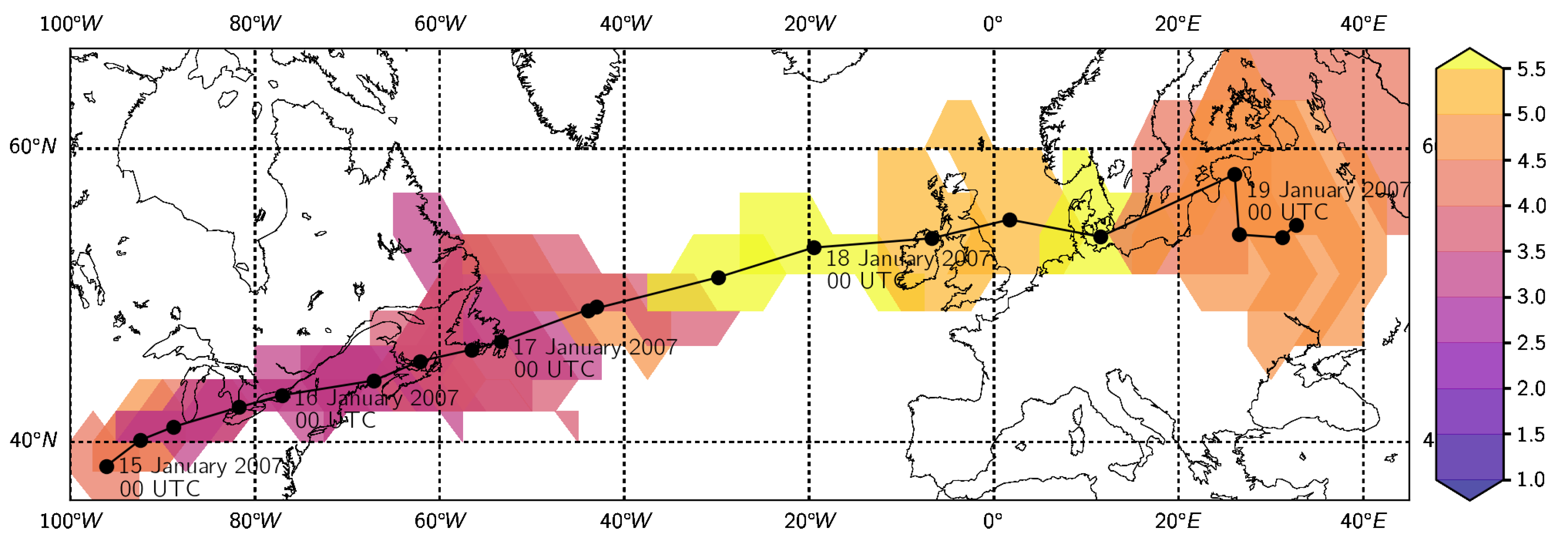
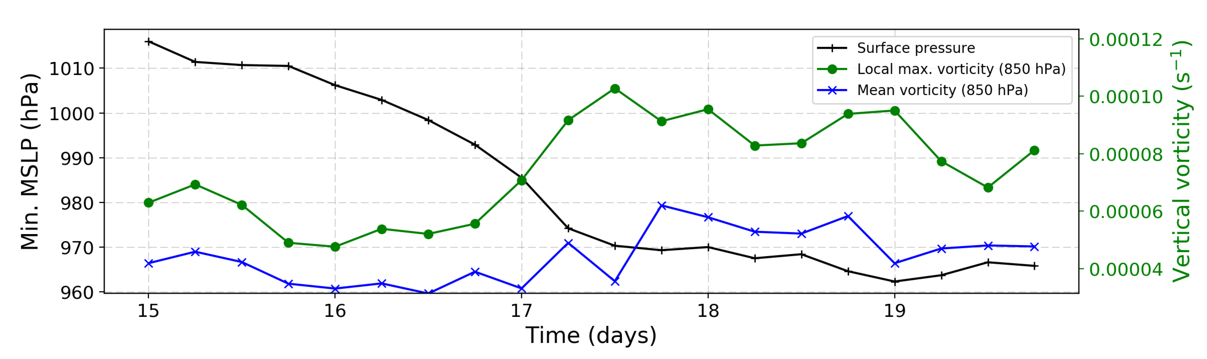
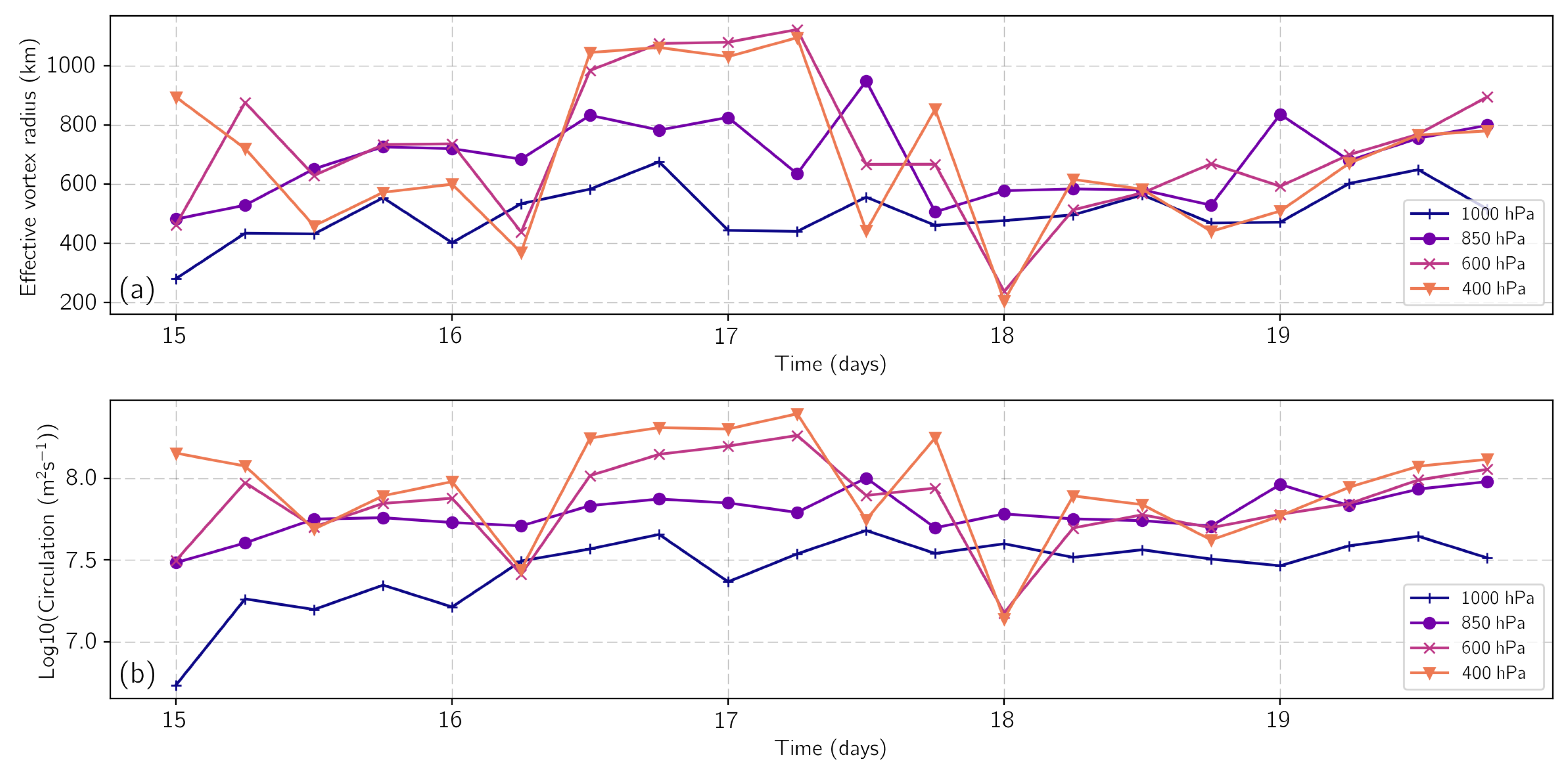
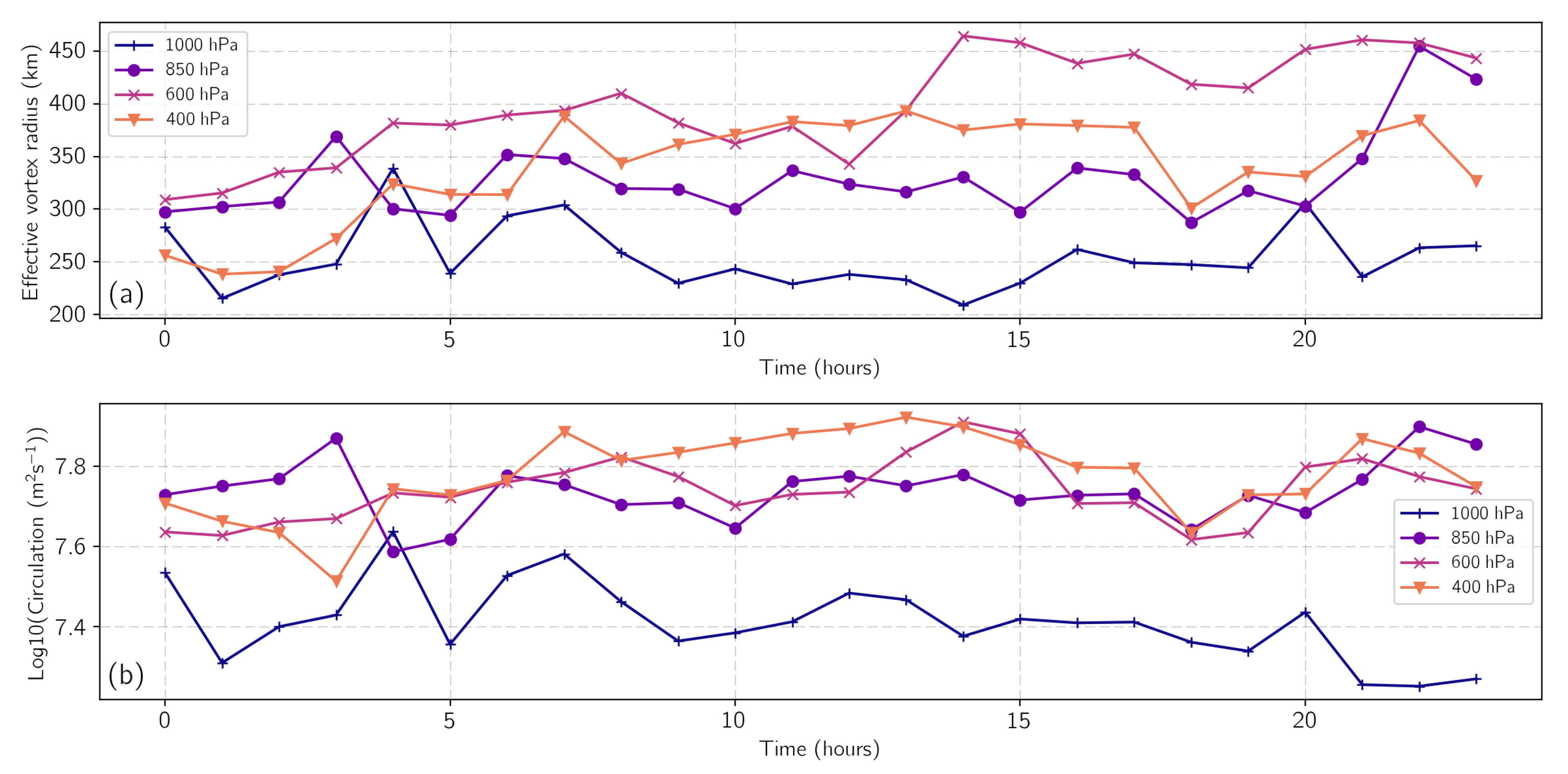
Using the -method, we can identify the vortex associated with the storm system Kyrill at different height levels of the NCEP data and track it over its lifetime. At low levels, the circulation center of Kyrill moved along a similar path as estimated for Kyrill’s core pressure in [27] (e.g., at 850 hPa, Figure 2). With respect to the vortex intensity, the mean vorticity along the path of Kyrill showed the phase of explosive cyclogenesis during 17 January 2007 (e.g., [27]), as well as the process of secondary cyclogenesis on 18 January 2007 00 UTC as described by [27] and Ludwig et al. [29] (Figure 2 and Figure 3). The high mean vorticity during Kyrill’s passage over Germany (on 18 January 2007, Figure 2) corresponded to the high winds observed at this time. The explosive cyclogenesis on 17 January 2007 was mirrored by a rapid increase in vortex radius and circulation, particularly at 400 and 600 hPa (Figure 4).
The secondary cyclogenesis was associated with a sharp minimum in both values at 400 and 600 hPa on 18 January 2007 00 UTC (Figure 4). This process was even more obvious in the vortex areas color shaded by the mean vorticity when the new vortex area was shifted to the south-east and started with less mean vorticity on 18 January 2007 00 UTC. In general, vortex size and circulation are well correlated. Moreover, after the secondary cyclogenesis on 18 January 2007, the circulations at upper pressure levels were of similar order with ms on that day with a further increase on 19 January 2007 up to about 10 ms.
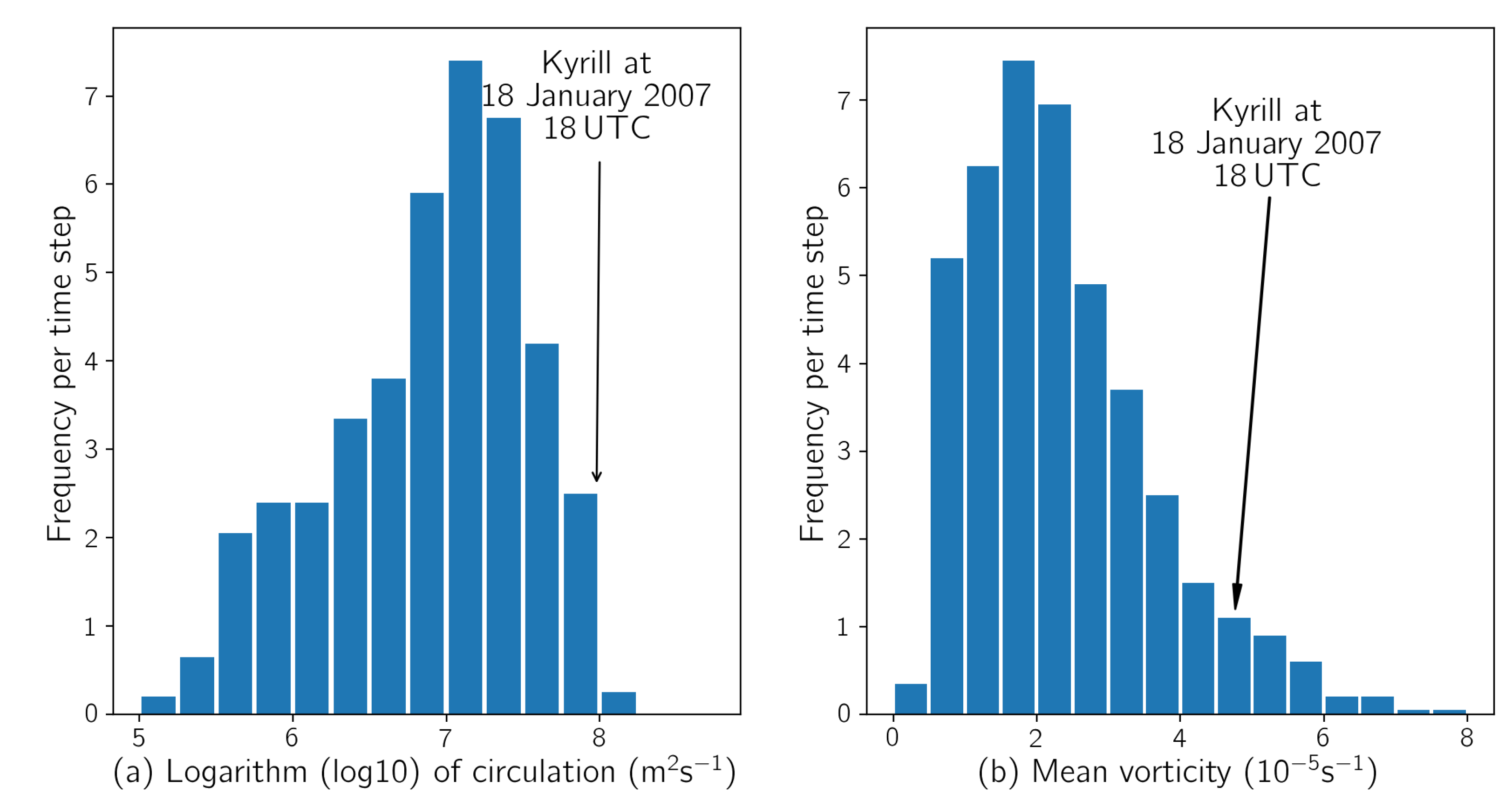
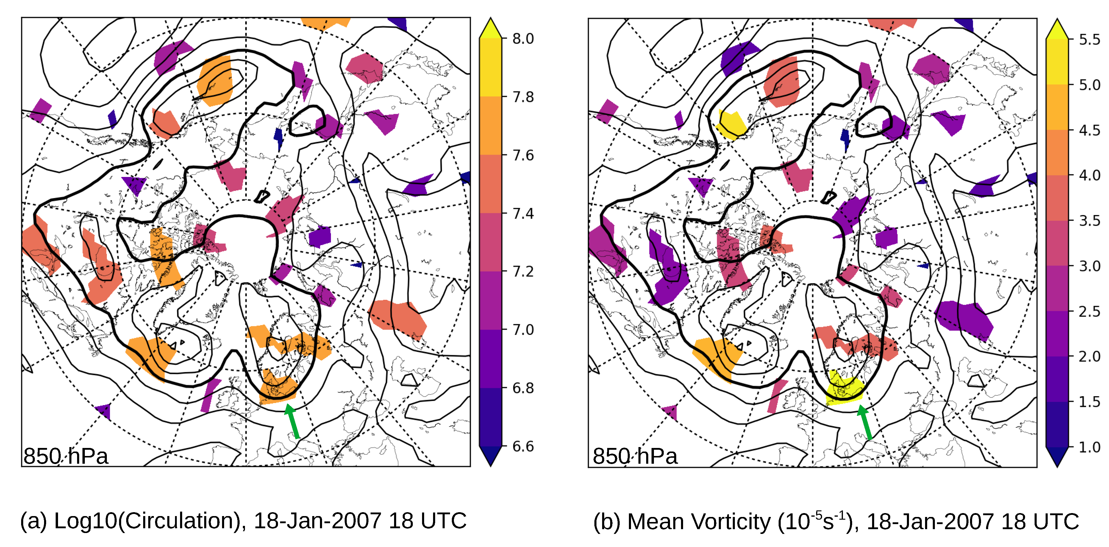
In comparison to other synoptic-scale low-pressure systems in the Northern Hemisphere during the period 15 January 00 UTC–19 January 2007 18 UTC, Kyrill was relatively strong as it moved over Germany on 18 January 2007 18 UTC. Circulation, as well as mean vorticity values of Kyrill were among the more intense systems (Figure 5). An overview of the Northern Hemisphere vortices identified with the help of the -method on 18 January 2007 at 18 UTC is given in Figure 6. In terms of circulation, Kyrill was indeed one of the stronger systems; however, there were also about 10 other systems with comparable circulation magnitudes (Figure 6a). Obviously, color shading the vortex patches fields by mean vorticity (Figure 6b) better highlighted the intensity of Kyrill at this time step. In this manner, a forecaster might take faster notice of the true intensity of a vortex that can be disguised or misled by other measures.
4.2. Kyrill in CFSR Data
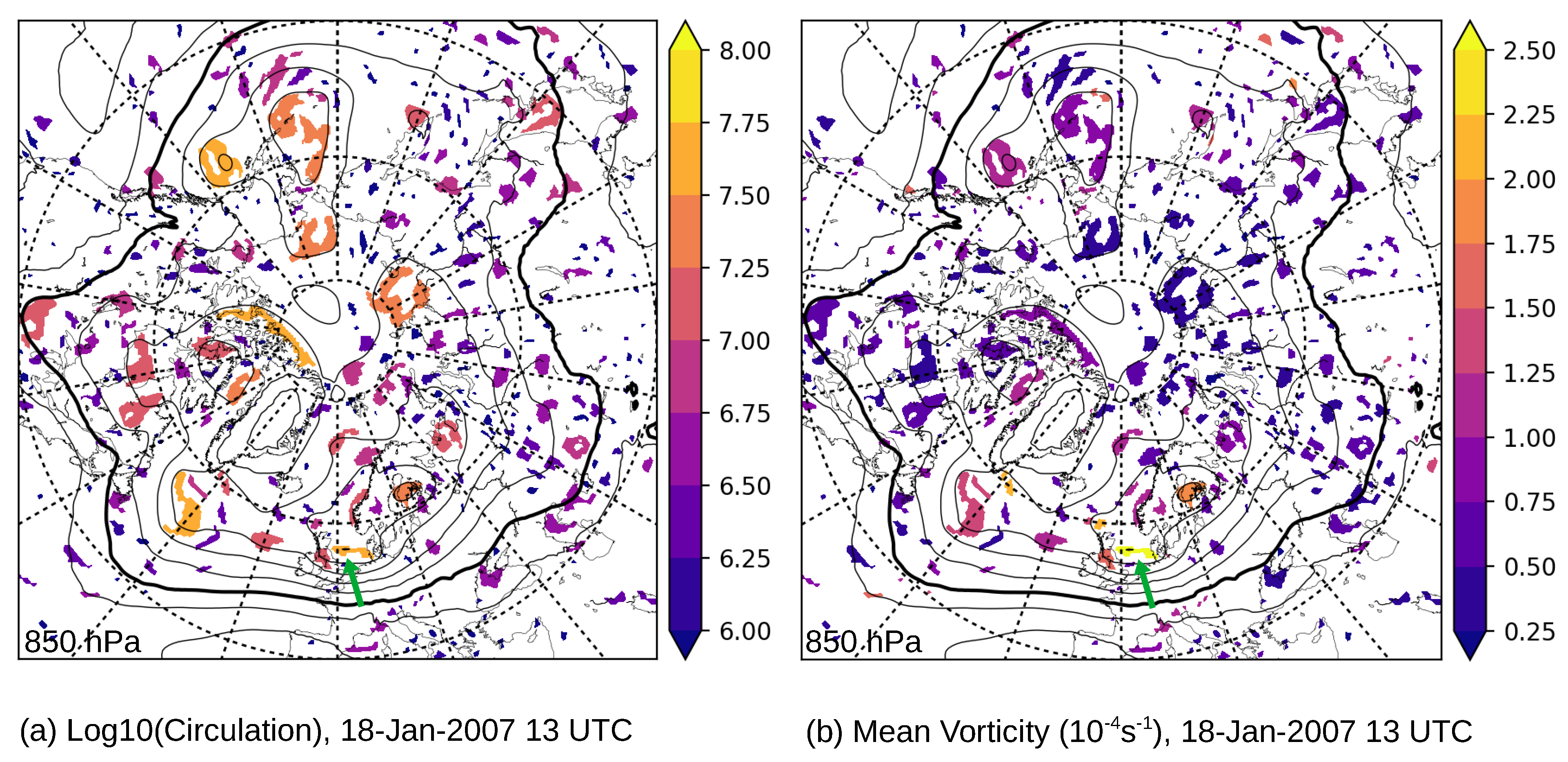
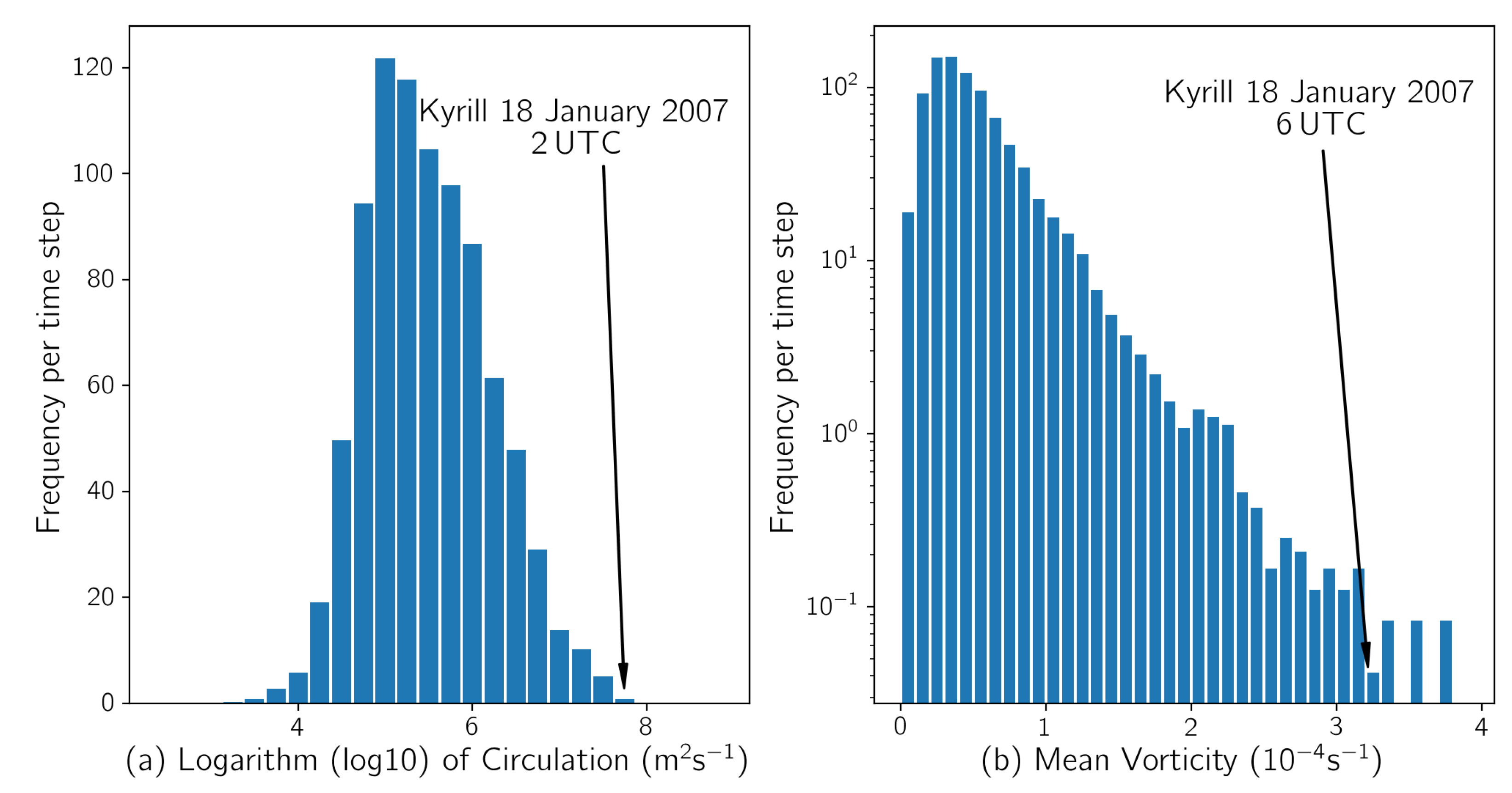
In general, the identification of vortex structures in the higher resolved CFSR data led to a larger number of vortices that had, on average, a smaller size, especially at the lower levels (Figure 7). However, the Northern Hemisphere plots for 18 January 2007 13 UTC (Figure 7) showed that Kyrill with respect to the circulation magnitude was one system among many in the hemisphere. Considering its mean vorticity, Kyrill was clearly on the intense spectrum in comparison to the other identified vortices. This was further confirmed by the frequency-intensity distributions of all Northern Hemisphere systems that occurred in the period of Kyrill’s passage over West and Central Europe that revealed a huge variety of circulation magnitudes of the identified vortices while the observed mean vorticities were in general in the sub-synoptic range with maximum values in the order of s (Figure 8).
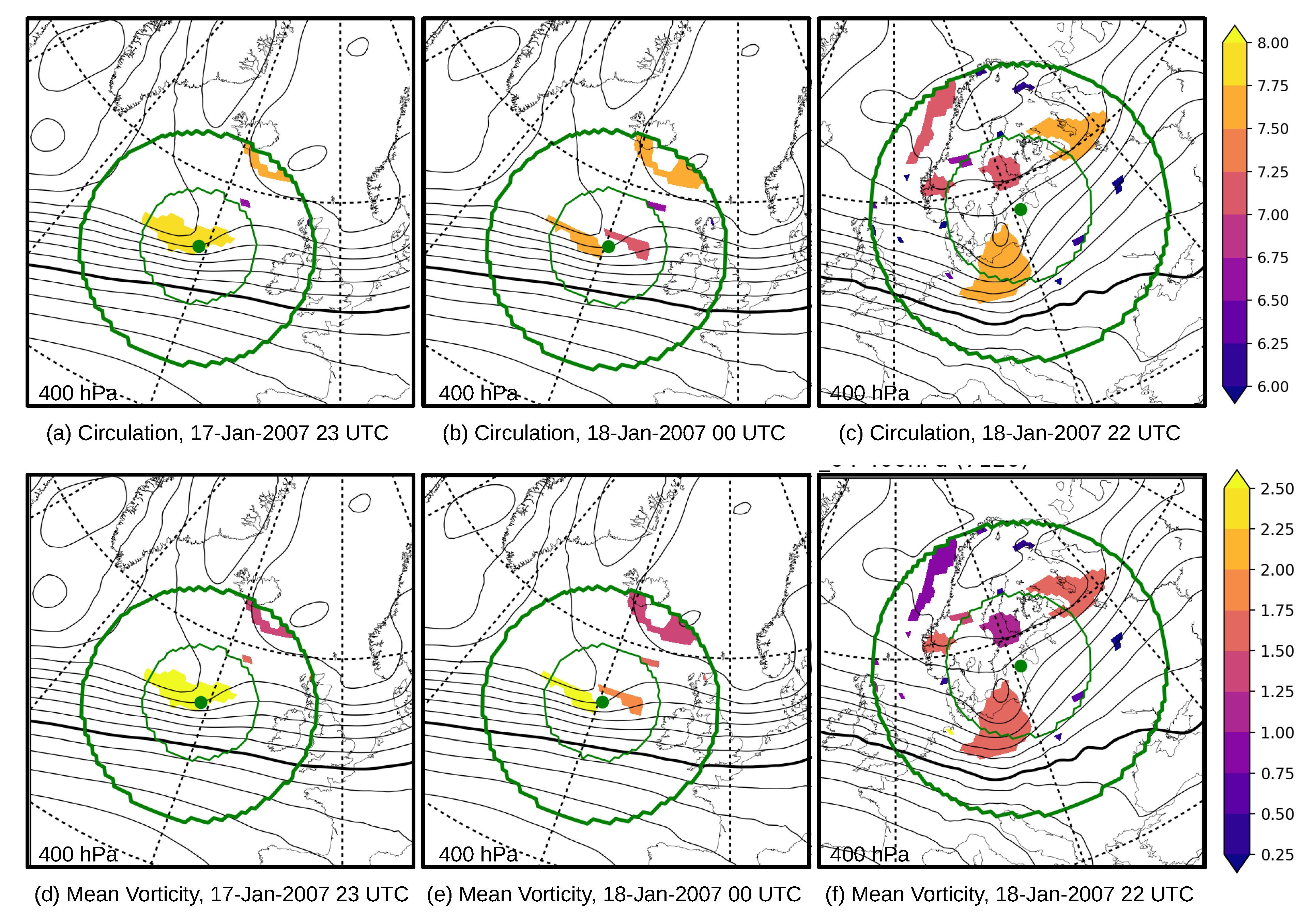
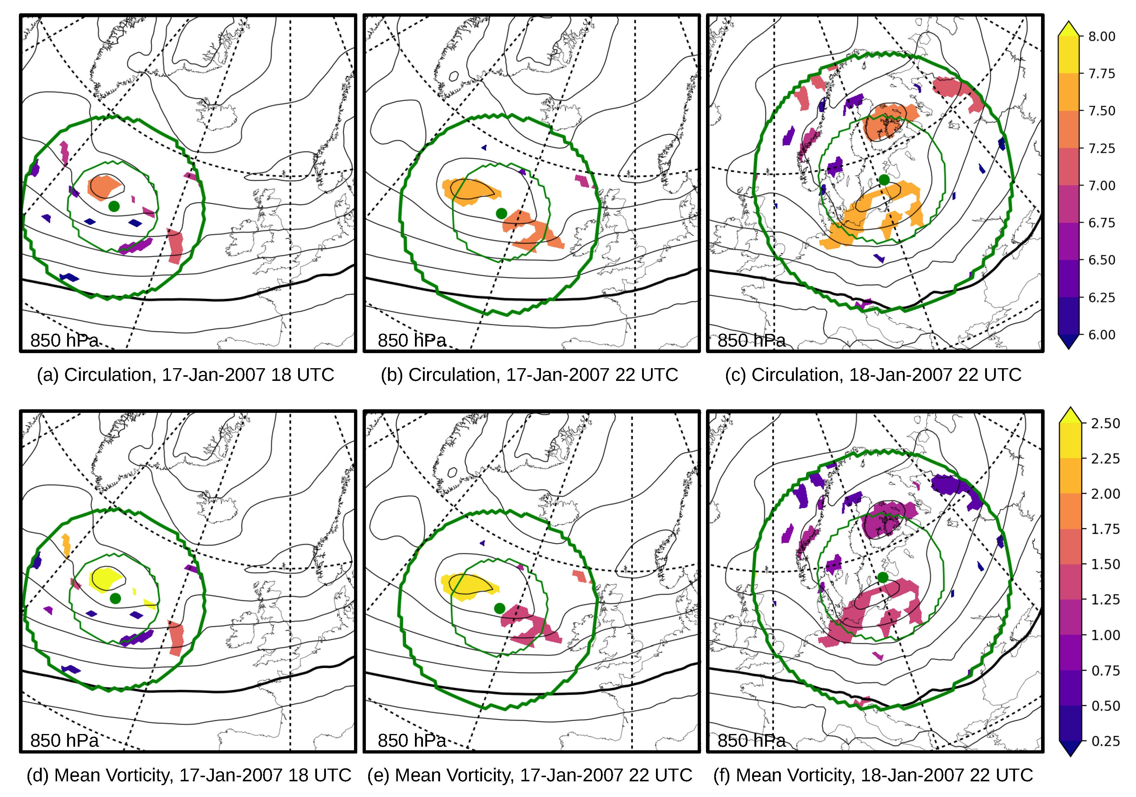
In comparison to the NCEP data, the secondary cyclogenesis of Kyrill can be observed clearly in the vortex fields derived by the CFSR data. At 400 hPa, Kyrill appeared as a large coherent system on 17 January 2007 23 UTC (Figure 9a,d). One hour later, the vortex split into two separate vortices (Figure 9b,e). These systems were weaker with respect to their circulation magnitude (Figure 9b), but of comparable magnitude regarding their mean vorticity (Figure 9e). While the western vortex moved slowly to the northeast until it dissipated on 18 January 2007 8 UTC, the eastern one moved rapidly eastwards with incipient intensification of the circulation in the morning, starting at about 5 UTC. This increase in circulation magnitude was mainly caused by a considerable increase of the vortex area. At lower pressure levels, the coherent vortex patch area observed in the upper troposphere split into several smaller-scale vortices. At 850 hPa, we observed already on 17 January 2007 18 UTC that Kyrill split into an intensive rear vortex and several vortices in the front (Figure 10a,d). The latter arranged along the fronts of Kyrill (cf., [27], their Figure 3). At this point, a tendency towards an intensification of these frontal structures was visible. At 22 UTC, the frontal vortices converged to a single system of high circulation that continued to move towards the southern North and Baltic Seas on 18 January 2007 (Figure 10b,e).
Kyrill was characterized by a rather complex occurrence of high wind speeds over Germany [27]: At first, severe (≥25 m/s) and extremely severe (>32 m/s) wind gusts occurred along a narrow elongated cold frontal rain band of Kyrill in association with a cold-season derecho along the cold front. Hereafter, a second wind event followed in the wake of the cold front, when high winds spread across northern Germany at the southern flank of the low pressure core, exhibiting a strong pressure gradient. This was also visible in Kyrill’s vortex structures that we identified with the help of the -method. Here, Germany was first affected by a vortex structure associated with the cold front of Kyrill that moved from northwest Germany to the southeast on 18 January 2007 between 15 and 19 UTC (Figure 11a–d). This rather elongated vortex had a mean vorticity of about s at 925 and 850 hPa at 14–17 UTC, indicated by the darker violet colors in Figure 11a–c, and later intensified to mean vorticities slightly higher than s. From 18 UTC onward, a consecutive vortex (Figure 11, yellow-orange vortex structure in the three lowest levels) followed from the North Sea that merged with the northern vortex of Kyrill until 19 January 2007 00 UTC, corresponding to the time period when the second wind maximum was displayed in [27]. Finally, the vortex area extended far into southern Germany (Figure 9c,f) and continued to grow on 19 January 2007. At this point, the mean vorticity was decreased (Figure 9f) in comparison to the previous hours, while the circulation (Figure 9c) still remained in the same order of magnitude. This difference in the intensity measures can be explained by the fact that the size of Kyrill grew over time, and since the circulation magnitude depended directly on the area, Kyrill’s circulation remained similar. The mean vorticity on the other hand mirrored rather the (local) impact related intensity that had already a weakening tendency at the 850 hPa level.
In summary, the vortex structures associated with Kyrill crossed large portions of Germany and thus reflected the high impact of Kyrill, in agreement with [27]. The cold front appeared as a separate vortex in the lower levels and merged at upper levels with the main vortex representing Kyrill’s center (Figure 11). The other way around, the upper-tropospheric larger-scale vortex area split to several smaller-scale vortex structures in the lower troposphere. However, the total positive circulation of Kyrill’s vortex structures had a similar magnitude of ms to the NCEP vortex (Figure 12) while the effective radius derived by adding up the areas of the associated vortex structures and applying Equation (10) was reduced to 300–400 km compared to about 500–600 km for the NCEP vortex. This reduction in vortex size while the circulation remained approximately equal also explains the higher values of the vortex mean vorticities in comparison to the NCEP data.
4.3. Kyrill in COSMO Data
The COSMO simulation covered the passage of Kyrill over Germany during the period from 18 January 2007 14 UTC–19 January 2007 00 UTC. In the highly-resolved COSMO data (horizontal grid spacing of about 2.8 km), the -method detected a huge number of vortices with a broad spectrum of circulations and mean vorticities (Figure 13). The larger-scale vortices that we identified in the coarser NCEP and CFSR datasets fragmented into numerous smaller-scale vortices. Nonetheless, the sum of the total positive circulation of all vortices identified in the COSMO data within a certain radius around Kyrill’s NCEP location remained of the same magnitude compared to the total circulation of Kyrill in the NCEP and CFSR data at the upper levels (Figure 14b). As in the other datasets, the area covered by vortices associated with Kyrill increased with height (Figure 14a).
The development of the vortex intensity differed by comparing COSMO and CSFR data. At 850 hPa, the vortex based on COSMO data started to weaken shortly after 18 January 2007 18 UTC, whereas there was an increase of its circulation based on NCEP and CSFR data. The weakening in COSMO data, also indicated at 600 hPa, was related to the movement of Kyrill across the analysis domain: this caused an increase of the sum of the circulation until the vortex started to leave the domain, and the sum of circulations decreased again (Figure 14b).
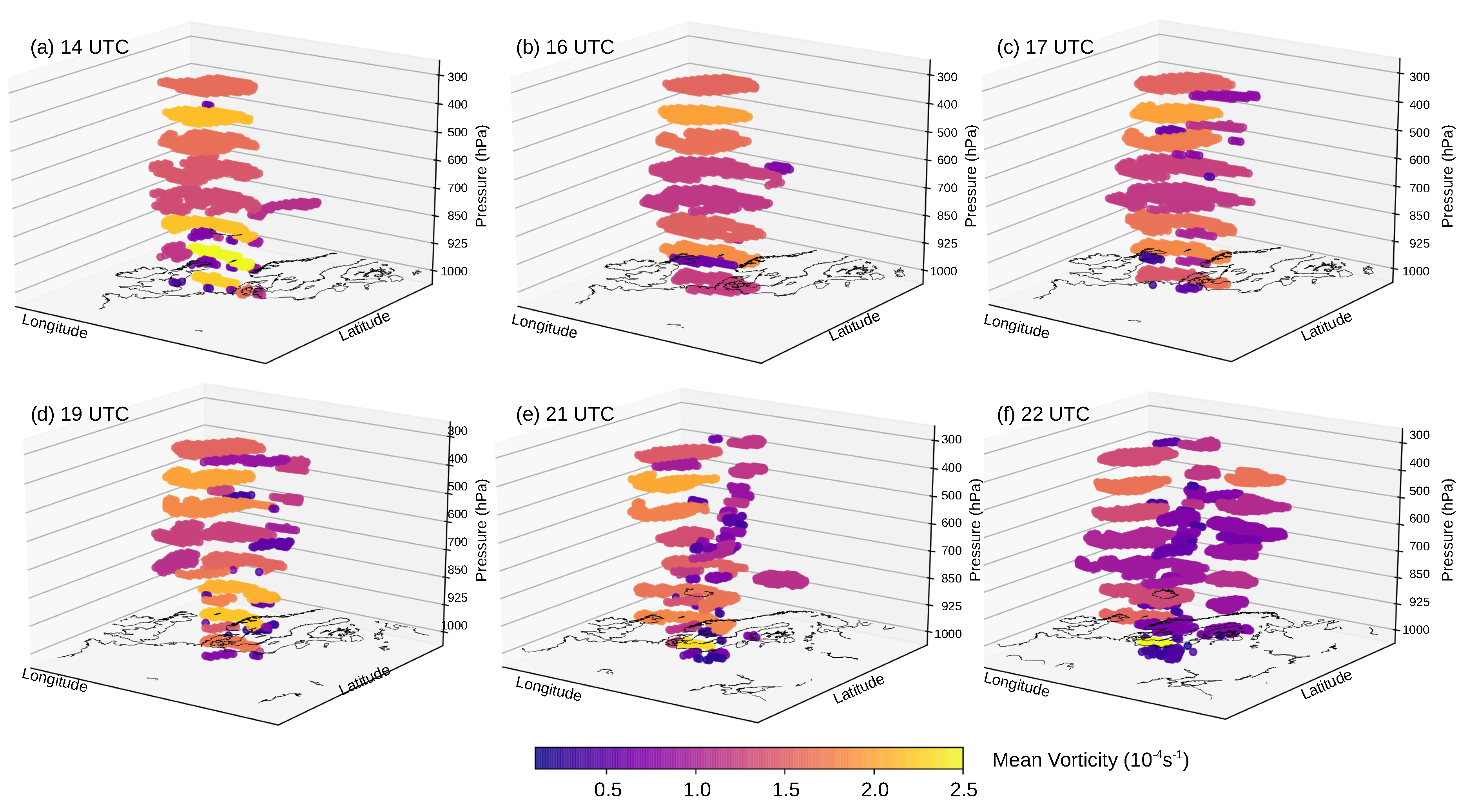
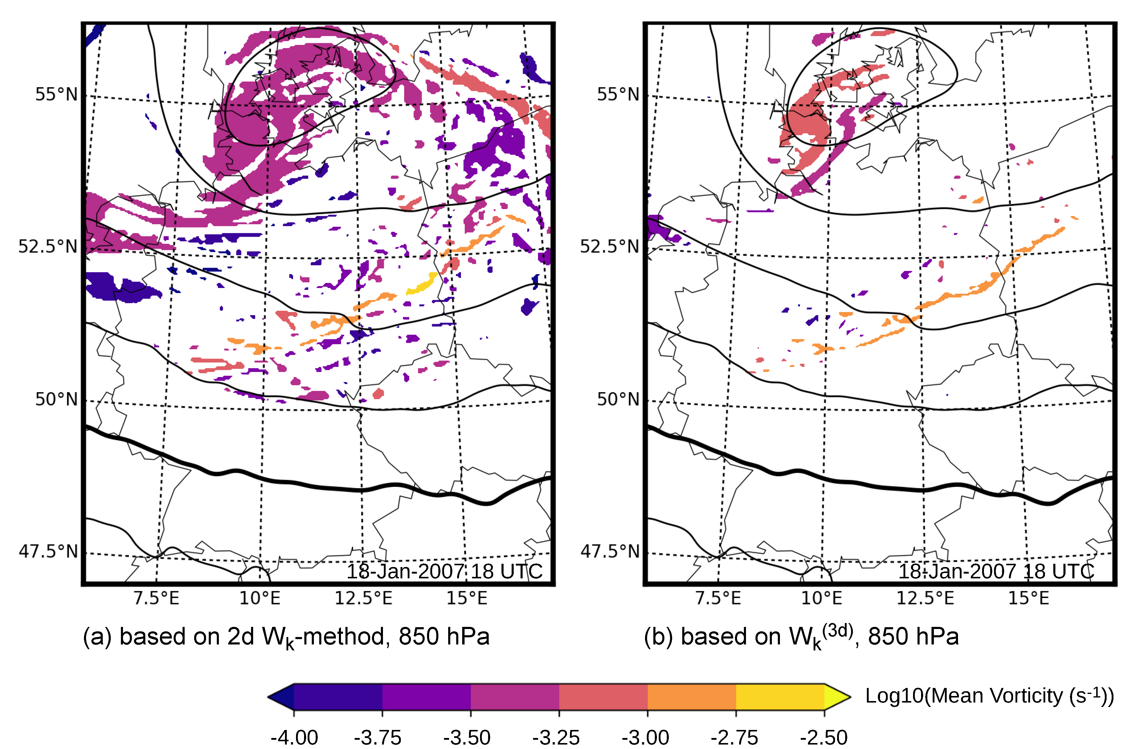
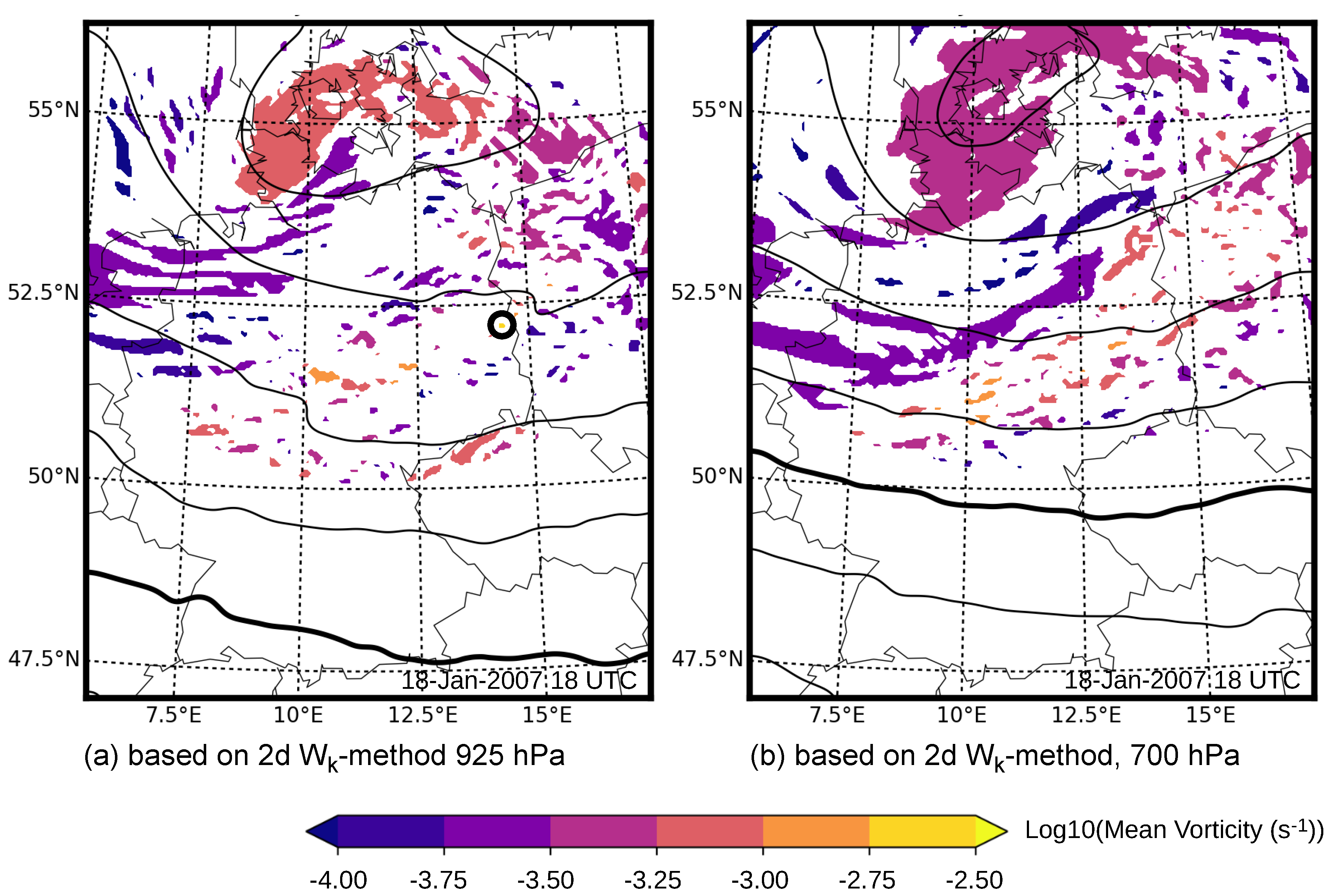
A closer look at the vortex structures in the COSMO field indicated separate areas of different vortices across Germany. There was an area of small-scale bands of vortices close to the cold front of Kyrill (e.g., at 18 UTC, 850 hPa, Figure 15a). Here, cold-frontal convection was detected that was also obvious in radar imagery [27,28]. The cold frontal convection formed several bowing segments that were also visible in the vortex fields. The most prominent bowing segments were detected as separate vortices using the -method. These bowing segments were the most intense vortices at that time as indicated by their high mean vorticity (Figure 15a). Swaths of high maximum wind gusts derived from the model ([29], their Figure 8) were located in the path of the detected bowing segments. At 925 hPa, i.e., less than 500 m above the ground, the structure of the cold front convection almost disappeared. Bowing segments could not be seen at this level (Figure 16a). However, there were a few, small-scale vortices with a diameter of about 10 km that could be related to bookend vortices [40] at the ends of bowing segments (highlighted by the black circle in Figure 16a). Although these vortices were almost too small to be resolved at the given model resolution of 2.8 km, they were detected over a time period of about one hour, during which they moved together with the bowing segment detected at higher levels. Above 850 hPa, we also observed less pronounced vortices along the cold front convection. This indicates that these vortices were rather shallow. Additionally, the detected vortices at 700 hPa were located east of the vortices detected at 850 hPa (Figure 16b). Therefore, the cold-frontal convection was strongly tilted due to the strong westerly shear [28].
In summary, the -method detected vortices related to the cold-frontal convection at different scales. Likewise, it indicated that the convection was rather shallow and strongly tilted. In the wake of the cold-frontal convection, only very few vortices were detected. This area of almost no vortices corresponded to the region of the convective cold pool [28]. Finally, there were larger scale vortices close to the center of Kyrill. We concluded that the -method was able to identify vortices of different scales in the same model field. While most of the detected vortices fragmented near the ground, some large vortices detected at high levels also appeared as large vortices near the ground.
Given the small scale of the detected vortices in the COSMO data and the related importance of the vertical coordinate, the two-dimensional -method that only accounted for horizontal vortices can give an incomplete view of the vortex structures. Hence, we additionally compared the vortex images of the two-dimensional -method with the ones based on the complete structures that were identified with the help of the three-dimensional -method and a higher threshold of 1.1. The main difference was that many, mostly weak vortices disappeared in the images of the -method, in particular in the lower troposphere (e.g., at 850 hPa, Figure 15b). However, at the same time, the cold-frontal convective structure such as bowing segments was more pronounced compared to the two-dimensional -method, and the bookend vortices close to the ground were still detected.
5. Discussion and Conclusions
In this work, we analyzed a high-impact extratropical cyclone with respect to its vortex properties in datasets of different horizontal grid spacing, covering the synoptic to the convective scales. The vortex properties were computed with the help of a single kinematic vortex identification method (-method). This method was based on the dimensionless kinematic vorticity number that differentiates between rotation-prevailing, i.e., vortices, vs. deformation-prevailing regions of the flow field. The main outcomes of this study were:
- The -method was able to identify vortices throughout differently-resolved datasets in a reasonable manner, even at the convective scale.
- The identified vortices were in general larger in the upper troposphere and fragmented into smaller-scales in the lower troposphere.
- The synoptic-scale storm system was composed of a large spectrum of vortex structures with varying horizontal scales and intensities.
- However, the total circulation of the system remained approximately constant across the scales, while the magnitude of the rather impact-related mean vorticity of the single vortices could increase considerably with increasing resolution.
The most surprising and, for us, impressive result was the almost complete conservation of the circulation throughout the different datasets. This has some implications with respect to the interpretation of vortex intensities in climate change studies: if an increase in the synoptic-scale circulations were observed in future scenarios, the intensity of smaller-scale embedded vortices could increase, as well. Though it was not clear which intensity measure was the best and this problem possibly depends significantly on the research question, we were positively surprised by the performance of circulation and mean vorticity. Color shading the vortices by their mean vorticity on the other hand seemed to highlight the intense, impact-related vortices such as the ones that occurred along Kyrill’s cold front. Though the plots needed scale-dependent adjustments considering the vorticity range, they could still be a useful tool, especially with respect to the forecast of high-impact weather. However, besides single case studies, a detailed climatological analysis should be done in future work to further explore the benefits of the -method.
We already knew that the vorticity was a scale-dependent variable, e.g., [12], and that vorticity-related measures such as the potential vorticity were scale-dependent, as in [41], who studied the sensitivity of resolution on a tropical cyclone with horizontal grid spacings between 1 and 8 km. With our study, we can confirm that the vorticity magnitudes indeed increased with increasing resolutions. Additionally, we can explicitly calculate the distribution of mean vorticity and circulation magnitudes. The sizes of the resolved vortices showed a large spectrum of effective radii, in particular in the higher-resolved datasets. Even in the high-resolution COSMO data, we still observed a (sub-)synoptic-scale vortex that represented the central core of Kyrill and a multitude of vortices with different scales that were associated with fronts and convective cells. We summarize these important results in Table 1.
Our observation that the size of extratropical cyclones in general increased with height was also found in Lim and Simmonds [42], who based their vortex identification on the Laplacian of the pressure (the Laplacian of pressure is proportional to the geostrophic vorticity). We can now further confirm that this general increase also occurred in data with higher resolution. However, Lim and Simmonds [42] did not describe a possible fragmentation of an upper-level vortex into smaller-scale vortices in the lower troposphere. Those structures were perhaps missing due to the removal of less intense systems in advance. The fragmentation was also documented in some example cases given in [43], who used a 4D tracking algorithm to study the four-dimensional structure of Southern Hemisphere low-pressure systems based on the anomaly fields of the vertical vorticity. Understanding the reasons for this fragmentation and its connection to viscous processes could be an interesting topic for future studies, especially since the contraction of the vortex area led to an intensification due to the (quasi-)conservation of the circulation.
Finally, we were able to display some characteristics of the high-impact event addressed in the literature. The -method can identify the processes of explosive intensification of Kyrill and secondary cyclogenesis in accordance with the publications of [27,29]. With the additional knowledge of the vortex size and the use of different intensity measures, the visualization of these processes was quite clear, especially the secondary cyclogenesis and even in the coarsely-resolved NCEP data.
At high resolution, our method highlighted deep moist convection, including information on the convective storm mode such as bowing segments and bookend vortices and regions of high winds. A surprising result was the different identification of vortex structures for the two-dimensional and the three-dimension -method. Although the -method identified the stronger vortices with higher mean vorticities in the lower levels similar to the 2D -method, it is important to understand what the unidentified vortices were. These were likely related to convective cells or waves with upward and downward motions that appeared as a vortex in the 2D fields. The two-dimensional kinematic vorticity number assumed that the vortex rotated around an approximately vertical axis and only compared the vertical vorticity with the deformational flow components at the horizontal level. Kyrill was a storm system that interacted with the upper-level jet stream [29]. Hence, the environment of the convection was characterized by strong vertical wind shear. This also implied large horizontal vorticity components. Due to up- and down-drafts, these vorticity lines were tilted up- or downwards, generating vertical vorticity. The magnitude of the vertical vorticity was in large parts of the field higher than the strain-rate, and hence, a vortex was identified. A change to the three-dimensional -method revealed that the associated three-dimensional strain-rates were higher or at least of comparable order to the vorticity vector components.
In summary, the -method performed well in the data of different resolutions and at different height levels. The proposed color shading by intensity measures seemed to highlight potentially high-impact vortices. The method might be of interest to a variety of topics, including teaching, mesoscale meteorology, storm dynamics, climate research, and storm risk estimation. Therefore, the -method is a promising tool for various future applications.
Author Contributions
Conceptualization, L.S. and C.P.G.; methodology, L.S.; software, L.S.; data curation, P.L.; formal analysis, C.P.G. and L.S.; writing, original draft preparation, L.S., C.P.G., and P.L; writing, review and editing, L.S., C.P.G., and P.L.; visualization, L.S.
Funding
We acknowledge the support of the German Research Foundation and the Open Access Publication Fund of the Freie Universität Berlin. P.L. thanks the Helmholtz initiative REKLIM for funding.
Acknowledgments
We thank the two anonymous reviewers for their valuable comments that improved the manuscript. Many thanks also to the Academic Editors of the journal for the support. The publication of this article was funded by Freie Universität Berlin.
Conflicts of Interest
The authors declare no conflict of interest.
References
- Jeong, J.; Hussain, F. On the identification of a vortex. J. Fluid Mech. 1995, 285, 69–94. [Google Scholar] [CrossRef]
- Neu, U.; Akperov, M.G.; Bellenbaum, N.; Benestad, R.; Blender, R.; Caballero, R.; Cocozza, A.; Dacre, H.F.; Feng, Y.; Fraedrich, K.; et al. IMILAST: A community effort to intercompare extratropical cyclone detection and tracking algorithms. Bull. Am. Meteorol. Soc. 2013, 94, 529–547. [Google Scholar] [CrossRef]
- Wernli, H.; Schwierz, C. Surface Cyclones in the ERA-40 Dataset (1958–2001). Part I: Novel Identification Method and Global Climatology. J. Atmos. Sci. 2006, 63, 2486–2507. [Google Scholar] [CrossRef]
- Schneidereit, A.; Blender, R.; Fraedrich, K. A radius-depth model for midlatitude cyclones in reanalysis data and simulations. Q. J. R. Meteorol. Soc. 2010, 136, 50–60. [Google Scholar] [CrossRef]
- Murray, R.J.; Simmonds, I. A numerical scheme for tracking cyclone centres from digital data. Aust. Meteorol. Mag. 1991, 39, 167–180. [Google Scholar]
- Sinclair, M.R. An objective cyclone climatology for the Southern Hemisphere. Mon. Weather. Rev. 1994, 122, 2239–2256. [Google Scholar] [CrossRef]
- Flaounas, E.; Kotroni, V.; Lagouvardos, K.; Flaounas, I. CycloTRACK (v1.0)—Tracking winter extratropical cyclones based on relative vorticity: sensitivity to data filtering and other relevant parameters. Geosci. Model Dev. 2014, 7, 1841–1853. [Google Scholar] [CrossRef]
- Leckebusch, G.C.; Renggli, D.; Ulbrich, U. Development and application of an objective storm severity measure for the Northeast Atlantic region. Meteorol. Z. 2008, 17, 575–587. [Google Scholar] [CrossRef]
- Sinclair, M.R. Objective identification of cyclones and their circulation intensity, and climatology. Weather. Forecast. 1997, 12, 595–612. [Google Scholar] [CrossRef]
- Schielicke, L.; Névir, P.; Ulbrich, U. Kinematic vorticity number—A tool for estimating vortex sizes and circulations. Tellus A 2016, 68, 29464. [Google Scholar] [CrossRef]
- Ulbrich, U.; Leckebusch, G.; Pinto, J. Extra-tropical cyclones in the present and future climate: A review. Theor. Appl. Climatol. 2009, 96, 117–131. [Google Scholar] [CrossRef]
- Hodges, K.I.; Hoskins, B.J.; Boyle, J.; Thorncroft, C. A comparison of recent reanalysis datasets using objective feature tracking: Storm tracks and tropical easterly waves. Mon. Weather. Rev. 2003, 131, 2012–2037. [Google Scholar] [CrossRef]
- Müller, A.; Névir, P.; Schielicke, L.; Hirt, M.; Pueltz, J.; Sonntag, I. Applications of point vortex equilibria: Blocking events and the stability of the polar vortex. Tellus A 2015, 67, 29184. [Google Scholar] [CrossRef]
- Hirt, M.; Schielicke, L.; Müller, A.; Névir, P. Statistics and dynamics of blockings with a point vortex model. Tellus Dyn. Meteorol. Oceanogr. 2018, 70, 1–20. [Google Scholar] [CrossRef] [Green Version]
- Hunt, J.C.; Wray, A.; Moin, P. Eddies, streams, and convergence zones in turbulent flows. In Studying Turbulence Using Numerical Simulation Databases–II, Proceedings of the Summer Program 1988, Report CTR-S88; Center of Turbulence Research, Stanford University: Stanford, CA, USA, 1988; pp. 193–208. [Google Scholar]
- Chong, M.; Perry, A.E.; Cantwell, B. A general classification of three-dimensional flow fields. Phys. Fluids Fluid Dyn. 1990, 2, 765–777. [Google Scholar] [CrossRef]
- Okubo, A. Horizontal dispersion of floatable particles in the vicinity of velocity singularities such as convergences. In Deep Sea Research and Oceanographic Abstracts; Elsevier: Amsterdam, The Netherlands, 1970; Volume 17, pp. 445–454. [Google Scholar]
- Weiss, J. The dynamics of enstrophy transfer in two-dimensional hydrodynamics. Phys. Nonlinear Phenom. 1991, 48, 273–294. [Google Scholar] [CrossRef]
- Truesdell, C. Two measures of vorticity. J. Ration. Mech. Anal. 1953, 2, 173–217. [Google Scholar] [CrossRef]
- Truesdell, C. The Kinematics of Vorticity; Indiana University Press: Bloomington, Indiana, 1954; p. 232. [Google Scholar]
- Thompson, R.L.; Bacchi, R.D.A.; Machado, F.J. What is a vortex? In Proceedings of the 20th International Congress of Mechanical Engineering, Gramado, Brazil, 15–20 November 2009.
- Dunkerton, T.; Montgomery, M.; Wang, Z. Tropical cyclogenesis in a tropical wave critical layer: Easterly waves. Atmos. Chem. Phys. 2009, 9, 5587–5646. [Google Scholar] [CrossRef]
- Tory, K.J.; Dare, R.; Davidson, N.; McBride, J.; Chand, S. The importance of low-deformation vorticity in tropical cyclone formation. Atmos. Chem. Phys. 2013, 13, 2115–2132. [Google Scholar] [CrossRef] [Green Version]
- Markowski, P.M.; Richardson, Y.; Majcen, M.; Marquis, J.; Wurman, J. Characteristics of the wind field in three nontornadic low-level mesocyclones observed by the Doppler on Wheels radars. E J. Sev. Storms Meteorol. 2011, 6, 410. [Google Scholar]
- Schielicke, L. Scale-Dependent Identification and Statistical Analysis of Atmospheric Vortex Structures in Theory, Model and Observation. Ph.D. Thesis, Freie Universität Berlin, Berlin, Germany, 2017. [Google Scholar]
- Munich Re, Geo Risks Research, NatCatSERVICE . Loss Events in Europe 1980–2014: 10 Costliest Winter Storms Ordered by Insured Losses. 2015. Available online: https://www.munichre.com/site/wrap/get/documents_E2089112740/mr/assetpool.shared/Documents/5_Touch/_NatCatService/Significant-Natural-Catastrophes/2014/10-costliest-winter-storms-ordered-by-insured-losses.pdf (accessed on 1 August 2007).
- Fink, A.H.; Brücher, T.; Ermert, V.; Krüger, A.; Pinto, J.G. The European storm Kyrill in January 2007: Synoptic evolution, meteorological impacts and some considerations with respect to climate change. Nat. Hazards Earth Syst. Sci. 2009, 9, 405–423. [Google Scholar] [CrossRef]
- Gatzen, C.; Púčik, T.; Ryva, D. Two cold-season derechoes in Europe. Atmos. Res. 2011, 100, 740–748. [Google Scholar] [CrossRef]
- Ludwig, P.; Pinto, J.G.; Hoepp, S.A.; Fink, A.H.; Gray, S.L. Secondary cyclogenesis along an occluded front leading to damaging wind gusts: Windstorm Kyrill, January 2007. Mon. Weather. Rev. 2015, 143, 1417–1437. [Google Scholar] [CrossRef]
- National Centers for Environmental Prediction/National Weather Service/NOAA/U.S. Department of Commerce. NCEP/DOE Reanalysis 2 (R2). 2000. Available online: http://rda.ucar.edu/datasets/ds091.0/ (accessed on 24 June 2019).
- Kanamitsu, M.; Ebisuzaki, W.; Woollen, J.; Yang, S.K.; Hnilo, J.; Fiorino, M.; Potter, G. NCEP–DOE AMIP-II Reanalysis (R-2). Bull. Am. Meteorol. Soc. 2002, 83, 1631–1644. [Google Scholar] [CrossRef]
- Saha, S.; Moorthi, S.; Pan, H.L.; Wu, X.; Wang, J.; Nadiga, S.; Tripp, P.; Kistler, R.; Woollen, J.; Behringer, D.; et al. NCEP Climate Forecast System Reanalysis (CFSR) 6-hourly Products, January 1979 to December 2010. Available online: https://doi.org/10.5065/D6513W89 (accessed on 11 August 2017).
- Saha, S.; Moorthi, S.; Pan, H.L.; Wu, X.; Wang, J.; Nadiga, S.; Tripp, P.; Kistler, R.; Woollen, J.; Behringer, D.; et al. The NCEP Climate Forecast System Reanalysis. Bull. Am. Meteorol. Soc. 2010, 91, 1015–1058. [Google Scholar] [CrossRef]
- Rockel, B.; Will, A.; Hense, A. The regional climate model COSMO-CLM (CCLM). Meteorol. Z. 2008, 17, 347–348. [Google Scholar] [CrossRef]
- Hunter, J.D. Matplotlib: A 2D graphics environment. Comput. Sci. Eng. 2007, 9, 90–95. [Google Scholar] [CrossRef]
- Whitaker, J. Basemap Matplotlib Toolkit. 2011. Available online: http://matplotlib.github.com/basemap/ (accessed on 2 September 2019).
- Wessel, P. and Smith, W.H.F. A global, self-consistent, hierarchical, high-resolution shoreline database. J. Geophys. Res. Solid Earth 1996, 101, 8741–8743. [Google Scholar] [CrossRef]
- Fortak, H. Vorlesungen über Theoretische Meteorologie—Kinematik der Atmosphäre; Institut für Theoretische Meteorologie der Freien Universität Berlin: Berlin, Germany, 1967; p. 128. [Google Scholar]
- Batchelor, C.K.; Batchelor, G. An Introduction to Fluid Dynamics, 14th ed.; Cambridge Mathematical Library; Cambridge University Press: Cambridge, UK, 2000; p. 658. [Google Scholar]
- Markowski, P.; Richardson, Y. Mesoscale Meteorology in Midlatitudes; John Wiley & Sons: Hoboken, NJ, USA, 2011; Volume 2. [Google Scholar]
- Gentry, M.S.; Lackmann, G.M. Sensitivity of simulated tropical cyclone structure and intensity to horizontal resolution. Mon. Weather. Rev. 2010, 138, 688–704. [Google Scholar] [CrossRef]
- Lim, E.P.; Simmonds, I. Southern Hemisphere winter extratropical cyclone characteristics and vertical organization observed with the ERA-40 data in 1979–2001. J. Clim. 2007, 20, 2675–2690. [Google Scholar] [CrossRef]
- Lakkis, S.G.; Canziani, P.; Yuchechen, A.; Rocamora, L.; Caferri, A.; Hodges, K.; O’Neill, A. A 4D feature-tracking algorithm: A multidimensional view of cyclone systems. Q. J. R. Meteorol. Soc. 2019, 145, 395–417. [Google Scholar] [CrossRef]
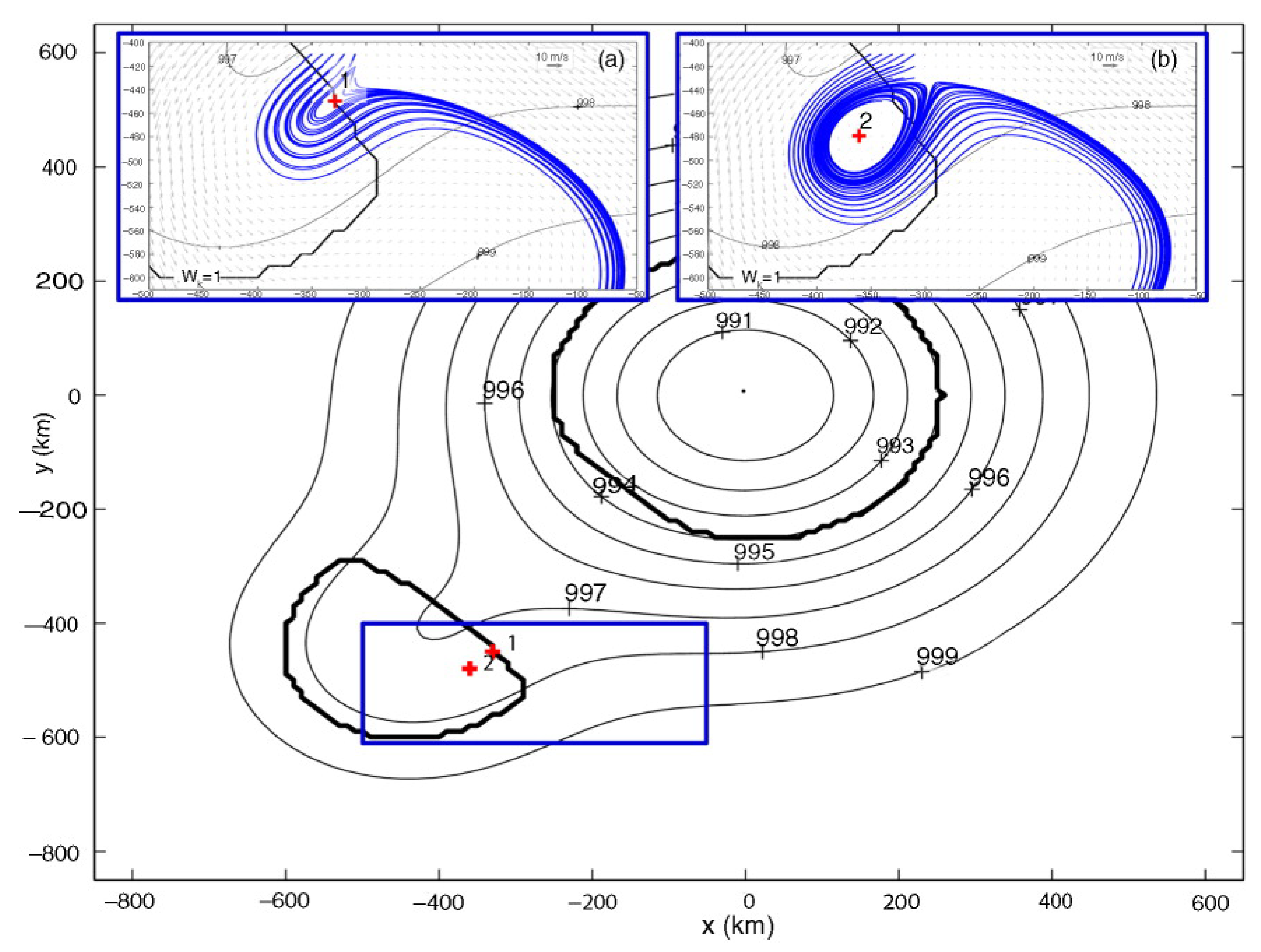
Figure 1.
Horizontal streamline patterns around two points labeled 1 and 2 with different values in a field of two superpositioned low pressure systems. Thin black contours are isobars, and thick black contours are equal to . The blue box indicates the region plotted in the insets. (a) Streamlines (blue) around Point 1 with at the vortex core boundary, and (b) streamlines (blue) around Point 2 with inside the vortex core. Gray arrows are the horizontal wind vectors around 1 and 2, respectively. Figure was originally published in Schielicke et al (2016, their Figure 8) [10] under the Creative Commons Attribution 4.0 International License (http://creativecommons.org/licenses/by/4.0/).

Figure 2.
Area of Kyrill derived from NCEP data color shaded by its mean vorticity (in 10s) at 850 hPa followed over its lifetime. Black dots indicate the circulation center of Kyrill at six-hourly time steps.
Figure 2.
Area of Kyrill derived from NCEP data color shaded by its mean vorticity (in 10s) at 850 hPa followed over its lifetime. Black dots indicate the circulation center of Kyrill at six-hourly time steps.

Figure 3.
Minimum of mean sea level pressure (MSLP) observed inside Kyrill’s area (black line) and mean vorticity averaged over Kyrill’s area (blue line), as well as local maximum vorticity observed inside the area. Properties derived from NCEP data.
Figure 3.
Minimum of mean sea level pressure (MSLP) observed inside Kyrill’s area (black line) and mean vorticity averaged over Kyrill’s area (blue line), as well as local maximum vorticity observed inside the area. Properties derived from NCEP data.

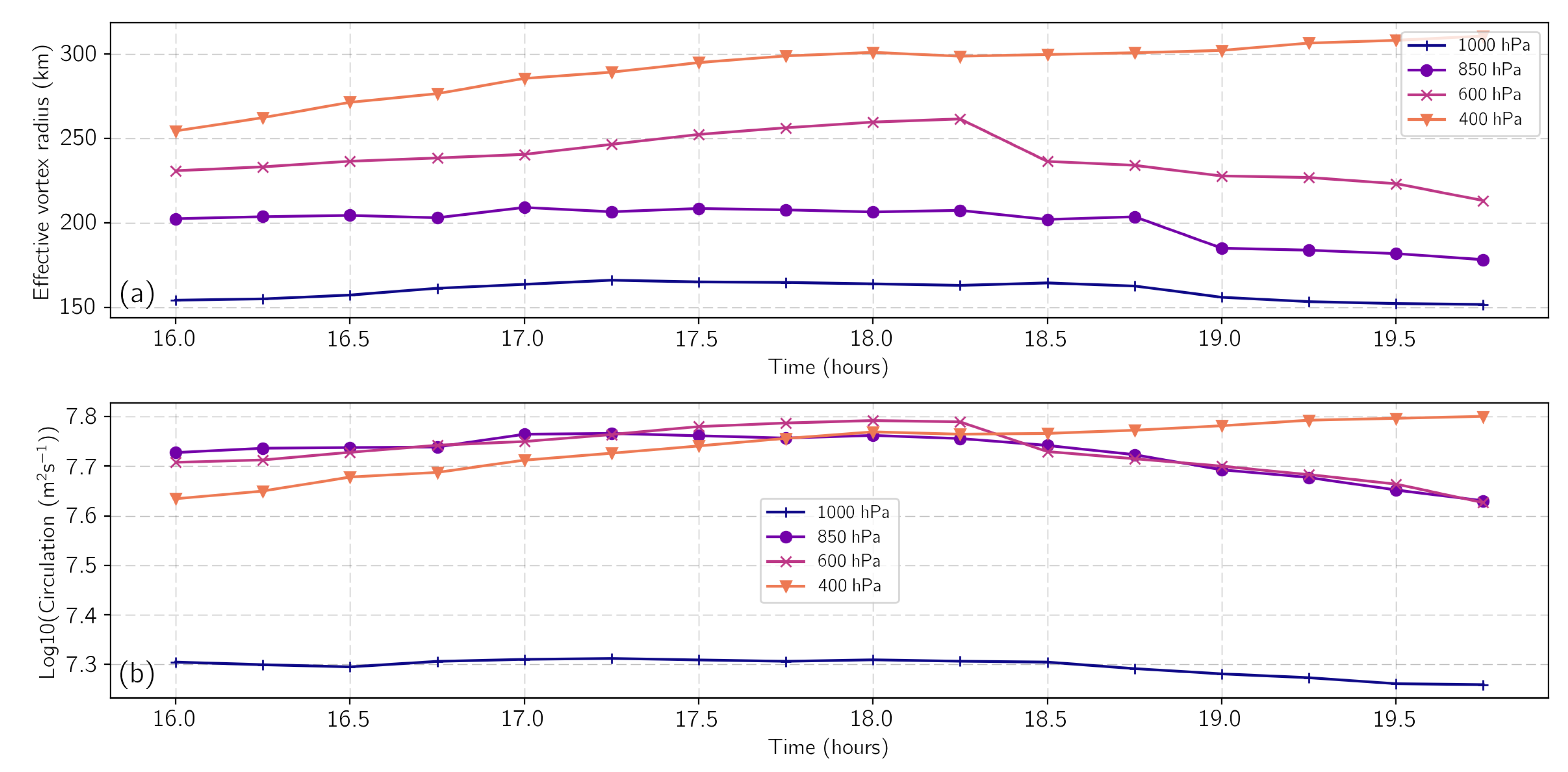
Figure 4.
Properties of Kyrill over its lifetime derived from six-hourly NCEP data at different height levels: (a) Effective radius (km) with area A and (b) circulation (ms).
Figure 4.
Properties of Kyrill over its lifetime derived from six-hourly NCEP data at different height levels: (a) Effective radius (km) with area A and (b) circulation (ms).

Figure 5.
Frequency distributions of vortex properties of cyclonically-rotating vortices identified in the Northern Hemisphere (≥25 N) during the period 15 January 2007 00 UTC–19 January 2007 18 UTC at 850 hPa in NCEP data. (a) Circulation (ms) and (b) mean vorticity (s) averaged over the identified vortex area (estimated by (15)).

Figure 6.
In NCEP data, identified cyclonically-rotating vortices in the Northern Hemisphere on 18 January 2007 18 UTC at 850 hPa. (a) Color shading indicates the magnitude of the circulation of the systems; (b) color shading corresponds to the mean vorticity averaged over the identified vortex areas (estimated by ). Black contours: geopotential height in 80-m intervals; the thick black line corresponds to the 1440-m contour, while the green arrow points to Kyrill.

Figure 7.
Vortex patches field at 850 hPa identified in Climate Forecast System Reanalysis (CFSR) data on 18 January 2007 at 13 UTC color shaded (a) by their circulation magnitude (logarithm of circulation, circulation has units of ms) and (b) by their mean vorticity (in s). Geopotential height given in 80-m intervals as black contours; the thick black contour is the 1440-m geopotential height contour; the approximate location of Kyrill is indicated by the green arrow.

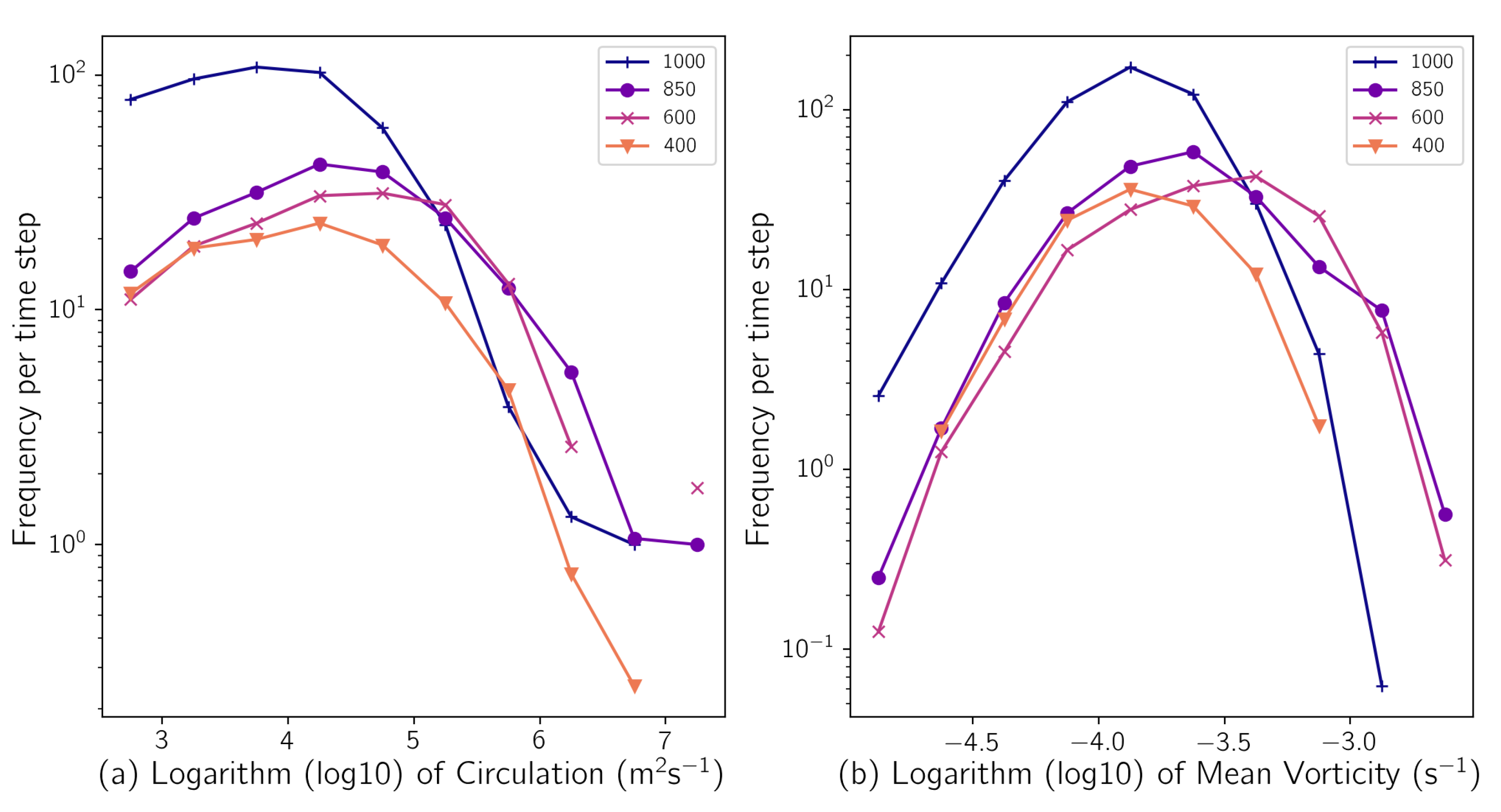
Figure 8.
Frequency-intensity distributions of (a) the logarithm of the circulation magnitude (ms) and (b) mean vorticity ( s) of vortices identified in CFSR data in the Northern Hemisphere (≥25 N) in the period between 17 January 2007 00 UTC and 19 January 2007 12 UTC (60 time steps). Frequencies are averaged over all time steps to derive a frequency per (one-hour) time step. Maximum values of Kyrill and their time of occurrence are indicated by the arrows and annotations.

Figure 9.
Vortices identified in CFSR data at 400 hPa for specific time steps color shaded (a–c) by their circulation magnitude (Log10(circulation (ms))) and (d–f) by their mean vorticity ( s). Only vortices are plotted that lie within the radius around Kyrill’s NCEP circulation center (green dot). The inner green circle represents the effective radius of Kyrill (as calculated in NCEP), and the outer green circle is given by the doubled effective radius. Black contours: geopotential height in 80-m intervals with the thick black contour equal to 7120 m.

Figure 10.
Vortices identified in CFSR data at 850 hPa for specific time steps color shaded (a–c) by their circulation magnitude (Log10(circulation (ms))) and (d–f) by their mean vorticity ( s). Other properties and contours as described in Figure 9, except the thick black contour, which is equal to a geopotential height of 1440 m.

Figure 11.
Three-dimensionally overlaid mean vorticity (in s) fields computed from CFSR data for different time steps. The domain moves and broadens with Kyrill’s circulation center and effective radius derived from NCEP data. Only vortices inside this effective radius are plotted.
Figure 11.
Three-dimensionally overlaid mean vorticity (in s) fields computed from CFSR data for different time steps. The domain moves and broadens with Kyrill’s circulation center and effective radius derived from NCEP data. Only vortices inside this effective radius are plotted.

Figure 12.
Temporal evolution of Kyrill’s vortex properties derived from CFSR data for 18 January 2007 (time in UTC) at different pressure levels inside a radius of 500 km around circulation center of Kyrill at 850 hPa: (a) effective radius (in km) and (b) logarithm of total circulation (in m s) derived by adding the positive circulations associated with Kyrill’s vortex structures.

Figure 13.
Frequency-intensity distributions per 15-min time steps of all vortex structures identified in the COSMO dataset that lie inside Kyrill’s NCEP radius for different height levels: (a) logarithm of circulation (ms) and (b) logarithm of the mean vorticity (s).
Figure 13.
Frequency-intensity distributions per 15-min time steps of all vortex structures identified in the COSMO dataset that lie inside Kyrill’s NCEP radius for different height levels: (a) logarithm of circulation (ms) and (b) logarithm of the mean vorticity (s).

Figure 14.
Temporal evolution of Kyrill’s vortex properties as seen in COSMO data for 18 January 2007 16:00 UTC–19:45 UTC (15-min time steps) at different pressure levels identified withhelp of the 2d -method with a threshold of 1.0: (a) effective radius (in km) and (b) logarithm of total circulation (in ms) derived by adding the positive circulations associated with Kyrill’s vortex structures.

Figure 15.
Vortex patches fields (a) derived by the two-dimensional -method and (b) derived by the three-dimensional -method, in the COSMO simulation on 18 January 2007 18:00 UTC color shaded by the logarithm of the mean vorticity (1/s) at 850 hPa. Black contours are the geopotential height in 80-m intervals; the thick black line corresponds to a geopotential height of 1320 m.

Figure 16.
Vortex patches fields derived by the two-dimensional -method in the COSMO simulation on 18 January 2007 18:00 UTC color shaded by the logarithm of the mean vorticity (1/s) (a) at 925 hPa and (b) at 700 hPa. Black contours are the geopotential height in 80-m intervals; the thick black line corresponds to a geopotential height of (a) 680 m and (b) 2800 m; the thick black circle in (a) highlights the position of a bookend vortex.


Table 1.
Summary of the data used to study Kyrill and the properties identified with the help of the -method. In the two higher resolved datasets, CFSR and COSMO, the sum of positive circulations was calculated inside the effective radius of Kyrill. This radius was derived from the NCEP data. The circulation and mean vorticity values are given for the 850-hPa level for the most intense periods of Kyrill.
| NCEP/DOE | CFSR | COSMO-CLM | |
|---|---|---|---|
| Reanalysis 2 | Reanalysis | Simulation | |
| Horizontal grid spacing | 2.5 (≈250 km) | 0.5 (≈50 km) | ≈2.8 km |
| Temporal resolution | 6 h | 1 h | 15 min |
| Investigated regions | Northern Hemisphere | Northern Hemisphere | Germany and Adjacent countries |
| (Sum of) Pos.circulation(s) | |||
| Maximum of mean vorticity |
© 2019 by the authors. Licensee MDPI, Basel, Switzerland. This article is an open access article distributed under the terms and conditions of the Creative Commons Attribution (CC BY) license (http://creativecommons.org/licenses/by/4.0/).
Share and Cite
MDPI and ACS Style
Schielicke, L.; Gatzen, C.P.; Ludwig, P. Vortex Identification across Different Scales. Atmosphere 2019, 10, 518. https://doi.org/10.3390/atmos10090518
AMA Style
Schielicke L, Gatzen CP, Ludwig P. Vortex Identification across Different Scales. Atmosphere. 2019; 10(9):518. https://doi.org/10.3390/atmos10090518
Chicago/Turabian StyleSchielicke, Lisa, Christoph Peter Gatzen, and Patrick Ludwig. 2019. "Vortex Identification across Different Scales" Atmosphere 10, no. 9: 518. https://doi.org/10.3390/atmos10090518
Note that from the first issue of 2016, this journal uses article numbers instead of page numbers. See further details here.