Use of Low-Cost Ambient Particulate Sensors in Nablus, Palestine with Application to the Assessment of Regional Dust Storms


1
Department of Civil Engineering, An-Najah National University, Nablus 44830, Palestine
2
Utah Water Research Laboratory, Department of Civil and Environmental Engineering, Utah State University, Logan, UT 84322, USA
*
Author to whom correspondence should be addressed.
Atmosphere 2019, 10(9), 539; https://doi.org/10.3390/atmos10090539
Submission received: 23 June 2019
/
Revised: 28 August 2019
/
Accepted: 5 September 2019
/
Published: 11 September 2019
(This article belongs to the Special Issue Ambient Aerosol Measurements in Different Environments)
Abstract
:Few air pollutant studies within the Palestinian territories have been reported in the literature. In March–April and May–June of 2018, three low-cost, locally calibrated particulate monitors (AirU’s) were deployed at different elevations and source areas throughout the city of Nablus in Northern West Bank, Palestine. During each of the three-week periods, high but site-to-site similar particulate matter less than 2.5 µm in aerodynamic diameter (PM2.5) and less than 10 µm (PM10) concentrations were observed. The PM2.5 concentrations at the three sampling locations and during both sampling periods averaged 38.2 ± 3.6 µg/m3, well above the World Health Organization’s (WHO) 24 h guidelines. Likewise, the PM10 concentrations exceeded or were just below the WHO’s 24 h guidelines, averaging 48.5 ± 4.3 µg/m3. During both periods, short episodes were identified in which the particulate levels at all three sites increased substantially (≈2×) above the regional baseline. Air mass back trajectory analyses using U.S. National Oceanic and Atmospheric Administration’s (NOAA) Hybrid Single-Particle Lagrangian Integrated Trajectory (HYSPLIT) model suggested that, during these peak episodes, the arriving air masses spent recent days over desert areas (e.g., the Saharan Desert in North Africa). On days with regionally low PM2.5 concentrations (≈20 µg/m3), back trajectory analysis showed that air masses were directed in from the Mediterranean Sea area. Further, the lower elevation (downtown) site often recorded markedly higher particulate levels than the valley wall sites. This would suggest locally derived particulate sources are significant and may be beneficial in the identification of potential remediation options.
1. Introduction
Airborne particulate matter (PM) is believed to have great influence on human health risks. PM refers to small particles suspended in the ambient air. PM10 refers to particles less than 10 µm in aerodynamic diameter, while PM2.5 refers to particles less than 2.5 µm in aerodynamic diameter [1]. As summarized by Lippmann et al. [2], PM10 represents the particulate fraction that can be inhaled via the body’s respiratory mechanisms, while the fraction referred to as PM2.5 is the subset that can remain within the system’s air flow pathway and potentially be deposited within the lungs’ oxygen exchange region (e.g., aveoli). Lelieveld et al. [3] estimated that PM (mostly PM2.5) pollution contributes to approximately 3.3 million premature deaths per year worldwide. Furthermore, this number is estimated to reach 6 million in the year 2050. PM also can cause acute asthma exacerbation, increased hospital admissions and emergency room visits, and decreased lung function [4,5]. Sources of PM could be manmade or natural. Manmade sources of PM include general combustion, vehicle emissions, and tobacco smoke. Natural sources include volcanoes, fires, dust storms, and aerosolized sea salt [6]. The World Health Organization (WHO) air quality guidelines [7] state that concentrations of PM2.5 should be less than 10 µg/m3 (annual average) and 25 µg/m3 (24 h average), whereas PM10 concentrations should be less than 20 µg/m3 (annual average) and 50 µg/m3 (24 h average).
As with any metropolitan area, the city of Nablus in Northern West Bank, Palestine (population 186,000 [8]) (see Figure 1a), contains numerous potential sources of particulate matter. These sources include transportation, quarry and stone cutting operations, industrial/commercial activities, and seasonal dust storms. However, few air pollutant studies within Palestine have been reported in the literature. Jodeh et al. [9] found that the annual average concentrations of PM10 and PM2.5 in the city of Nablus were approximately 160 μg/m3 and 111 μg/m3, respectively—approximately an order of magnitude above the WHO guidelines. Although they sampled at eight rotating locations and for a full year period, neither the effect of elevation nor the potential dust storms were examined. Abdeen el al. [10] showed that the annual PM2.5 concentrations in the city of Nablus were above the WHO guidelines and also above the average annual concentrations in 11 other cities in Palestine, Jordan, and Israel (30.9 µg/m3 compared to 28.7 µg/m3); however their reported values were around three times lower than those reported by Jodeh et al. [9]. Abdeen et al. [10] also showed that, in general, organic matter comprised about 50% of PM2.5 and that dust storms have great impact on the spring season concentrations. Although these findings are important for comparisons between Nablus and other cities in the region, they do not indicate the spatial variability of PM concentrations in the city, nor the origin of these particles. Despite the lack of studies to date that have investigated the impact of air pollution on the human health of the residents of the city, Sayara et al. showed that PM from quarries near the city of Nablus have negatively affected agriculture and plant biodiversity [11].
In Northern Palestine, including the city of Nablus, dust storms generally occur in the spring season [12]. These dust storms usually obstruct visibility (Figure 2), reduce soil fertility, limit solar radiation, cause radio communication problems and local climate effects, deposit salt, contaminate drinking water, disrupt power supplies, and transmit diseases in humans, plants, and animals [13,14]. Previous studies in the Middle East and Southeastern Europe have recorded significant dust load, originating mainly from the Sahara and the Arabian Peninsula [15,16,17].
To assess the air quality in the city of Nablus during and outside of dust storms, we measured real-time PM concentrations using low-cost AirU sensors (AirUs). In addition to their affordable cost, these sensors can provide real-time, high spatial resolution measurements in very compact, user-friendly platforms [19]. The development of such sensors can be an important evolution in the improvement of temporal and spatial air quality assessments and, ultimately, lead to better quantification of exposure to local air pollutants [20]. However, the data obtained by these sensors are of questionable accuracy [19,21]. To address concerns of demonstrated low accuracy, the data from these sensors can be validated against data from reference instruments [21]. Previous studies have shown that these sensors, when properly calibrated, can generate data comparable to data generated from much more expensive reference instruments [19,20,21,22,23,24].
Long-range transport models, such as the U.S. National Oceanic and Atmospheric Administration’s Hybrid Single-Particle Lagrangian Integrated Trajectory model (NOAA-HYSPLIT) [25,26], are additional resources that can be used to track the impact of air masses of different regional exposures on a given area. NOAA-HYSPLIT has been used for trajectory analysis to track the origins of air masses and understand the spatial and temporal variability of aerosol concentrations [27]. It is also useful in tracking air masses and analyzing dominant transport patterns leading to air pollution episodes [28].
As an extension to the findings of the previously cited studies [9,10] concerning the city of Nablus and the region’s air quality, this paper examines the concentrations of PM10 and PM2.5 at three different locations in the city of Nablus that represent different elevations and potential pollution sources. The measurements were conducted using locally calibrated, low-cost PM sensors in two periods during March–April and May–June of 2018. The study also uses back trajectory analysis using NOAA-HYSPLIT to assess the origin and transport of aerosols found in the ambient air in the city of Nablus during these two periods.
2. Methodology
2.1. Study Area and Site Selection
The city of Nablus (Figure 1b) is located in a valley between two mountains: Ebal to the north and Jerzim to the south, with an altitude ranging from 550 m to about 900 m above sea level (ASL). The city is located in a Mediterranean climate of hot, dry summers and cool, rainy winters. The hottest months in Nablus are typically July and August, with an average high temperature of 28.9 °C. The coldest month is usually January, with an average low of 3.9 °C [29].
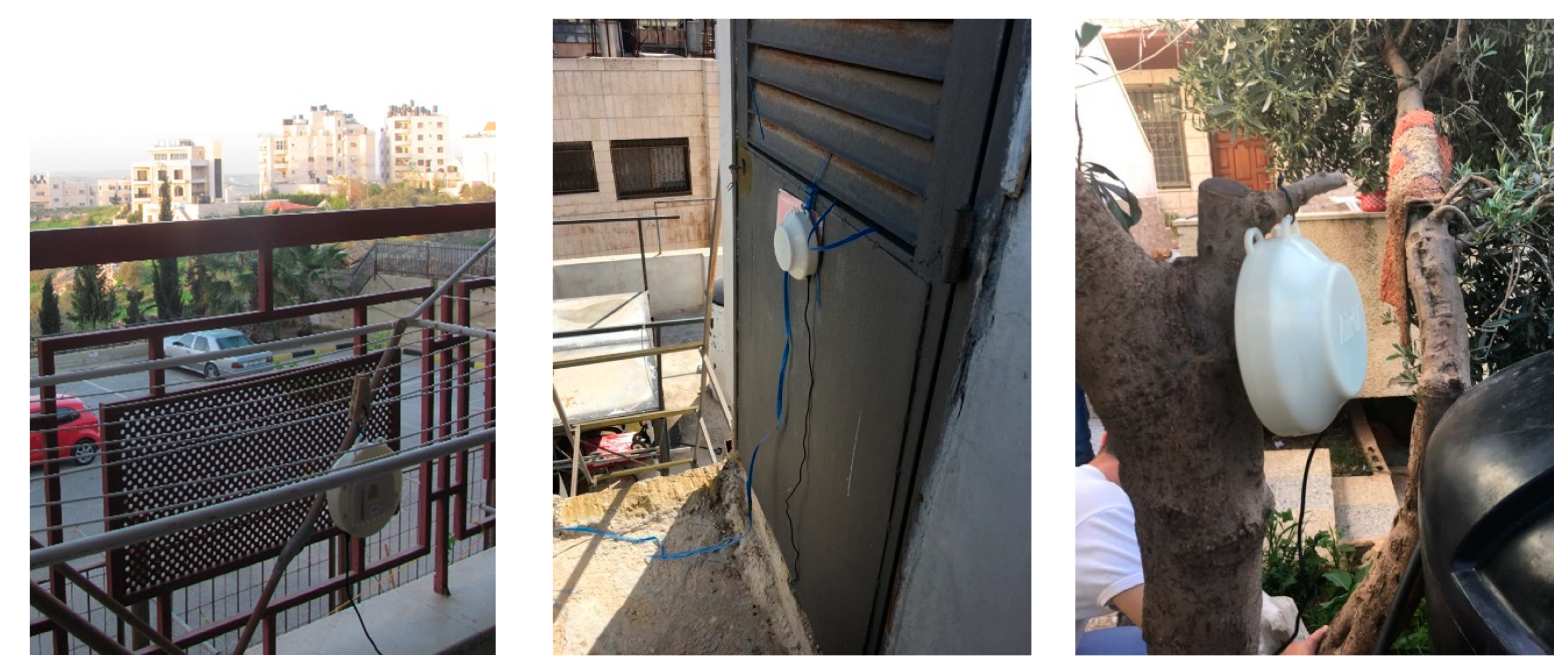
To examine the spatial and temporal distribution of PM concentrations in the city of Nablus, three sites were selected at different elevations and differing local source areas throughout the city (Figure 1b). The first site (SW) was located at an apartment complex on the southwest wall of the Nablus valley (687 m ASL). The second site (DT) was located near the downtown area and near the valley bottom (482 m ASL). The third site (NE) was located at a private residence on the northeast side of the Nablus valley (626 m ASL). The sensors collected data in 2018 from March to April and May to June. Figure 3 shows the sensors at the three sampling locations.
2.2. Calibration of Low-Cost PM Sensors
In recent years, low-cost PM and gaseous pollutant sensors have become widely available. As summarized by Kuula et al. [30], most of the commercially available, low-cost particulate systems operate by passing a particulate-laden stream through a collimated light beam, typically an infrared LED. Any scattered light is detected by an appropriate photodiode stationed at a right angle to the original beam, creating an increased electrical signal relative to the characteristics of the introduced particulate material. As potential particulate composition, shape, and size distributions can be expected to absorb and scatter the incident light differently, it is critical that such low-cost sensors be calibrated to local particulate conditions [19,20,23,31]. The World Air Quality Project [32] has compiled a partial list of many base low-cost, particulate sensors.
In this study, three low-cost monitoring devices (AirUs) that utilize Plantower Particulate Matter Sensor (PMS) 3003 sensors were deployed. The AirUs were developed by the University of Utah’s College of Engineering [31,33]. Becnel et al. [34] explicitly describes the AirU systems, but in brief, these systems are integrated measurement platforms that incorporate the listed particulate sensor with on-board data acquisition and networking capabilities and support measurement of other relevant parameters such as GPS location, ambient temperature, relative humidity, and specific pollutant gas detection (nitric oxide and carbon monoxide). One-minute averaged data are stored internally on a micro SD card for post experiment recovery and analysis.
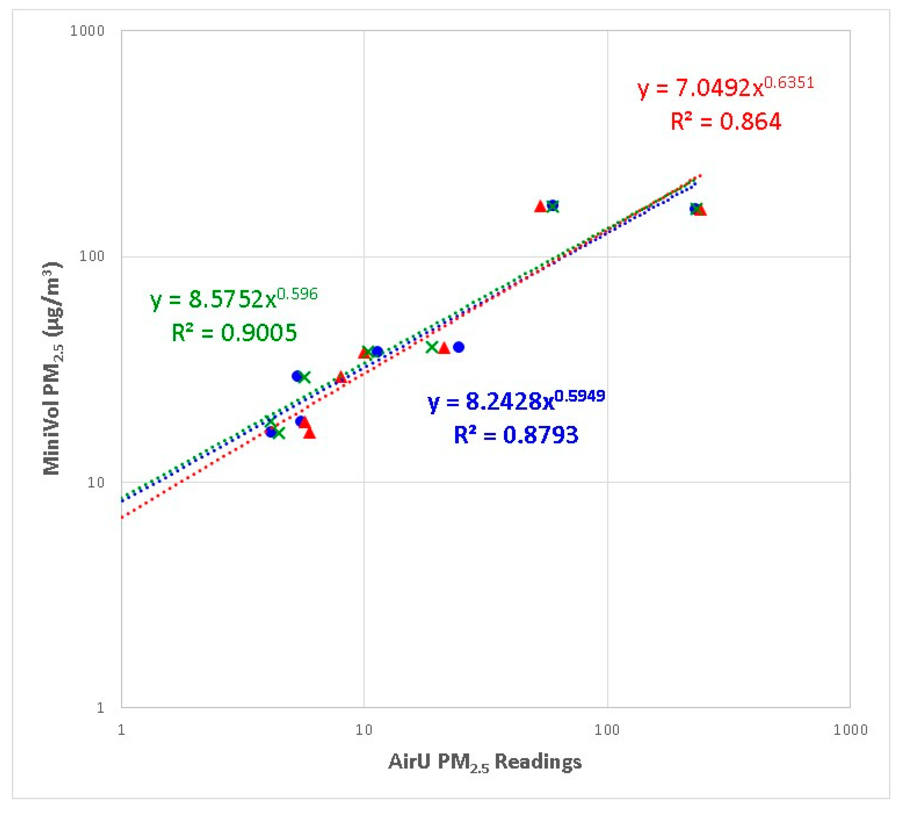
The AirUs were calibrated for local PM using a Mini-Vol configured for PM2.5 collection. The Mini-Vol is a filter-based, low-volume air sampler (Airmetrics Co., Inc.; 5 L/min flow rate). The instruments were collocated and operated for seven periods under differing ambient conditions. As the expected concentration range and particle composition across the chosen sample locations was unknown, the researchers judged it best to calibrate the sensors across differing local PM types. The periods ranged from one day to several days depending on the expected PM concentrations, during which the PM2.5 ranged from approximately 17 to 168 µg/m3. The runs were performed in several locations: on a university campus (in the Water and Environmental Studies Institute—WESI), at an apartment complex (at SW location), and at a smoke shop/coffee house. During each run, the Mini-Vol collected the PM2.5 onto a pre-weighed 47 mm Teflon filter and the AirUs recorded the near-real-time, 1-min averaged apparent PM concentrations. After each run, the total Mini-Vol sample volumes were noted and differences between the pre- and post-filter weights were used to determine the true ambient PM2.5 concentrations. Similar to standard PM2.5 filter protocols, when filters were not deployed, they were housed in uniquely marked, separate petri dishes and stored at room temperature in a silica gel-based desiccator. The pre- and post-filter weights were determined by multiple, once-per-day weighing on a balance capable of 10 µg resolution until a standard deviation of 20 µg was attained. The mass differentials found by the Mini-Vols across all the calibration runs ranged from 140 µg to 400 µg. Using the stated standard deviation limit of 20 µ, the mass-related uncertainty ranged from 5.7 to 14.3%, with an average of 9.4 ± 2.4% at the 95% confidence interval.
The average concentrations from the AirUs during each of the runs were compiled from the recorded data. Figure 4 compares the PM2.5 calibration results for the three AirUs to the Mini-Vol concentrations. AQ-SPEC [35] and Bulot et al. [36] have shown that systems based on the Plantower family of sensors (1003, 3003, 5003, 7003), which differ primarily by specific utilized wavelengths and internal flow paths, can all achieve high to moderate linear correlations compared to certified field data, having good precision but low accuracy. Further, as Kelly et al. [31] specifically showed, when the linearity of the AirU systems shifted above 40 µg/m3, a more reflective power curve fit was applied to the data obtained within this study. The manufacture’s literature suggests that changes in ambient temperature and relative humidity may have a significant effect of the accuracy and precision of these low-cost, light scattering-based sensors. However, as cited in the available literature, field evaluations have shown reported readings to be statistically impacted only when the relative humidity was >75%. The impacts from changes in temperature alone were negligible [35,37,38]. According to the Palestinian Meteorological Department [29], relative humidity in Nablus ranges from 51% to 62% for the period March to June, thus, potential humidity effects were also ignored.
Owing to system and time limitations, PM10 was not calibrated directly through the Mini-Vol filters, but rather was calculated by multiplying the apparent PM10 from the AirUs with the ratio of calibrated-to-apparent PM2.5 concentrations. Although not ideal, this approach should be indicative enough in this application given that Sayahi et al. [33] showed similar proportionality constants (linear calibration slope terms) for PM2.5 and PM10 concentrations for multiple PMS 1003 and 5003 sensors when compared to collocated, certified (e.g., EPA) monitors in northern Utah, USA. However, during the spring and under wildfire episodes, as reported by Sayahi et al., the PM10 readings were less well correlated when compared with the regulatory monitors than PM2.5 readings and the slope terms did diverge.
2.3. Back Trajectory Analysis Using NOAA-HYSPLIT
As a verification of when the Nablus airshed may be potentially impacted by regional dust events, back trajectory analyses were conducted using the NOAA-HYSPLIT on-line modeling protocols [25,26]. The available HYSPLIT was executed multiple times for targeted arrival times in Nablus relative to changes in observed PM concentrations. The PM time series data collected during this study were examined for periods when concentrations appeared to be representative of average conditions and for short periods of time when concentrations appeared to be impacted by events such as regional dust storms. The model was operated in “normal trajectory” mode, with 100 m Above Ground Level (AGL) arrival heights, and multiple arrival time differentials varying from six to twelve hours. The specific arrival location was 32.25520° N and 35.25070° E, approximately central to the Nablus region. Finally, to gain confidence is the modeled trajectories, replicate analyses were performed for the target time periods using three different available global meteorological data sets (GDAS 1 (GDAS), GDAS 0.5 (GFSG), and REANALYSIS (CDC1)).
3. Results and Discussion
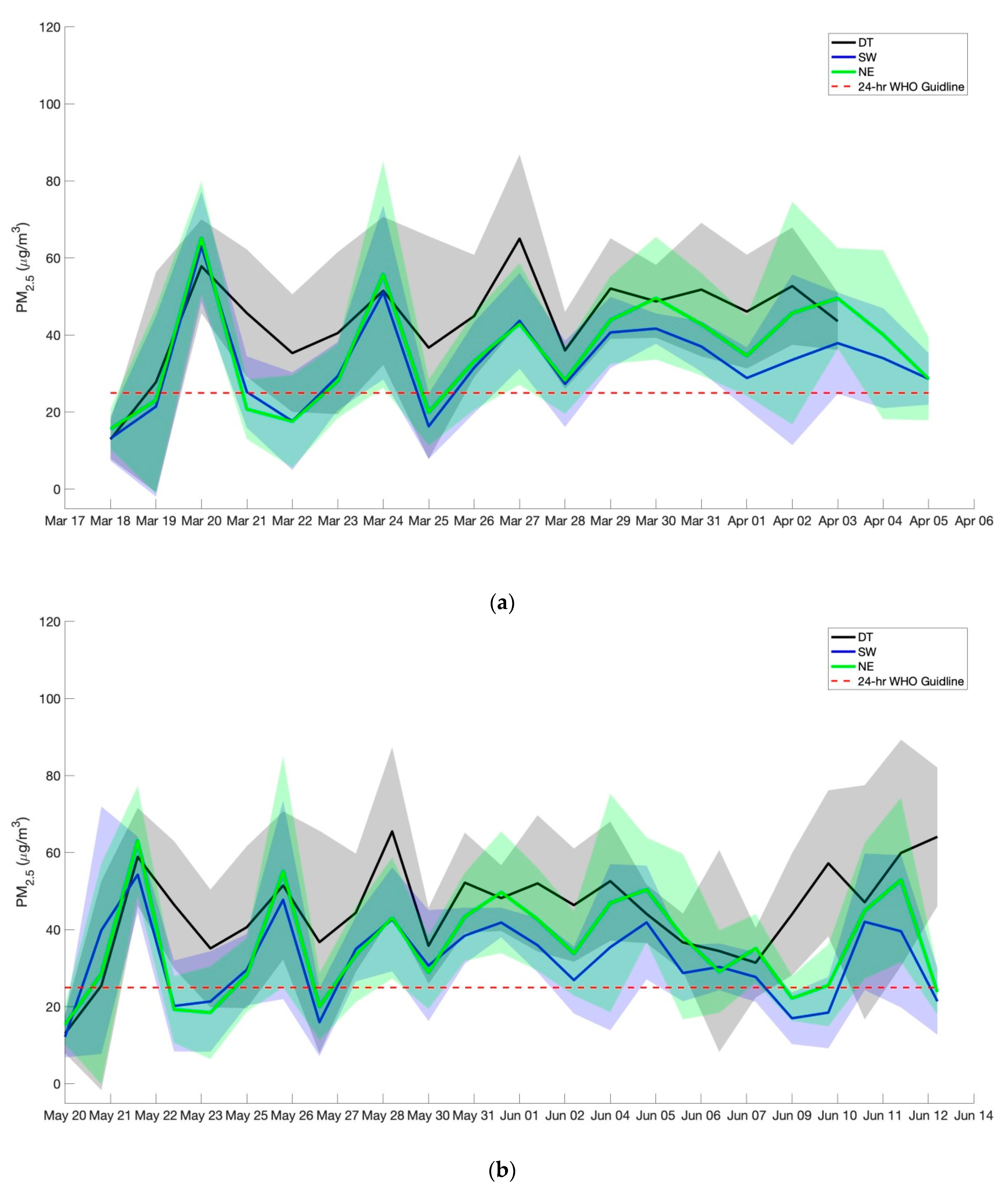
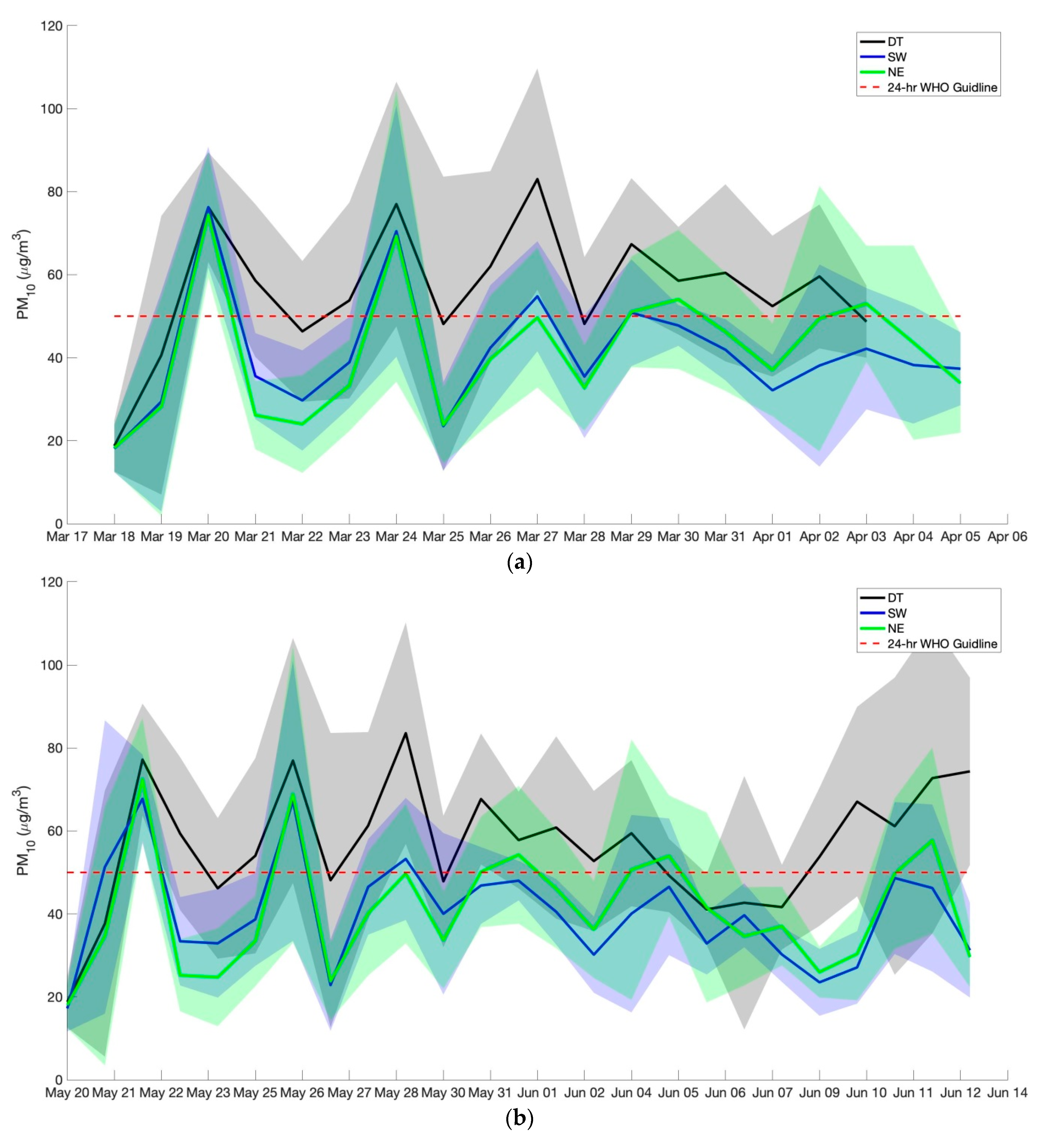
The calibrated AirUs were deployed to the three sampling locations for two periods. The first period spanned from 18 March 2018 to 5 April 2018, while the second period spanned from 20 May 2018 to 13 June 2018. Figure 5 shows the daily averages (the AirUs were programmed for one minute averages) of the PM2.5 concentrations from each of the three sites during the two periods, and Figure 6 shows those daily averages for PM10 concentrations for the same sites during the same periods. As shown in both figures, the PM concentrations were found to be highly variable and exceeded the WHO guidelines most of the time.
Table 1 shows the average, maximum, and minimum PM values (in µg/m3) in the three sampling locations during the two sampling periods. It also shows that the average daily PM2.5 concentrations during both periods, and in all locations, exceeded the WHO guidelines (25 µg/m3 24 h) 72% to 96% of the time. The overall average PM2.5 concentration in the three locations for both periods, which may be viewed as the average PM2.5 concentration for the Nablus area, was calculated to be 38.2 ± 3.6 µg/m3. This average PM2.5 concentration is very similar to the values reported by Abdeen et al. [10] and similarly lower than the values of Johet et al. [9].
For PM10, the average daily concentrations were found to exceed the WHO guideline (50 µg/m3 24 h) at the DT location 64% of the time, and 15% to 28% of the time at the other two locations. The site-to-site average values show that PM2.5 made up approximately 76.4%, 75.7%, and 84.9% of the PM10 at the DT, SW, and NE sites, respectively. These numbers suggest that the majority of PM pollution is composed of fine particles smaller than 2.5 µm. As can also be derived from Table 1, the PM2.5-to-PM10 ratios do not seem to vary substantially from the observed average values to the maximum concentrations, which are likely enhanced by the long-range transport of desert dusts. Conversely, Jaafari et al. [39] have shown noticeable decreases in the PM2.5-to-PM10 ratios when areas are suspected or known to be impacted by regional or local dust storms. Desert dust size distributions are generally reported to be dominated by coarse particle sizes (>10 µm), but the coarser particle sizes may be selectively removed as an elevated dust plume is transported long-range downwind, resulting in evolving size distributions dominated by smaller particles [40,41]. Overall average PM10 concentration from the three locations for both periods was 48.5 ± 4.3 µg/m3, which is just below the 24 h WHO guideline.
As previously indicated, both the PM2.5 and the PM10 concentrations at the DT location were significantly higher (approximately 33% and 37%, respectively) than the other two locations (SW and NE) during both periods. Tukey’s test was performed, and the results show that p-values for the hypothesis that the mean differences (DT–SW and DT–NE) were equal to zero were both very small (approximately 9.5 × 10⁻¹⁰). This indicates the significant difference between the concentrations at the DT location and other two locations.
There are many possible reasons for these higher concentrations, and more detailed apportionment studies would have to be performed to be certain. However, anecdotally, the DT location is closer to more suspected pollutant sources (shopping/market areas, major roadways/highways, industrial activities, and public areas). It is also lower in valley floor and may be more susceptible to drainage flows and capping inversions, which may concentrate and trap PM and other pollutants.
A closer look at PM2.5 and PM10 concentration time series (Figure 5 and Figure 6) revealed periods where the PM concentrations were high at all three sites, such as the spikes on March 24. On the other hand, there were also periods wherein the PM concentrations at the DT site spiked up but those at the SW and NE sites did not, as observed on March 21. The episodic higher concentration spikes at all locations could possibly be attributed to the occurrence of seasonal dust storms. To test this hypothesis, the NOAA-HYSPLIT model was used to model the predicted origins of air masses during these periods. Figure 7a shows the three-day back trajectories for arrival times (Δt = 6 h) on March 23–24 using the three available meteorological datasets. These trajectories were relatively similar across the three datasets; however, the finer resolved and updated meteorological dataset (REANALYSIS (CDC1)) predicted a more long-range, rotational trajectory for the morning (6:00 local, green trajectory as seen in Figure 7a) on March 24. In general, the trajectories arriving on March 23 through that midnight showed slow moving air masses, with a more rapidly moving anticyclonic (high pressure) flow in the morning hours of March 24. The subsequent trajectories throughout the day on March 24 consistently showed rapid moving air masses traveling along the north edge of the African continent.
As shown in Figure 7b,c, prior to the westward shift in the back trajectories, the PM2.5 and PM10 concentrations remained relatively low and consistent at the SW and NE sites, while the DT site routinely showed excursions two-to-three times the levels at the other sites. The frequent increases unique to the DT site are consistent with significant impacts from local sources. During the period of the westward, fast moving trajectories (March 24), the PM concentrations at all of the observed sites tracked each other well and suggested a common, region-wide source (e.g., long-range dust transport). Meteorological observations near the Ben Gurion Airport (about 40 km southwest of Nablus) support the passage of a regional high pressure system during the same time period, and the archived meteorological data file also noted periods of atypical haze and dust similar to the high PM periods observed in Nablus [42]. Furthermore, these results are consistent with results from previous studies in the region in terms of origin, added PM concentrations, and time of the year in which these dust storms typically occur [14,15,16].
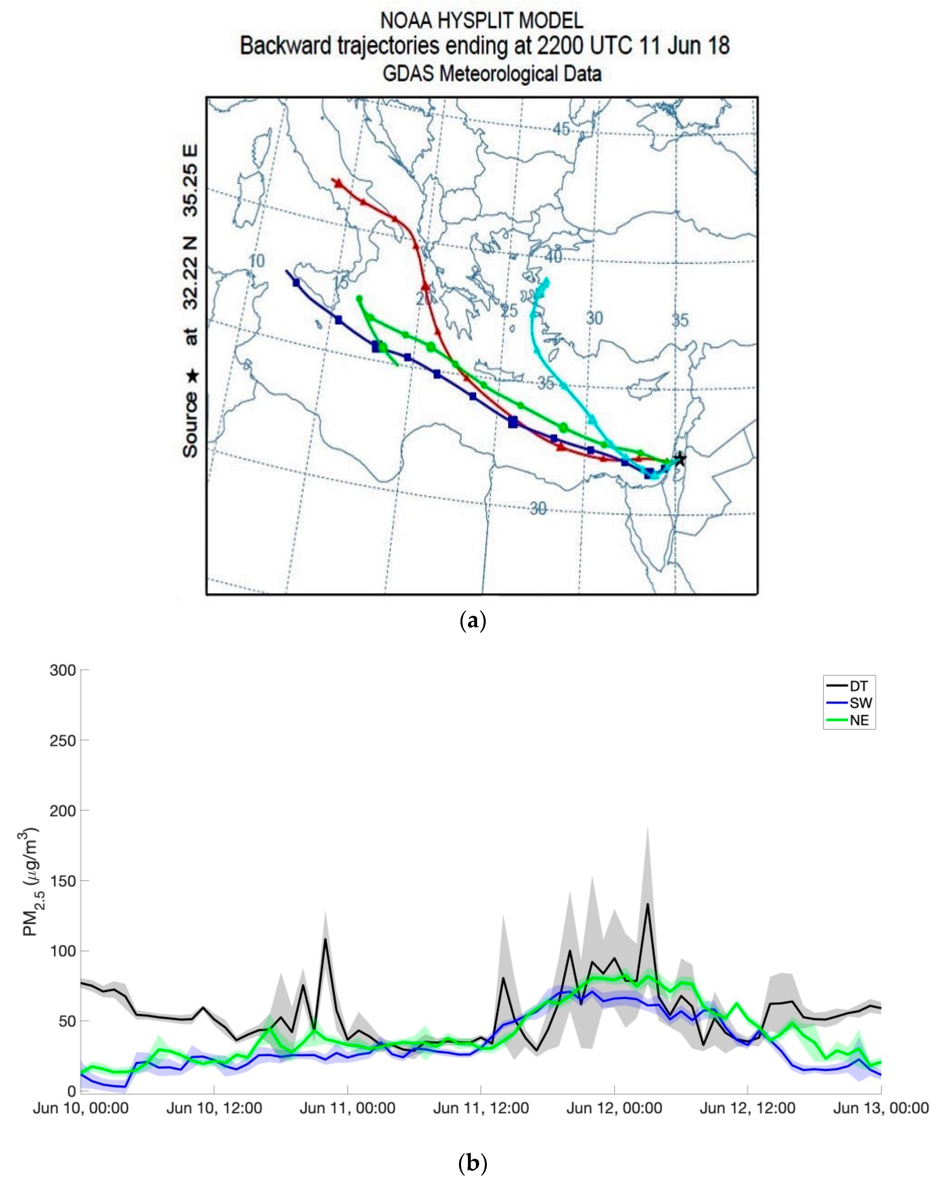
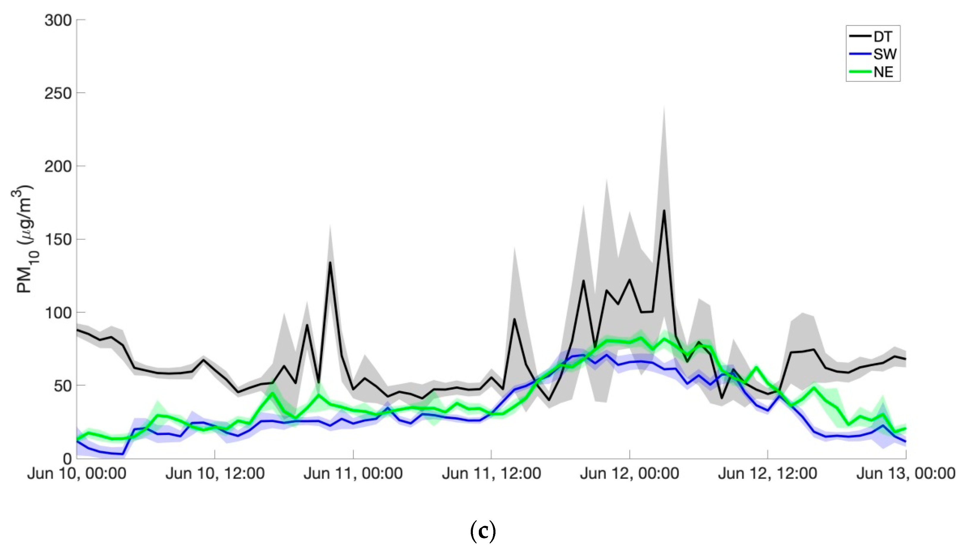
The NOAA-HYSPLIT model was used again to track the origins of air masses during two days in the May–June period (10–12 June), this time examining a period wherein the observed PM2.5 concentrations started at the relatively low level of around 20 µg/m3. The model was executed with the same three meteorological datasets as the previous examination, but the separate modeling runs did not result in significantly different back trajectories. Figure 8 shows the three-day back trajectories using the 1° resolution GDAS meteorological dataset and, as can be seen, the air masses came mostly from the relatively clean Mediterranean region. Once again, higher PM excursions were observed most regularly at the DT site, particularly during the late night of 10 June and early morning of 11 June (Figure 8). Further, all three locations showed a general increase in PM concentrations centered around midnight on 12 June, when back trajectory analysis suggested that the air mass spent time over the Italy/Greece regions. However, the measurements at the DT site, most notably PM10, once again showed more temporal variability and elevated concentrations than the other two sites. Similar to the March–April period (Figure 7), these DT localized spikes are most likely attributed to nearby emissions.
4. Conclusions and Recommendations
In this study, three locally calibrated low-cost PM sensors (AirUs) were used to measure PM2.5 and PM10 concentrations in three different locations in the city of Nablus during March–April and May–June of 2018. Furthermore, the NOAA-HYSPLIT model was used to assess one of the potential sources of PM pollution in the city of Nablus, which is the occurrence of seasonal dust storms.
The results show that there is a significant PM problem in the city of Nablus, where average concentrations almost daily exceeded the 24 h WHO guidelines for both PM2.5 and PM10. In summary, the overall average for PM2.5 in the Nablus region was 38.2 ± 3.6 µg/m3, while the overall PM10 averaged 48.5 ± 4.3 µg/m3. These daily averages are very similar to a regional study reported by Abdeen et al. [10], but are approximately three times lower than those reported by Jodeh et al. [9]. The results also showed that the PM2.5 and PM10 concentrations were often two to three times higher at the DT location compared to the other sampling sites. The DT location is lower in elevation and closer to more suspected pollutant sources. In addition, the occurrence of dust storms, especially in March–April, were found to exacerbate the pollutant concentrations by transporting large amounts of PM from neighboring regions.
The success of the local calibration and deployment of the low-cost particulate sensors in characterizing the PM2.5 and PM10 concentrations in Nablus, Palestine, puts forth an efficient and effective methodology for area-wide pollutant studies. Further studies in the Nablus region, and in similar regions, using a denser sensor network could be performed to identify more area-specific pollutant levels, local source strengths, and possible remediation recommendations.
Author Contributions
Conceptualization, A.K. and R.S.M.; methodology, R.S.M.; software, A.K.; validation, A.K. and R.S.M.; formal analysis, A.K. and R.S.M.; investigation, A.K. and R.S.M.; resources, R.S.M.; data curation, A.K.; writing—original draft preparation, A.K.; writing—review and editing, A.K. and R.S.M.; visualization, A.K.; supervision, R.S.M.; project administration, A.K. and R.S.M.; funding acquisition, A.K. and R.S.M.
Funding
This research was financially funded by An-Najah National University research fund No. ANNU-1819-Sc15. Martin’s participation was made possible through the U.S. Fulbright Foundation as a Visiting Scholar. Further, the Utah Water Research Laboratory and Martin provided donations and/or equipment, which were used during the study.
Acknowledgments
The Authors are thankful to Eng. Hanan Ja’far for helping in the calibration process. Many thanks to Zuhdi Iskandar and Ahmad Ayyad for providing access to sampling sites.
Conflicts of Interest
The authors declare no conflict of interest.
References
- Davidson, C.I.; Phalen, R.F.; Solomon, P.A. Airborne Particulate Matter and Human Health: A Review. Aerosol Sci. Technol. 2005, 39, 737–749. [Google Scholar] [CrossRef]
- Lippmann, M.; Yeates, D.B.; Albert, R.E. Deposition and clearance of inhaled particles. Br. J. Ind. Med. 1980, 37, 337–362. [Google Scholar] [PubMed]
- Lelieveld, J.; Evans, J.S.; Fnais, M.; Giannadaki, D.; Pozzer, A. The contribution of outdoor air pollution sources to premature mortality on a global scale. Nature 2015, 525, 367–371. [Google Scholar] [CrossRef] [PubMed]
- Li, N.; Hao, M.; Phalen, R.F.; Hinds, W.C.; Nel, A.E. Particulate air pollutants and asthma: A paradigm for the role of oxidative stress in PM-induced adverse health effects. Clin. Immunol. 2003, 109, 250–265. [Google Scholar] [CrossRef]
- Kim, K.-H.; Kabir, E.; Kabir, S. A review on the human health impact of airborne particulate matter. Environ. Int. 2015, 74, 136–143. [Google Scholar] [CrossRef]
- Anderson, J.O.; Thundiyil, J.G.; Stolbach, A. Clearing the Air: A Review of the Effects of Particulate Matter Air Pollution on Human Health. J. Med. Toxicol. 2012, 8, 166–175. [Google Scholar] [CrossRef] [PubMed]
- Krzyzanowski, M.; Cohen, A. Update of WHO air quality guidelines. Air Qual. Atmos. Heal. 2008, 1, 7–13. [Google Scholar] [CrossRef] [Green Version]
- PCBS. Preliminary Results of the Population, Housing and Establishments Census, 2017. 2018. Available online: http://www.pcbs.gov.ps/portals/_pcbs/PressRelease/Press_En_Preliminary_Results_Report-en-with-tables.pdf (accessed on 7 September 2019).
- Jodeh, S.; Hasan, A.R.; Amarah, J.; Judeh, F.; Salghi, R.; Lgaz, H.; Jodeh, W. Indoor and outdoor air quality analysis for the city of Nablus in Palestine: Seasonal trends of PM10, PM5.0, PM2.5 and PM1.0 of residential homes. Air Qual. Atmos. Heal. 2017, 11, 229–237. [Google Scholar] [CrossRef]
- Abdeen, Z.; Qasrawi, R.; Heo, J.; Wu, B.; Shpund, J.; Vanger, A.; Sharf, G.; Moise, T.; Brenner, S.; Nassar, K.; et al. Spatial and temporal variation in fine particulate matter mass and chemical composition: The middle east consortium for aerosol research study. Sci. World J. 2014, 2014, 878704. [Google Scholar] [CrossRef]
- Sayara, T.; Hamdan, Y.; Basheer-salimia, R. Impact of Air Pollution from Quarrying and Stone Cutting Industries on Agriculture and Plant Biodiversity. Resour. Environ. 2016, 6, 122–126. [Google Scholar]
- Kutiel, H.; Furman, H. Dust Storms in the Middle East: Sources of Origin and their Temporal Characteristics. Indoor Built Environ. 2003, 12, 419–426. [Google Scholar]
- Middleton, N.J. Desert dust hazards: A global review. Aeolian Res. 2017, 24, 53–63. [Google Scholar] [CrossRef]
- Krasnov, H.; Katra, I.; Koutrakis, P.; Friger, M.D. Contribution of dust storms to PM10 levels in an urban arid environment. J. Air Waste Manag. Assoc. 2014, 64, 89–94. [Google Scholar] [CrossRef] [PubMed]
- Remoundaki, E.; Bourliva, A.; Kokkalis, P.; Mamouri, R.E.; Papayannis, A.; Grigoratos, T.; Samara, C.; Tsezos, M. PM10 composition during an intense Saharan dust transport event over Athens (Greece). Sci. Total Environ. 2011, 409, 4361–4372. [Google Scholar] [CrossRef] [PubMed]
- Torfstein, A.; Teutsch, N.; Tirosh, O.; Shaked, Y.; Rivlin, T.; Zipori, A.; Stein, M.; Lazar, B.; Erel, Y. Chemical characterization of atmospheric dust from a weekly time series in the north Red Sea between 2006 and 2010. Geochim. Cosmochim. Acta 2017, 211, 373–393. [Google Scholar] [CrossRef]
- GADM, Maps and Data. Available online: https://gadm.org (accessed on 7 September 2019).
- Ministry of Local Governance. GeoMOLG. Available online: geomolg.ps (accessed on 7 September 2019).
- Castell, N.; Dauge, F.R.; Schneider, P.; Vogt, M.; Lerner, U.; Fishbain, B.; Broday, D.; Bartonova, A. Can commercial low-cost sensor platforms contribute to air quality monitoring and exposure estimates? Environ. Int. 2017, 99, 293–302. [Google Scholar] [CrossRef] [PubMed]
- Thompson, J.E. Crowd-sourced air quality studies: A review of the literature & portable sensors. Trends Environ. Anal. Chem. 2016, 11, 23–34. [Google Scholar]
- Schneider, P.; Castell, N.; Vogt, M.; Dauge, F.R.; Lahoz, W.A.; Bartonova, A. Mapping urban air quality in near real-time using observations from low-cost sensors and model information. Environ. Int. 2017, 106, 234–247. [Google Scholar] [CrossRef] [PubMed]
- Holstius, D.M.; Pillarisetti, A.; Smith, K.R.; Seto, E. Field calibrations of a low-cost aerosol sensor at a regulatory monitoring site in California. Atmos. Meas. Tech. Discuss. 2014, 7, 605–632. [Google Scholar] [CrossRef]
- Spinelle, L.; Gerboles, M.; Villani, M.G.; Aleixandre, M.; Bonavitacola, F. Field calibration of a cluster of low-cost available sensors for air quality monitoring. Part A: Ozone and nitrogen dioxide. Sens. Actuators B Chem. 2015, 215, 249–257. [Google Scholar] [CrossRef]
- Mead, M.I.; Popoola, O.A.M.; Stewart, G.B.; Landshoff, P.; Calleja, M.; Hayes, M.; Baldovi, J.J.; McLeod, M.W.; Hodgson, T.F.; Dicks, J.; et al. The use of electrochemical sensors for monitoring urban air quality in low-cost, high-density networks. Atmos. Environ. 2013, 70, 186–203. [Google Scholar] [CrossRef] [Green Version]
- Draxler, R.R.; Hess, G.D. An Overview of the HYSPLIT_4 Modelling System for Trajectories, Dispersion, and Deposition. Aust. Meteorol. Mag. 1998, 47, 295–308. [Google Scholar]
- Stein, A.F.; Draxler, R.R.; Rolph, G.D.; Stunder, B.J.B.; Cohen, M.D.; Ngan, F. NOAA’s HYSPLIT Atmospheric Transport and Dispersion Modeling System. Bull. Am. Meteorol. Soc. 2015, 96, 2059–2077. [Google Scholar] [CrossRef]
- Alam, K.; Qureshi, S.; Blaschke, T. Monitoring spatio-temporal aerosol patterns over Pakistan based on MODIS, TOMS and MISR satellite data and a HYSPLIT model. Atmos. Environ. 2011, 45, 4641–4651. [Google Scholar] [CrossRef]
- Wang, F.; Chen, D.S.; Cheng, S.Y.; Li, J.B.; Li, M.J.; Ren, Z.H. Identification of regional atmospheric PM10 transport pathways using HYSPLIT, MM5-CMAQ and synoptic pressure pattern analysis. Environ. Model. Softw. 2010, 25, 927–934. [Google Scholar] [CrossRef]
- Palestinian Meteorological Department, PMD. Available online: http://pmd.ps (accessed on 7 September 2019).
- Kuula, J.; Mäkelä, T.; Hillamo, R.; Timonen, H. Response characterization of an inexpensive aerosol sensor. Sensors (Switzerland) 2017, 17, 12. [Google Scholar]
- Kelly, K.E.; Whitaker, J.; Petty, A.; Widmer, C.; Dybwad, A.; Sleeth, D.; Martin, R.; Butterfield, A. Ambient and laboratory evaluation of a low-cost particulate matter sensor. Environ. Pollut. 2017, 221, 491–500. [Google Scholar] [CrossRef] [PubMed]
- The Word Air Quality Project. Air Quality Monitoring Devices & Sensor Research. Available online: https://aqicn.org/sensor/ (accessed on 7 September 2019).
- Sayahi, T.; Butterfield, A.; Kelly, K.E. Long-term field evaluation of the Plantower PMS low-cost particulate matter sensors. Environ. Pollut. 2019, 245, 932–940. [Google Scholar] [CrossRef] [PubMed]
- Becnel, T.; Sayahi, T.; Le, K.; Goffin, P.; Butterfield, T.; Kelly, K.; Gaillardon, P.E. A distributed low-cost pollution monitoring platform. Internet Things J. 2018. [Google Scholar]
- AQ-SPEC. Field Evaluation Purple Air PM Sensor Background. 2017. Available online: http://www.aqmd.gov/aq-spec (accessed on 7 September 2019).
- Bulot, F.M.; Johnston, S.J.; Basford, P.J.; Easton, N.H.; Apetroaie-Cristea, M.; Foster, G.L.; Morris, A.K.; Cox, S.J.; Loxham, M. Long-term field comparison of multiple low-cost particulate matter sensors in an outdoor urban environment. Sci. Rep. 2019, 9, 1–13. [Google Scholar] [CrossRef] [PubMed]
- Williams, R.; Vallano, D.; Polidori, A.; Garvey, S. Spatial and Temporal Trends of Air Pollutants in the South Coast Basin Using Low Cost Sensors; U.S. Environmental Protection Agency: Washington, DC, USA, 2018; p. 9.
- Jayaratne, R.; Liu, X.; Thai, P.; Dunbabin, M.; Morawska, L. The influence of humidity on the performance of a low-cost air particle mass sensor and the effect of atmospheric fog. Atmos. Meas. Tech. 2018, 11, 4883–4890. [Google Scholar] [CrossRef] [Green Version]
- Jaafari, J.; Naddafi, K.; Yunesian, M.; Nabizadeh, R.; Hassanvand, M.S.; Ghozikali, M.G.; Nazmara, S.; Shamsollahi, H.R.; Yaghmaeian, K. Study of PM10, PM2.5, and PM1 levels in during dust storms and local air pollution events in urban and rural sites in Tehran. Hum. Ecol. Risk Assess. 2018, 24, 482–493. [Google Scholar] [CrossRef]
- Mahowald, N.; Albani, S.; Kok, J.F.; Engelstaeder, S.; Scanza, R.; Ward, D.S.; Flanner, M.G. The size distribution of desert dust aerosols and its impact on the Earth system. Aeolian Res. 2014, 15, 53–71. [Google Scholar] [CrossRef] [Green Version]
- Weinzierl, B.; Ansmann, A.; Prospero, J.M.; Althausen, D.; Benker, N.; Chouza, F.; Dollner, M.; Farrell, D.; Fomba, W.K.; Freudenthaler, V.; et al. The Saharan aerosol long-range transport and aerosol-cloud-interaction experiment: Overview and selected highlights. Bull. Am. Meteorol. Soc. 2017, 98, 1427–1451. [Google Scholar] [CrossRef]
- EuroWEATHER. Tel Aviv-BenGurion, Observed Conditions, Hourly Data. Available online: http://www.eurometeo.com/english/condition/city_LLBG/archive_select/meteo_Tel Aviv-Ben Gurion (accessed on 7 September 2019).
Figure 1.
(a) Location of the city of Nablus (country map source: [17]); (b) the locations of the sampling sites, the mountain summits, and the site where the pictures in Figure 2 were taken (aerial photograph, city boundary, road map, and building map source: [18]).

Figure 2.
The visibility in the city of Nablus: (a) during a dust storm in March 2014; (b) during a clear day in April 2014. The pictures were taken from a location southwest of the city (Figure 1b) facing northeast (Mount Ebal).
Figure 2.
The visibility in the city of Nablus: (a) during a dust storm in March 2014; (b) during a clear day in April 2014. The pictures were taken from a location southwest of the city (Figure 1b) facing northeast (Mount Ebal).

Figure 3.
The AirU sensors as deployed at the first (SW), second (DT), and third (NE) sites, respectively.
Figure 3.
The AirU sensors as deployed at the first (SW), second (DT), and third (NE) sites, respectively.

Figure 4.
Calibration results of the locally calibrated particulate monitors (AirUs) against the Mini-Vol. The different colors (and markers) represent different AirUs. The lowest MiniVol concentration was measured at the indoor (WESI) site, the middle 5 were measured at ambient sites, and the highest concentration was measured at a smoke shop (indoor site).

Figure 5.
Daily average of concentrations of particulate matter less than 2.5 µm in aerodynamic diameter (PM2.5) in the three locations—DT, SW, NE—compared to WHO guidelines (a) during the March–April period; (b) during the May–June period. (The shaded areas represent the standard deviations of the 1-min measurements in the 24 h period).

Figure 6.
Daily average of concentrations of particulate matter less than 2.5 µm in aerodynamic diameter (PM10) in the three locations—DT, SW, NE—compared to WHO guidelines (a) during the March–April period; (b) during the May–June period. (The shaded areas represent the standard deviations).
Figure 6.
Daily average of concentrations of particulate matter less than 2.5 µm in aerodynamic diameter (PM10) in the three locations—DT, SW, NE—compared to WHO guidelines (a) during the March–April period; (b) during the May–June period. (The shaded areas represent the standard deviations).

Figure 7.
Air mass trajectory and PM concentrations in the three locations during 23–25 March period (a) NOAA-HYSPLIT model results (GDAS—top, GFSG—middle, and CDC1—bottom). The colored lines represent the following arrival times: yellow—23 March at 12:00, magenta—23 March at 18:00, sky blue—24 March at 00:00, green—24 March at 06:00, blue—24 March at 12:00, and red—24 March at 18:00. The marks on the lines represent six-hour steps; (b) hourly PM2.5; (c) hourly PM10.


Figure 8.
Air mass trajectory and PM concentrations in the three locations during 10–13 June period (a) NOAA-HYSPLIT model results. The colored lines represent the following arrival times: sky blue—10 June at 12:00, green—11 June at 00:00, blue—11 June at 12:00, and red—12 June at 00:00; (b) hourly PM2.5; (c) hourly PM10.

Table 1.
Average, maximum, and minimum PM values (in µg/m3) in the three sampling locations, during the two sampling periods.
Table 1.
Average, maximum, and minimum PM values (in µg/m3) in the three sampling locations, during the two sampling periods.
| Location | March–April | |||||||
| PM2.5 | PM10 | |||||||
| Period Average | Max. Value + (Date/Time) | Min. Value + (Date/Time) | n/N $ | Period Average | Max. Value + (Date/Time) | Min. Value + (Date/Time) | n/N $ | |
| DT | 45.2 ± 3.5 * | 96.5 24 Mar/4am | 3.3 19 Mar/6am | 16/17 | 59.9 ± 4.1 | 136.1 24 Mar/4am | 17.6 18 Mar/11am | 11/17 |
| SW | 33.0 ± 3.1 | 108.9 24 Mar/5am | 0.0 22 Mar/2am | 15/17 | 43.6 ± 3.5 | 135.7 24 Mar/5am | 16.9 25 Mar/10am | 3/19 |
| NE | 36.8 ± 3.6 | 121.1 24 Mar/5am | 3.0 22 Mar /1am | 14/17 | 43.6 ± 3.8 | 138.6 24 Mar/5am | 11.7 26 Mar/2am | 5/19 |
| Location | May–June | |||||||
| PM2.5 | PM10 | |||||||
| Period Average | Max. Value | Min. Value | n/N $ | Period Average | Max. Value | Min. Value | n/N $ | |
| DT | 45.4 ± 3.6 | 133.3 26 May/8am | 5.5 20 May/4pm | 24/25 | 58.5 ± 4.3 | 169.5 29 May/4am | 17.8 27 May/6am | 16/25 |
| SW | 32.1 ± 3.2 | 102.2 26 May/2am | 0.2 24 May/12pm | 18/25 | 42.3 ± 3.5 | 133.4 26 May/2am | 14.5 23 May/5am | 4/25 |
| NE | 36.5 ± 3.6 | 122.3 26 May/4am | 3.1 24 May/12am | 19/25 | 42.7 ± 3.8 | 139.3 26 May/4am | 11.6 28 May/1am | 7/25 |
* The uncertainty represents the 95% confidence interval. + Maximum and minimum hourly concentrations. $ n is the numbers of days in which the 24 h WHO guideline was exceeded, and N is the number of sampling days.
© 2019 by the authors. Licensee MDPI, Basel, Switzerland. This article is an open access article distributed under the terms and conditions of the Creative Commons Attribution (CC BY) license (http://creativecommons.org/licenses/by/4.0/).
Share and Cite
MDPI and ACS Style
Khader, A.; Martin, R.S. Use of Low-Cost Ambient Particulate Sensors in Nablus, Palestine with Application to the Assessment of Regional Dust Storms. Atmosphere 2019, 10, 539. https://doi.org/10.3390/atmos10090539
AMA Style
Khader A, Martin RS. Use of Low-Cost Ambient Particulate Sensors in Nablus, Palestine with Application to the Assessment of Regional Dust Storms. Atmosphere. 2019; 10(9):539. https://doi.org/10.3390/atmos10090539
Chicago/Turabian StyleKhader, Abdelhaleem, and Randal S. Martin. 2019. "Use of Low-Cost Ambient Particulate Sensors in Nablus, Palestine with Application to the Assessment of Regional Dust Storms" Atmosphere 10, no. 9: 539. https://doi.org/10.3390/atmos10090539
Note that from the first issue of 2016, this journal uses article numbers instead of page numbers. See further details here.