Large-Eddy Simulations with an Immersed Boundary Method: Pollutant Dispersion over Urban Terrain


1
CECI, CNRS, CERFACS, 31057 Toulouse, France
2
CNRM, Université de Toulouse, Météo-France, CNRS, 31057 Toulouse, France
*
Author to whom correspondence should be addressed.
Atmosphere 2020, 11(1), 113; https://doi.org/10.3390/atmos11010113
Submission received: 20 December 2019
/
Revised: 9 January 2020
/
Accepted: 13 January 2020
/
Published: 18 January 2020
(This article belongs to the Special Issue Air Pollution and Environment in France)
Abstract
:In urban canopies, the variability of pollution may be influenced by the presence of surface heterogeneities like orography and buildings. Using the Meso-NH model enhanced with an immersed boundary method (IBM) to represent accurately the impact of the 3D shape of buildings on the flow, large-eddy simulations are performed over city of Toulouse (France) with the dispersion of a plume following a plant explosion on 21 September 2001. The event is characterized by a large quantity of nitrogen dioxide released in a vertical column after the explosion, quickly dispersed by a moderate wind prevailing in the lower atmospheric layers. Assuming a passive pollutant, the model develops a realistic plume dispersion. A sensitivity analysis of the advection scheme to the spread is presented. The limited population’s exposure to pollution developed by the model appears in good agreement with previous health studies. Beyond this case, IBM is a promising way to represent flow interaction with buildings and orography in atmospheric models for urban applications.

1. Introduction
Atmospheric pollution is an important societal and ecological challenge. The expansion of urban areas and their associated anthropogenic activities raise many questions concerning the health of urban populations. Among anthropogenic emissions, industry constitutes an important source that can be intensified by accidental releases. Predicting their dispersion requires meteorological models to consider the physics of the boundary layer like urban heat islands and urban flows, with a high accuracy to include microscale urban effects due to buildings. The numerical approaches used in meteorological models are progressing, and modelling the air flow in large-eddy simulations (LES) over urban canopies is currently possible, as demonstrated by comparisons with experimental investigations for the mock urban setting test (MUST) [1,2], over Tokyo districts [3] or LES of fog formation in an airport area [4]. Due to the structured nature of buildings and cities, the implementation of an immersed boundary method (IBM; [5]) is an interesting alternative to unstructured grids classically used in computational fluid dynamics. It completes also the list of various methods representing obstacle impacts such as the drag force parametrization used in LES [6]. One of the IBM techniques, the ghost-cell technique, was first developed in an ocean model by Tseng and Ferziger [7] to simulate a geophysical flow over a three–dimensional Gaussian bump. It was implemented in the WRF atmospheric model [8,9], showing promising results. This method can also be an alternative to represent complex terrain by reducing numerical limitations over steep slopes [10]. The IBM has been adapted to the anelastic condition by [11] in the Meso-NH model [12] and validated with analytical cases and the MUST field campaign. It will be called MNH-IBM for the IBM adapted to the Meso-NH model.
The objective of the present study is to show the potential of this method for urban applications, by applying MNH-IBM in real conditions, corresponding to a brief and intense pollutant episode caused by a plant explosion over a city. The accident corresponds to a major explosion at the Azote de France (AZF) fertilizer plant located in the suburbs of Toulouse (France) on 21 September 2001, causing the destruction of the entire industrial complex. The plume dispersion of nitrogen dioxide (NO) generated just after the AZF explosion, once the emission cloud formed and reached its maximum altitude, has received considerable attention. Despite a lack of usable data defining the source term and measured concentrations during the dispersion, this study aims to simulate this dispersion realistically with MNH-IBM, considering the NO as a passive tracer due to the very short period of dispersion time involved. Population exposure maps are drawn and compared to previous health impact studies. The study does not attempt an ensemble approach, but acts as a demonstrator to show the potential of the IBM over urban area.
The study is organized as follows: The MNH-IBM code is presented in Section 2 and the AZF case in Section 3. The adaptations of MNH-IBM to the physical AZF case are described in Section 4. Section 5 deals with the dynamical modelling results, including the sensitivity analysis to wind advection scheme and inlet turbulence. Based on an estimated value of the initial pollutant concentration following the explosion, population exposure maps are produced and conclusions considering different health thresholds are drawn in Section 6. In addition, the appendices provide descriptions on how the districts of a city and their associated buildings are embedded in the numerical model.
2. The Immersed Boundary Method in Meso-NH
Meso-NH [12,13] is a mesoscale meteorological research model initially developed by the Centre National de Recherches Météorologiques and the Laboratoire d’Aérologie (LA, CNRS-UPS), resolving unsteady 3D Euler equations under the anelastic hypothesis. It is a fast and highly parallel code able to run on most international computer hosting platforms. Several parameterisations are available for radiation, turbulence, convection, microphysics, chemistry and aerosols. Except for the resolved buildings, the influence of the ground properties is modelled using the SURFEX externalized surface scheme [14], including land, town, sea, and inland water schemes.
IBM accounts for the fluid–solid interactions and the spatially resolved buildings [11]. Within Meso-NH, customized Cartesian grid methods have been developed for finite-volume discretization, e.g., the cut-cell (CCT) technique [15], and for finite-difference discretization, e.g., the ghost-cell (GCT) technique [7]. These methods introduce forcing in the Meso-NH conservation equations at the vicinity of embedded solid surfaces such as buildings. Both GCT and CCT are used in MNH-IBM. GCT corrects explicit-in-time schemes (e.g., advection and diffusion) and computes the prognostic variables (velocity, temperature, and subgrid turbulence kinetic energy) in the embedded solid volume to satisfy boundary conditions such as the Dirichlet, Neumann or wall laws [16]. To solve the pressure problem [17], incompressibility is ensured via a CCT alteration of the left-hand side of the Poisson equation and via an adaptation of the residual conjugate gradient iterative algorithm. The subgrid turbulence scheme [18] is modified at the mixing and dissipative scales near an immersed fluid-solid interface (the von Kármán limitation). [11] validated IBM on academic cases and an idealized urban-like environment. For further information on the reference version of MNH-IBM, readers are referred to consult to this paper.
The fluid-solid interface is defined by a continuous LevelSet function (LSF) [19]. LSF models a non-moving interface and is not time-dependent. defines the minimum distance to the interface, and its sign differentiates the virtual embedded solid volume from the fluid volume. In [11], LSF was generated for geometric objects whose surfaces were analytically known. The recovery of LSF in the present study is based on a discrete function describing a real city (i.e., the heights and locations of buildings) and introduces additional errors. The discrete and complicated characteristics of the topographic database represent a new development in MNH-IBM. The associated work is split into three parts: A method to convert real field data into LSF (Appendix A), a technique to smooth the LSF discretization errors (Appendix B), and several tests and validations of this new implementation using idealized obstacles such as cylinders or cubes (Appendix C).
3. The AZF Case
On 21 September 2001, several dozens of tons of ammonium nitrate granulates exploded in the AZF/Grande Paroisse Plant. This plant is located in the southern part of Toulouse (Figure 1a). The blast originated in hangar 221 where ammonium nitrate granulates were stored. The hangar was destroyed by the explosion. Official assessments of the damage were significant: The explosion caused 31 deaths and more than 2000 victims. The highest number of casualties occurred at the plant and in the vicinity of the factory due to the detonation. Most of the casualties were individuals living or working within a few kilometres of the plant. Hearing problems and psychological distress were other human health consequences associated with the tragedy. The blast intensity was 3.4 on the Richter scale and the explosion was heard 80 km away [20]. Around the plant, about 700 km, including swimming pools, gymnasiums, concert halls and a high school were destroyed. The blast scene was currently characterized by a crater with a diameter of approximately 100 m. An analysis of the explosion damages (e.g., seismic activity, structural damages, and broken windows) led to a detonation comparable to 20–40 trinitrotoluene (TNT) tons. From this, the quantity of detonated ammonium nitrate was estimated to be 40–80 tons [21].
The plume created by the explosion contained several chemical components, some of which are considered toxic, with concentrations that exceeded exposure thresholds. The official reports [20] provide a non–exhaustive list of components present in the plume including ammoniac (NH), nitric acid (HNO), nitrogen dioxide (NO), nitrous oxide (NO), chlorine (Cl), asbestos particles, nitrates, and nitrites (NO). The impact on humans due to the presence of such chemical elements in the air after the explosion was estimated to be low, considering the observations of medical doctors and the data collected by the few available measurement instruments. However, Cassadou et al. [20] mentioned several transient episodes of respiratory difficulties, and eye irritation experienced by persons living near the blast site. These symptoms were associated with the presence of NO in the plume as characterized by its orange colour [22,23].
The explosion occurred around 0815 UTC at (43.5672 N, 1.42743 E). The meteorological conditions were a clear sky, a moderate wind blowing from the south-east near the ground progressively rotating to the south a few hundred metres above the ground. This wind veering induced corrosive deposition over aircrafts in the northern part of Toulouse due to the gravitational settling of the heaviest particles injected into the atmosphere. Several districts in the city were affected by the toxic plume. The presence of NO was confirmed via concentration peaks measured at several instrumented sites of the Observatoire Régional de l’Air en Midi-Pyrénées (ORAMIP (http://oramip.atmo-midipyrenees.org). In particular, the ORAMIP station located at the Maurice Jacquier primary school (approximately 1 km north-west of the plant) miraculously resisted the shock wave and detected a strong increase in the NO concentration with a maximum value approaching 0.4 mg m (∼200 ppb) within 15 min after the explosion. Within 1 h after the detonation, the furthest station in Colomiers (a city in the plume path, approximately 10 km from the plant) observed a NO concentration of 0.06 mg m (∼30 ppb).
4. Presentation of the AZF Case Simulation
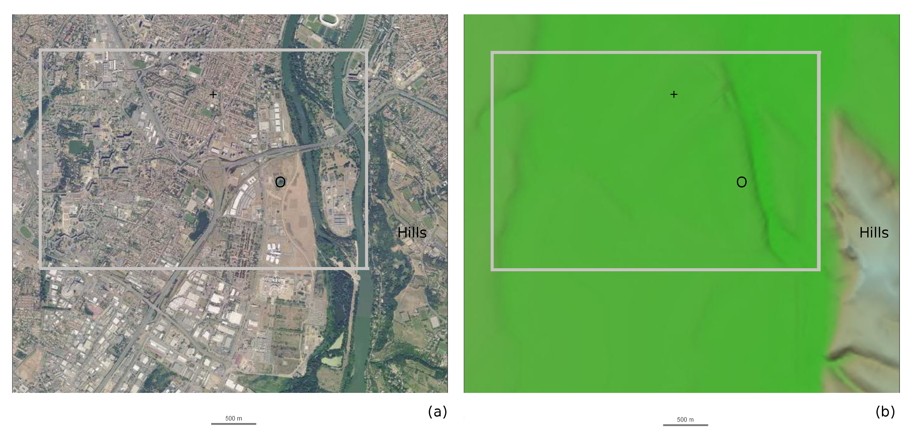
The local orography. Figure 1a provides an aerial view of the main districts affected by the fumes (bounded by a grey contour) and the factory (black circle). The elevation of the land at the boundary ranges from 140 m to 160 m. The ’Pech-David’ hills are located upstream of the factory, east of the Garonne River. The characteristic height of the hills is [90:120] m greater than that of the surrounding areas (Figure 1b). Apart from these hills upstream of the AZF plant, the non-constructed urban area is nearly flat.
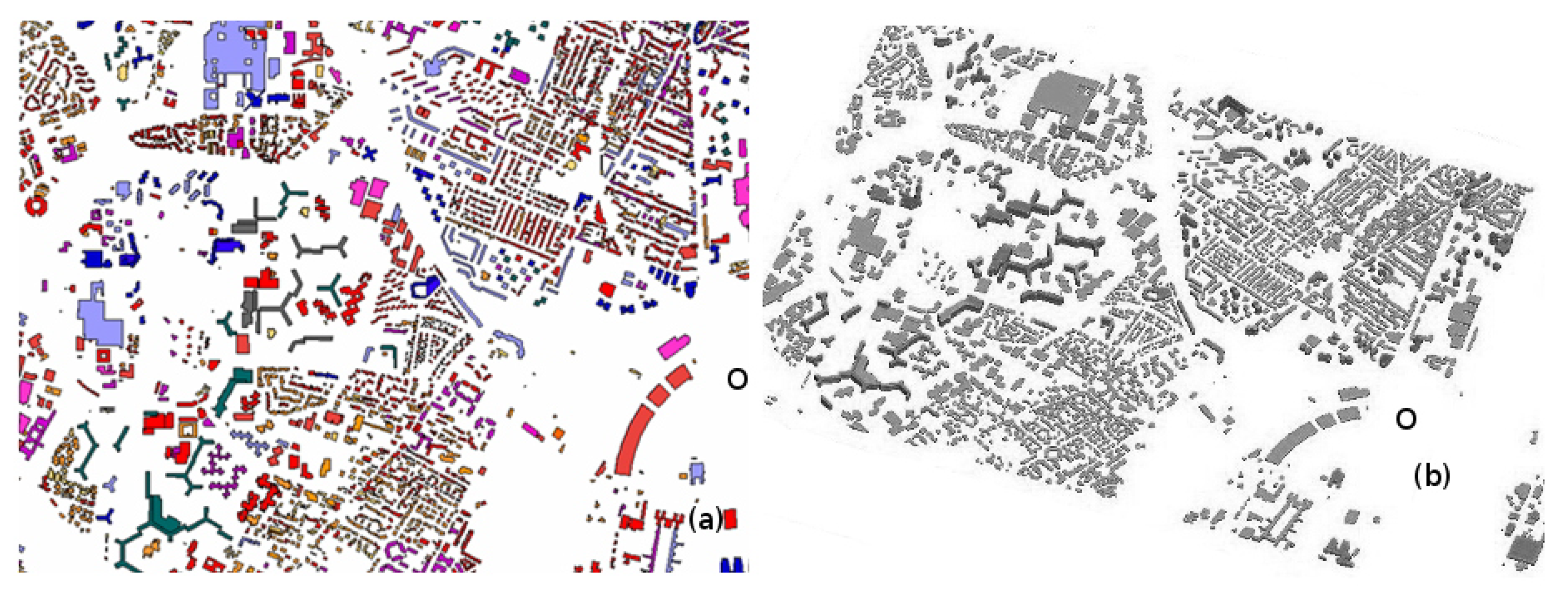
The city. The geometric information concerning the studied districts was provided by the IGN-BDTOPO database (IGN-BDTOPO: http://professionnels.ign.fr/bdtopo) and is illustrated in Figure 2a. This database provides the roof heights of the urban structures. The vectors normal to the roofs (resp. walls) are considered to be vertical (resp. horizontal). About 2700 buildings are documented in the database. Most of the buildings have a height of 5–10 m (Figure 2a), buildings of 10–20 m high are common, while the highest and sparsest buildings have heights between 30 m and 60 m.
The MNH-IBM grid. The modelling area covers km (Figure 1). We use a cartesian grid, isotropic for z lower than 100 m with a spatial grid resolution 2 m. Above 100 m, the mesh increases gradually in the vertical direction with a stretching of 1.05. The flow features (e.g., horseshow vortex, flow separations/reattachments) around buildings lower than 15 m could be considered vertically underresolved with this vertical resolution, but the objective here is to simulate the overall impact of the entire city and the friction effect, and not the specific flow in each canyon. The ceiling of the numerical domain is km. The effect of the upstream hills, in addition to the buildings, is modelled by IBM, as the terrain is flat in the coordinate system. Note that the IBM adaptation to terrain-following coordinate will constitute a future work. The discrete and complicated characteristics of the topographic database induce a specific methodology to build a continuous interface (see the Appendices). In the present study, the chosen computational grid dictates that the smaller houses with heights less than 5 m are not modelled and that the narrowest streets are merged with the surrounding buildings. Figure 2b illustrates the generated LSF related to the fluid–solid interface.
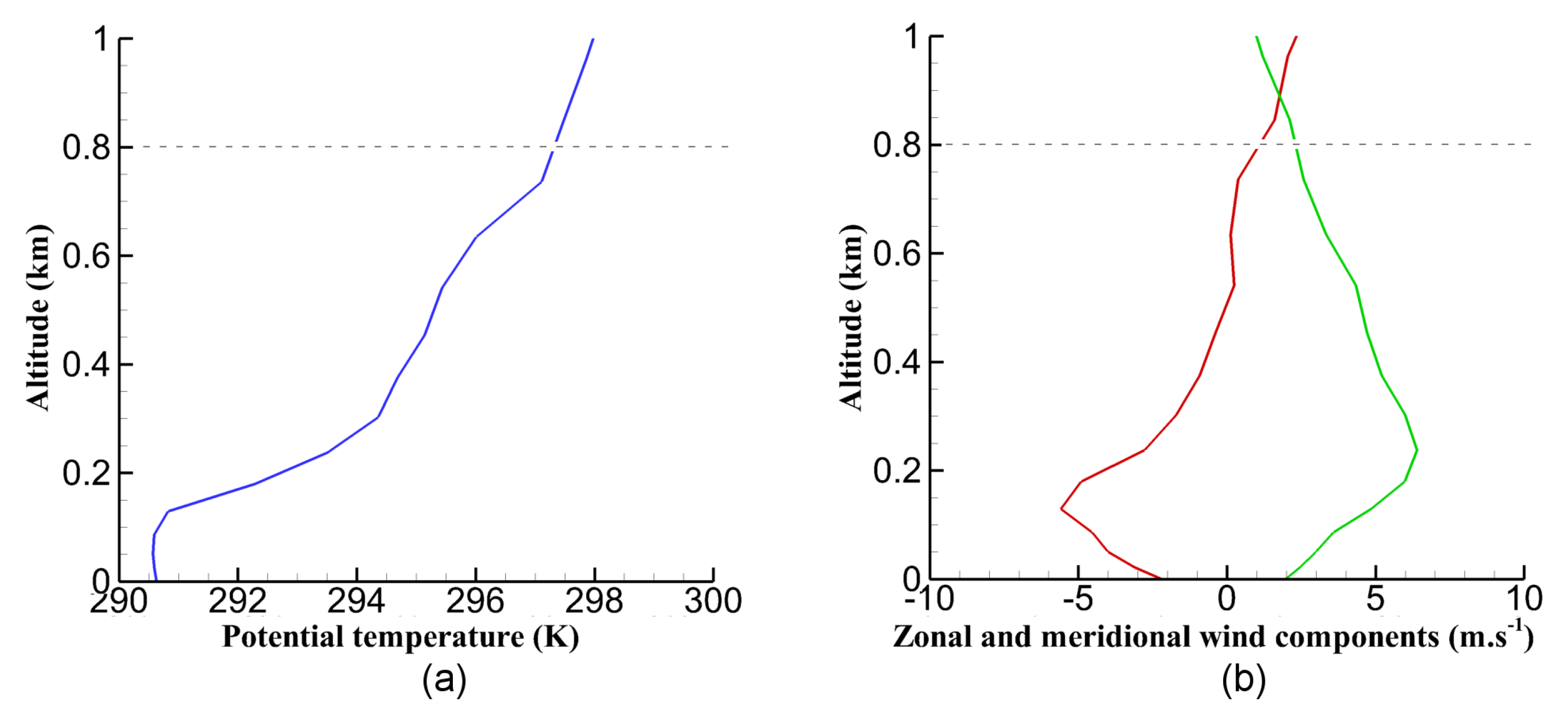
The atmospheric initial conditions. To generate the large-scale meteorological conditions on 21 September 2001 for the LES, a first mesoscale run is conducted with Meso-NH and without IBM over the 2 h 15 m prior to the explosion with interactive nested grids (three coarse resolutions: 2.5 km, 500 m, and 100 m), and is forced by the ECMWF operational analyses. Then, the LES is run in a single model with MNH-IBM over a short period (20 min), allowing to suppose steady large-scale fields, using the previous 100 m resolution fields of the nested run at 0815 UTC as initial fields. The morning conditions were sunny without cloud and with a water vapour mixing ratio of about 10 kg kg. The vertical initial profiles of the LES produced by the preliminary run at the AZF location are shown in Figure 3. The first layer above the ground presents a quasi-constant potential temperature and is capped by an inversion and the residual boundary layer, inducing a boundary layer (BL) height of approximately 200 m. The radiative heating at the ground, which forces non-zero values of the surface sensible heat flux, is still low at the time of detonation limiting the convective mixing. In this context, the MNH-IBM LES is assumed to be dry under near-neutral stability condition.
A south-east wind dominates near the ground (Figure 3b). Up to the top of the BL, the wind rapidly increases approaching a mean horizontal velocity of 8 m s. The wind direction turns towards the south at 400 m with a ∼ 4 m s speed. The zonal component in the free atmosphere dominates the meridional component (not shown here). This meteorological situation is frequently observed in Toulouse. The associated current at the lowest altitude is called the Autan wind and often induces moderate and severe wind speeds.
The incoming turbulence. While the atmospheric turbulence is not contained in the steady large-scale forcing, the near-neutral stability condition implies inlet turbulence in the BL governed by the surface friction. This is particularly true if large obstacles exist upstream of the studied zone. In the present case, the districts of Toulouse affected by the emissions are in the wake of a hilly region (the height of these hills is one order of magnitude higher than most of the buildings). The factory is located 10 from the hills. At the industrial plant location, the thickness of the turbulent layer is estimated to be 4–5 (the turbulent intensity strongly decreases above this height after the spin-up time). Therefore, it is realistic to assume that the turbulent layer downstream of the hills is predominantly governed by their presence. For these reasons and without IGN-BDTOPO information upstream of the study area, the hills (with a surface idealized by an elliptic shape approaching the real shape) and the buildings upstream (surface idealized by a cosine function with a ∼10 m wave number) are modelled by IBM to generate a realistic incoming turbulence. This is performed during an initial preliminary LES with IBM and without release to establish a turbulent state. During this run, the enstrophy, spatially integrated in the studied zone, increased up to a quasi-stationary value corresponding to a saturation state. This characteristic time of saturation was about 15 min. The four minutes following this saturation state provided four initial turbulent states that will be called the to initial conditions, in order to represent the chaotic nature of the atmospheric turbulence.
The numerical modelling. Far from the immersed interface (i.e., at grid points farther than one grid mesh from the interface in the fluid region), the wind advection scheme is either the fifth-order weight-essential-non-oscillatory (WENO) scheme associated with a third-order (five stages) explicit Runge–Kutta scheme (ERK) [24], or the fourth-order centred scheme associated with a fourth-order ERK and a numerical diffusion. Near the immersed interface (i.e., at grid points closer than one grid mesh from the interface), the wind transport scheme is either the third-order WENO scheme or the second-order centred scheme. Hence, the association of both schemes (far/near) presents an hybrid feature [11]. The subgrid turbulence kinetic energy (sTKE), potential temperature, and tracer are transported using a piecewise parabolic method (PPM) [25] associated with a forward–in–time algorithm. Large-scale fields (Figure 3) are imposed everywhere at the initialization. The top, bottom, and immersed interfaces are considered to be non-permeable. The homogeneous Neumann condition is applied at the top of the numerical domain on the tangential part of the velocity field (free-slip) and scalars. Open wave-radiation formulations [26] are employed at the lateral boundaries.
The friction coefficients for the ground between buildings are computed by SURFEX using a roughness length 0.1 m, as SURFEX deals with the unresolved urban obstacles, while the 3D shapes of buildings are explicitly resolved by the IBM. Additionally, a specific wall law based on a centimetric roughness length models the friction at the immersed interfaces. The surface sensible and latent heat fluxes are set to zero.
The Courant number never exceeds unity with a time step less than s. Most of the performed simulations cover the dispersion of the plume during the 15 min following the explosion. The simulations were executed on the OCCIGEN-CINES cluster on 2000 cores. The post-treatment (e.g., spatial integration) is performed in the area delimited by the grey contour in Figure 1.
The NO plume. Only limited information is available concerning the characteristics of the plume released after the explosion over the industrial site. Most people who observed its formation described the plume as an orange column with a 10 m diameter and a 10 m height. The order of magnitude of the diameter is consistent with the crater size. Cassadou et al. [20] mentioned similar plume scales in its initial stage. From these descriptions, the plume distribution is initialized as a vertical cylinder with a radius of 100 m radius and a height of 800 m (the vertical size of the numerical domain) at the AZF location. The cylinder numerically presents a homogeneous NO concentration in its core (the initial concentration in the plume is experimentally unknown). The pollutant is considered as a passive gazeous (no chemical transformation). Indeed, at the time of the explosion, the NO within the plume can be photodissociated on time scale of about 15 min. It will result in NO production that will eventually react with O to form back NO. Given the rather short duration of the simulations, the net NO production is rather limited and is neglected at this stage. We also assume zero background value. These assumptions and their impact are discussed in Section 6.
The measurement stations. The experimental data available to characterize the evolution of the pollutant plume are also limited. Only a few measurements from the ORAMIP are available and are discussed in Barthélémy et al. [21] and Cassadou et al. [20]. Four stations equipped with nitrogen dioxide passive samplers were within the plume path or in its vicinity. Three stations are located in Toulouse: ‘Maurice Jacquier’ school (43.5756 N, 1.41843 E) refered to here as ‘Jacquier’, ‘Pargaminières Street’, and ‘Metz Street’. The Jacquier Station is located 1.5 km north-west of the industrial site (the black cross in Figure 1). The two other urban stations are located in the town centre, 4 km north of the plant, and do not appear in Figure 1. The last station is located in Colomiers 10 km north-west of Toulouse. Between 0100 and 0400 UTC the day of the explosion, the four stations showed an usual nocturnal urban pollution with a NO concentration between 10 g·m and 60 g·m. After 0400 UTC, the NO concentration increased ([20:100] g·m) due to the urban traffic during this period.
At 0815 UTC, the Jacquier Station measured a normal NO concentration of [40:60] g·m, and the value climbed to 388 g·m at 0830 UTC. None of the other stations recorded so significant peak anomalies. In this paper, results are firstly discussed in terms of ratio to the initial concentration (Section 5). An estimation of the population exposure is then conducted assuming an initial concentration (Section 6).
5. Simulations of the AZF Case
As previously mentioned, the mesoscale nested domains have been run with time evolution and then the conditions at 0815 UTC have been used to run the LES with MNH-IBM in stationary conditions during 20 min, with four initial turbulent conditions, noted to . The instantaneous release of the accident at 0815 UTC is introduced in these LES to study the plume with different numerical schemes. The advection schemes are indeed a key component of LES as most of the eddies are resolved. Furthermore, in pollution studies, the implicit numerical diffusion impacts the spatial spread of the plume. Therefore LESs are conducted using either WENO () or centered () wind advection scheme where n is the space order. Different combinations of numerical schemes can be used between far and near the immersed interface. Three of them have been tested: W5/W3, C4/C2, and C4/W3 (far/near).
To physically simulate such an accident in a wind tunnel, a number of instantaneous releases (typically 100) would be performed and then averaged to provide reliable statistics. Here, no such ensemble averaging has been constructed, due to the computational cost: Depending on the numerical scheme, between 50,000 and 250,000 h are necessary for each LES. Therefore, a dozen of stationary LESs were performed, considering the different initial turbulent states and numerical schemes.
The characteristic height commonly used in air quality studies is 2 m, corresponding to a human size. In a city, this value gives information near the ground and does not represent the building scale ( 10 m is the characteristic height for the Toulouse case). To describe the surface layer near the ground, in the vicinity of the buildings, a vertical Gaussian integration is defined such that:
where , and P is a building presence function ( in a solid region and elsewhere). Additionally if . Equation (1) allows to weight f predominantly via and especially via , as levels near the ground constitue the area of interest. Table 1 presents the adopted symbol convention.
Section 5.1 discusses the sensitivity of these dynamical tests, and Section 5.2 focuses on the dispersive effects.
5.1. Sensitivity to Different Numerical Schemes
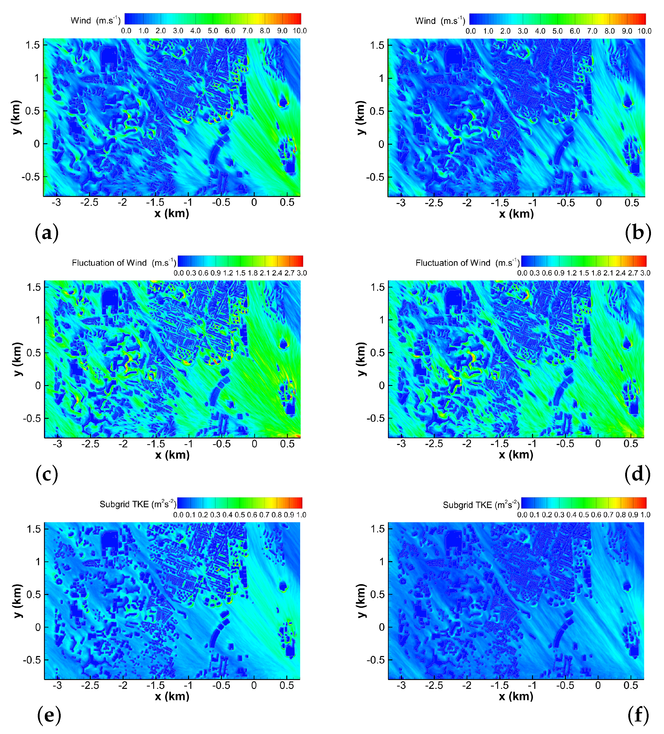
The 15-min averages of the Gaussian integration of the resolved wind, wind fluctuations, and subgrid turbulence kinetic energy (sTKE) are presented in Figure 4.
The left (resp. right) part shows the results of the C4/C2 (resp. W5/W3) advection scheme.
The time-averaged resolved wind (Figure 4a,b) shows values close to 5 m s in the areas with low building density, such as near the origin of detonation where the destroyed AZF buildings are not taken into account. The wind in the areas with high building density is often less than 2 m s. Some wind accelerations around buildings and in streets are sparsely detected and are associated with a maximum velocity of approximately 10 m s. The C4/C2 results are in good agreement with the W5/W3 ones. However, the deceleration of the wind due to the effective urban roughness is enhanced by the WENO scheme. Time-averaged wind fluctuations (Figure 4c,d) appear to be sensitive to the advection scheme in the regions of flow acceleration. The mean value of the wind fluctuations is about 1 m s. Some differences between the advection schemes are found in the sTKE results (Figure 4e,f). The production of sTKE with W5/W3 is much lower than that with C4/C2. Several regions of large sTKE values produced by C4/C2 disappear with W5/W3. This means that the implicit diffusion of the WENO scheme limits the explicit diffusion produced by the turbulence scheme.
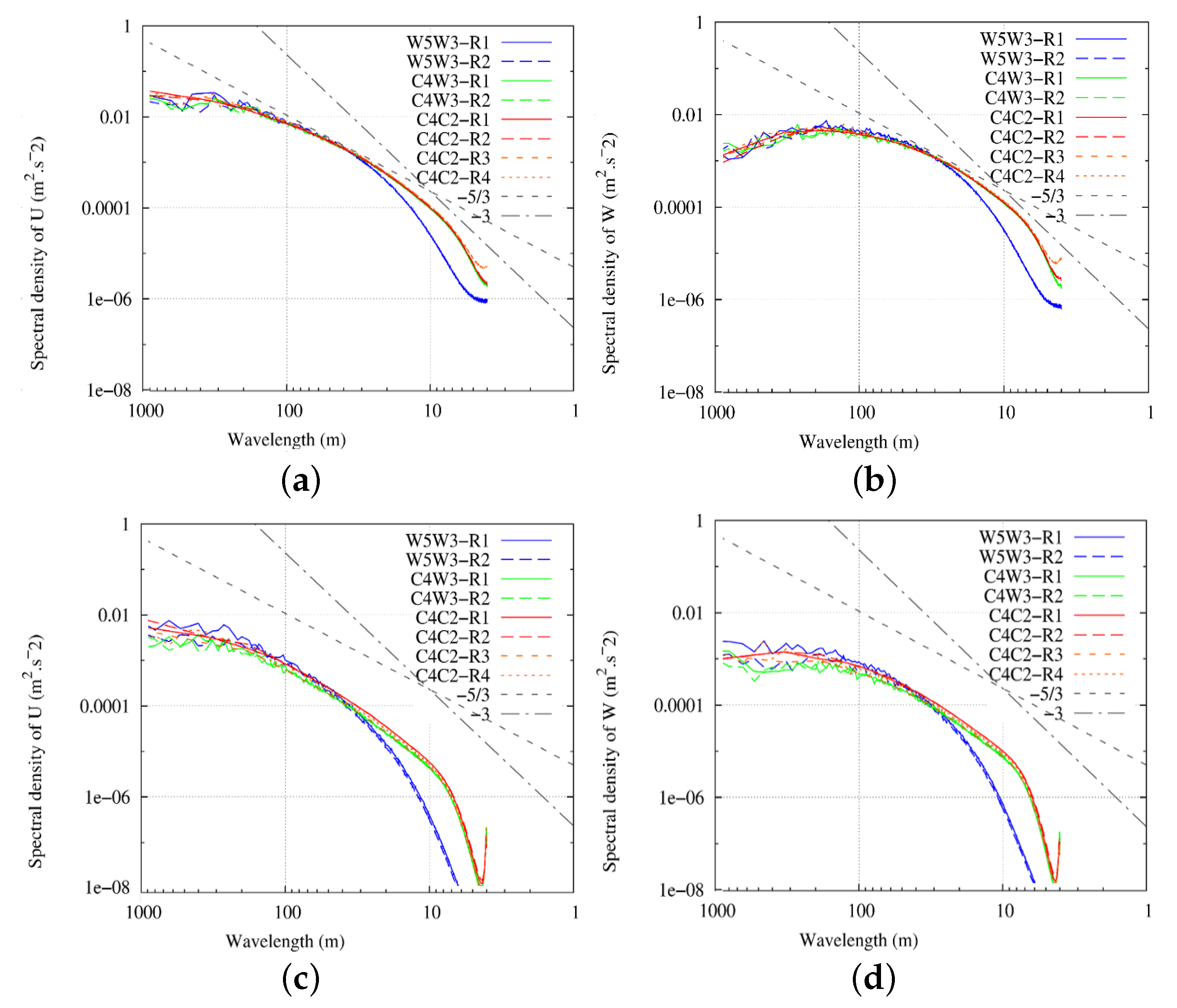
The Discrete Fourier Transform (DFT) is applied to zonal and vertical resolved wind components in the BL (Figure 5a,b) and above (Figure 5c,d) to get the energy spectra. The hybrid scheme combinations are plotted in each graph (colour code). A line type is associated with each run. The sensitivity study is therefore only based on a dozen of simulations. Except for the high wavelengths, the spectral density values are similar between the horizontal and vertical wind components, meaning a near-isotropic turbulent state. All the schemes match the slope well at wavelengths higher than the effective resolution (i.e., the scale from which the model departs from the slope, according to Skamarock [27]). But the sensitivity of numerical schemes acting far from the immersed interface exhibits significant differences in terms of effective resolution: C4 presents an effective resolution around , in agreement with previous studies [12,28], while it is coarser with W5, around (even coarser than Lunet et al. [24]), due to the implicit diffusion. Concerning the scheme used near the immersed interface, C4/C2 and C4/W3 are very similar, except in the BL (Figure 5-top) and near the cut-cell scale, where an energy increase can be found with C2. This increase is related to an energy accumulation generated at the immersed interfaces, due to a too low numerical diffusion. A higher numerical diffusion would be better appropriate to filter the numerical mode. Nevertheless, this increase remains weak and does not spread over the largest scales. In the same way, a similar energy increase is observed above the BL due to a too low artificial diffusion associated with C4. The amplitude of the high wave number modes above the BL is two orders of magnitude weaker than those in BL, showing more energy in the BL due to the resolved eddies generated by the canopy.
The energy spectra have shown a strong sensitivity of the wind transport schemes far from the fluid-solid interface in terms of effective resolution, with a coarser resolution with W5 than C4. But considering the scheme used in the vicinity of the obstacles, this sensitivity is strongly reduced. However the WENO schemes have been developed to better represent the solution in presence of high gradients, as in complex shock-obstacle interactions with IBM [29]. Therefore both WENO and CEN schemes will be considered in the following study.
5.2. Nitrogen Dioxide Dispersion
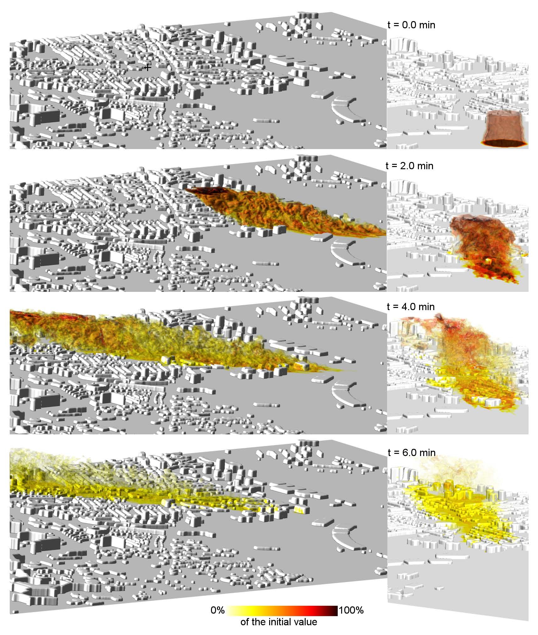
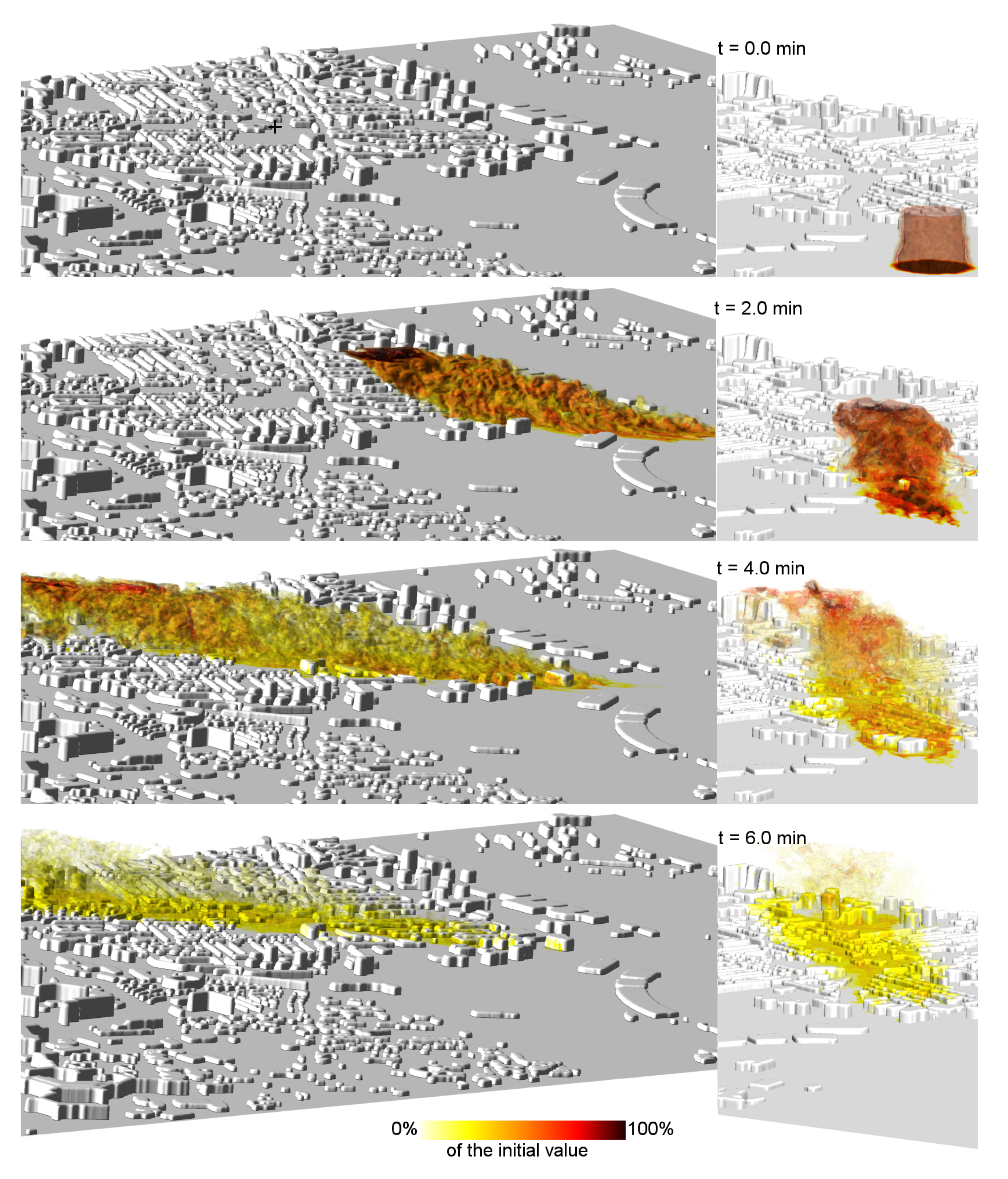
Figure 6-top illustrates the plume initialization ( 0 min) with two points of view. The dispersion of the plume over time is illustrated in the lower parts of Figure 6 at 2;4;6) min. The turbulent intensity near the ground is large (Figure 5) due to the nature of the incoming flow, the friction, the flow around the buildings and the vortex shedding in the building wake. As a consequence, the maximum value of the scalar concentration rapidly decreases and the plume spreads. Figure 6-bottom shows the persistence of around 10% of the initial concentration 6 min after the explosion (i.e., the emission). At this time, the areas affected by the plume are at least 2 (resp. 0.5) km in the direction parallel (resp. perpendicular) to the plume track.
In order to quantify the amount of pollutant reaching the Jacquier Station normalized by the initial concentration, Figure 7a shows the temporal evolution of the dimensionless concentration ratio, , computed at this location for different model integrations.
Three minutes after the beginning of the release, all simulations detect a plume occurrence at Jacquier. The [3:5] min period exhibits systematically a concentration peak. The range of the maximum simulated values at the Jacquier station is [0.1:0.5. The difference between these two concentrations highlights the plume dispersion and/or the distance of the station with the moving plume core.The simulated concentration falls below 10% of the initial concentration after 5 min and continues to decrease thereafter.
Figure 7b shows the diagram non dimensionalized by where is in the range [:] depending on the run. using W5 is lower than the maximum value obtained using C4 due to the diffusive behaviour of the WENO scheme. But the time-average value and the global tracer amount transported in the vicinity of the Jacquier Station are weakly dependent on the advection scheme type.
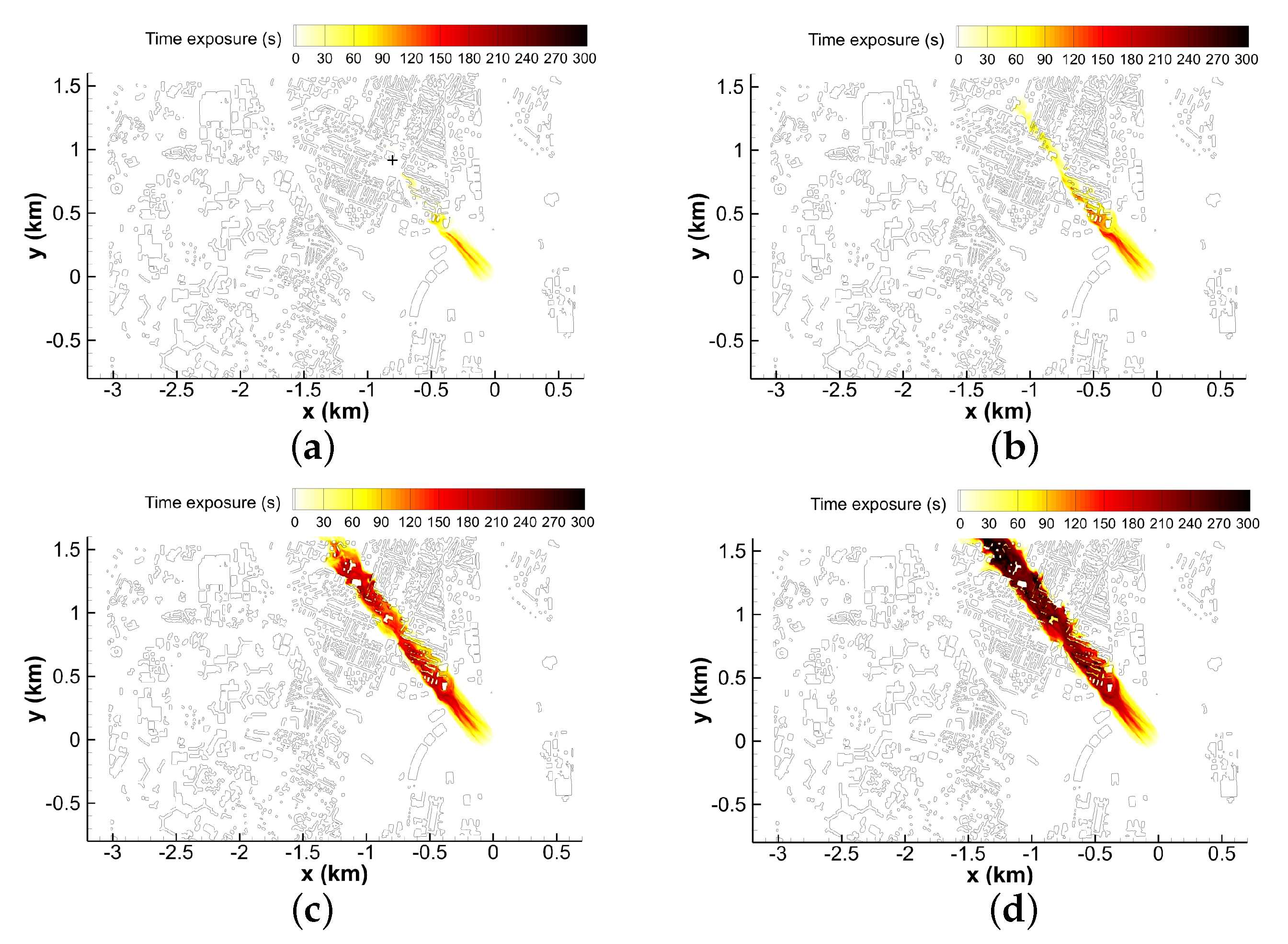
Two parameters affect the health impact due to the inhaled NO pollutant: The concentration value and the exposure time [20,23]. The local exposure time to a concentration higher than selected values is computed during the simulation. Four risk maps (for the C4/C2-R3 simulation) are illustrated in Figure 8 showing exposure times of 20%, 10%, 4%, and 2% of the initial concentration in panels (a, b, c, and d) respectively. The exposure time of higher than 20% never exceeds 1 min and is located in the vicinity of the AZF plant.
The exposure times for the highest values are slightly lower with W5 far from the immersed interface than those simulated with C4, and the width of the plume is larger by ∼10% for equal to 0.01 at a distance between the AZF plant and the Jacquier Station.
This study confirms that the wind advection scheme used far from the immersed interface with IBM impacts the spread of the plumes, in agreement with energy spectra. Conversely, the scheme used near the immersed boundary has almost no impact on the energy spectral distribution (the deviation between and is only observed at the small scales) and WENO schemes can be recommended to model the obstacle interactions.
6. Discussion on Population Exposure
The simulations allow to explore the population exposure in the AZF case. This firstly requires an estimation of the NO concentration at the initial state, considering different assumptions.
6.1. The Initial Plume Structure
As described previously, the NO concentration at the initial state of the simulation is assumed to be uniform in a 100 m wide cylinder with an altitude of 800 m. This simple assumption directly impacts the evolution of the pollutant distribution and requires some examination. Indeed, rare pictures of the plume shortly after the explosion (Internet sources) show a relatively homogeneous ochre colour due to the presence of NO. However, observers of the plume just after the explosion reported an increase in the colour intensity with altitude. This potential NO stratification could be related to a temperature increase near the ground at the time of detonation. The associated buoyancy effects could have induced a convective ascent transporting most of the NO to higher altitudes and contributing to variations in the opacity.
Nevertheless, retaining the assumption of an uniform distribution, three methods can be proposed to estimate the initial concentration as follows:
- Barthélémy et al. [21] mentioned an explosion of 1010 kg of ammonium nitrate. The maximum produced NO mass can be evaluated assuming that oxidation was complete and that all the nitrogen atoms formed the nitrogen dioxide. Assuming [4:8] dozen of tons of detonated ammonium nitrate [20], a plume with a volume of 5.10 m and an uniform NO distribution results in a mean concentration approaching [1:2] g m.
- Considering the ORAMIP measurement at the Jacquier Station, the passive sampler used for the measurement provides a NO value mean over 15 min which gives a dose estimate. Knowing the experimental value of 350 g m (the difference of the observed concentrations at Jacquier between 0830 and 0815 UTC), considering the plume dilution to be well–modelled by MNH-IBM and following the numerical results for (Figure 7b), the range of the presumed initial NO concentration is estimated to [10:30] mg m with a more likely value of 20 mg m 10 ppm (ratio defined by the mole fraction).
- Deedi [22] reported several concentration values from a study of the plume opacity. The few pictures of the initial plume lead to a 1010mg m NO concentration range.
The range of the NO estimate with complete oxidation is inconsistent with the other ones. While the assumption of an uniform vertical distribution is a substantial simplification, 20 mg m 10 ppm seems realistic near the ground and therefore this value will be considered in the following.
6.2. The Population Exposure
Considering this initial concentration, is estimated to be in the [2:10] mg·m range (Figure 7a). The risk maps (Figure 8) state that about 0.02 km were exposed to concentration of 4 mg·m during 1–2 min, and 0.2 km to 0.4 mg·m during 5–10 min. A near-linear dependence appears between the area covered by concentration and (not shown here).
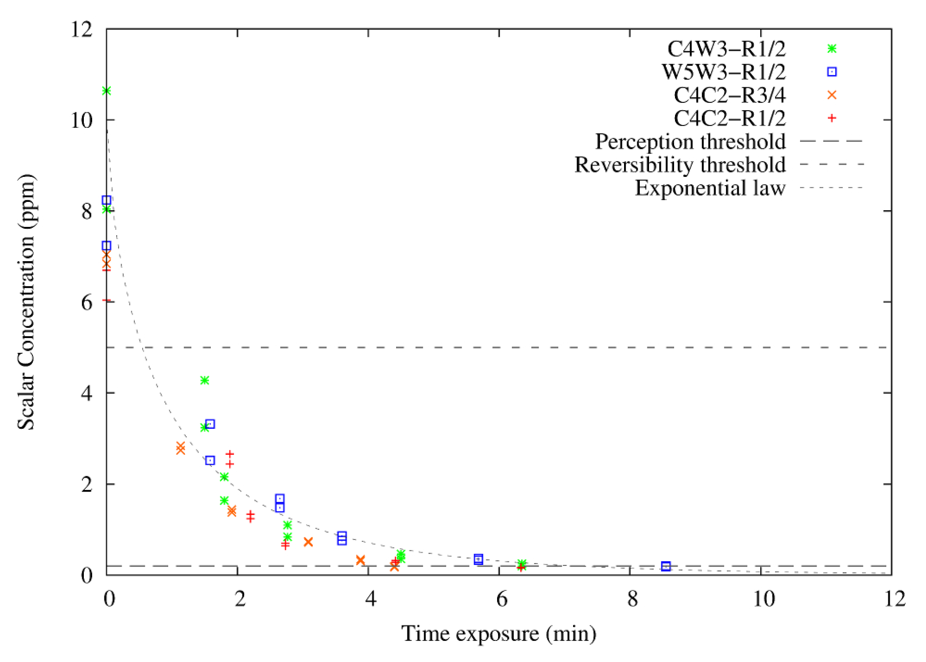
Considering the central axis of the plume, the evolution of the simulated pollutant concentration depending on the exposure time is shown in Figure 9. The perception (0.2 ppm) and reversibility (5 ppm) thresholds proposed by Tissot and Lafon [23] are also given, while the irreversibility threshold of 50 ppm is out of the range of simulated values. The perception threshold corresponds to the concentration leading to olfactory sensory detection. The reversibility one indicates when reversible effects (e.g., respiratory problems, nasal irritations, headaches, and asthenia) are encountered by the exposed population. In the immediate neighbourhood of the plant (a few hundreds of metres), population was exposed to reversible effects (Figure 8a). Beyond that distance, the exposition is a limited olfactory sensation (Figure 8d). In any case, no one should have experienced irreversible effects. These results are in agreement with the observations of doctors and firemen [21] and support the choice of near the ground.
To give an example of further investigation, the concentration level function of the exposure time can be fitted by the law , where the dimensionless time is , where = 5 m s is the characteristic horizontal plume velocity and 100 m is the horizontal scale of the plume (Figure 9). This formula gives an insight: When the velocity decreases, the diameter increases and the exposure time is longer.
7. Conclusions and Perspectives
This study reported numerical simulations of a pollutant episode in an urban environment linked to an explosion at a plant producing ammonium components. The selected case refered to the nitrogen dioxide emissions dispersed by the Autan wind after the dramatic explosion of the AZF factory that affected Toulouse in 2001.
The atmospheric flow has been simulated by the Meso-NH code coupled with SURFEX and including an immersed boundary method to account for buildings. A level-set function characterized the topography with an algorithm converting the BDTOPO-IGN database. Using the meteorological conditions that prevailed on the day of the explosion, a dozen of Large-Eddy Simulations were performed to conduct a preliminary sensitivity study on some dynamical parameters.
The results showed the ability of the numerical code to create a consistent energy spectrum in the surface boundary layer and in the lowest part of the atmospheric boundary layer. The impact of the wind advection scheme on the dynamic was also studied. The energy spectrum highlighted a more diffusive behaviour of the fifth-order WENO advection scheme at the micro scales and the relatively better behaviour of the fourth-order centred scheme coupled to an artificial hyper-viscosity term for which the diffusive amplitude has to be optimized. It pointed out that the wind advection scheme used far from the immersed interface impacted the spread of the plume, and may constitute a source of tuning in dispersion modelling, as well as a source of uncertainty for ensemble simulations. Conversely, the scheme used near the immersed boundary had almost no impact on the kinetic energy spectra and the WENO scheme can be recommended as it has been designed for obstacle interactions inducing sharp gradients.
Experimental measurements collected near the plant were used to estimate the released pollutant concentration under some assumptions. Assuming a passive pollutant, the numerical results allowed a risk map to be drawn showing the exposure time to concentrations of this potentially toxic gas. In reference to the thresholds concerning nitrogen dioxide adopted by French authorities (Quality threshold: 0.04 mg m; Information threshold: 0.2 mg m during 1 h; Alert threshold: 0.4 mg m during 3 h), the pollution episode due to the AZF case appeared to have been too brief to reach any of these thresholds, in good agreement with the conclusions of Cassadou et al. [20].
However, the first objective of this study was not to bring accurate answers to the AZF accident, but to show the potential of the immersed boundary method for urban applications. The method implemented in Meso-NH appears to be suitable to conduct preventative risk studies of pollution episodes within the near environment of industrial plants or airports, strongly affected by the impact of buildings.
In terms of perspective concerning the AZF case, the remaining uncertainties due to the crude description of the vertical distribution of the nitrogen dioxide concentration would need to be reduced to predict the absolute concentrations. The lack of experimental usable data is very challenging: The knowledge of the temperature increase due to the explosion would be a first input required to model the buoyancy effects, and to improve the source term. A numerical way could also be to directly model the explosion dynamics and the chemical reactions; however, this is a real scientific challenge (due to the multiple scales, compressibility hypothesis, reactive species, and code coupling). The nitrogen dioxide species is focused on here, but the risk maps can be applied to other potentially dangerous and reactive species.
To physically simulate an environmental accident, and to properly approach the chaotic character of the atmosphere, a number of instantaneous releases (typically 100) could be performed and then averaged to provide reliable statistics. However, the construction of an ensemble with LES is very expensive. Combining LES with a reduced-order model could be a solution to limit the computational cost and increase the set size.
Author Contributions
F.A. developed the IBM in Meso-NH, performed the simulations and post-processing, and redacted the main text; C.L. provided the preliminary run with Meso-NH without IBM and contributed to the redaction; V.M. and D.C. contributed to the analysis of the results. All authors have read and agreed to the published version of the manuscript.
Funding
This research received no external funding.
Acknowledgments
For stimulating discussions and contributions, the authors thank: R. Schoetter (Centre National de Recherches Météorologiques), J.-L. Redelsperger (Laboratoire de Physique des Océans, IFREMER, Brest), J.-P. Pinty and J. Escobar (Laboratoire d’Aérologie, Toulouse), O. Thouron and F. Blain (CERFACS). The simulations have been performed on the Nemo-CERFACS supercomputers and on the Occigen-CINES Bull cluster (GENCI projects: C2016017724 and A0010110079). This work has received support from the ’Région Midi-Pyrénées’. We dedicate this work to the memory of the AZF victims and hope to contribute to the thoughts and considerations of future green cities.
Conflicts of Interest
The authors declare no conflict of interest.
Abbreviations
The following abbreviations are used in this manuscript:
| AZF | Azote de France |
| BL | Boundary Layer |
| CCT | Cut-Cell Technique |
| DFT | Discrete Fourier Transform |
| ERK | Explicit Runge-Kutta scheme |
| GCT | Ghost-Cell Technique |
| IBM | Immersed Boundary Method |
| LES | Large Eddy Simulation |
| MNH-IBM | IBM adapted to the Meso-NH model |
| MUST | Mock Urban Setting Test |
| ORAMIP | Observatoire Régional de l’Air en Midi-Pyrénées |
| PPM | Piecewise Parabolic Method |
| SSF | Surface State Function |
| SSI | Surface State Index |
| WENO | Weight-Essential-Non-Oscillatory |
Appendix A. Surface State and LevelSet Function
Data characterizing a city include the coordinates of the building heights. Before generating the 3D LevelSet Function [19], noted , this field is discretized as the bottom limit of the numerical domain. A Surface State Function, , is defined where are the horizontal coordinates and n is the node type. Four node types per cell are available (on a 2D staggered grid): the mass, velocity and two geometric nodes. where no building is detected and gives the height of a detected solid structure. The nearest node of a database point is considered to be a roof point. is standardized per type of node such that, if a studied node is surrounded by four nodes of an other type, the studied node has characteristics of the surrounding points.
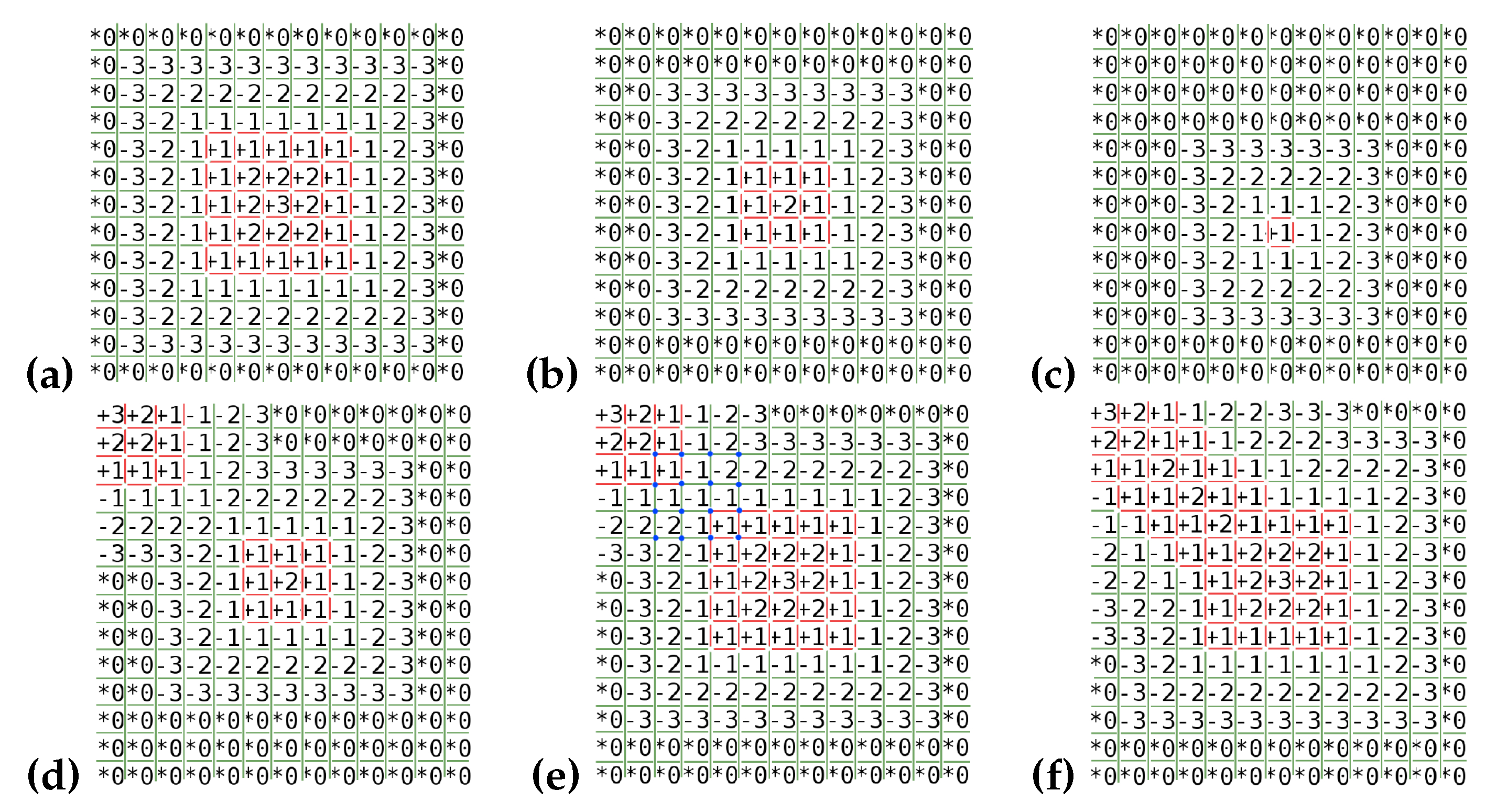
The next processes eliminate spacings that are too small and structures that IBM cannot resolve [11]. The problem is split into vertical and horizontal parts. The height, H, of each structure is compared to the vertical grid resolution, . If the structure is considered to be unresolved and is therefore filtered. If [2:4], H is increased up to 4 and the structure is considered to be vertically resolved. To treat the horizontal part, a Surface State Index, , characterizes the three cell layers around the fluid–solid interface. The first (resp. second and third) layer takes the value (resp. or ). The positive (resp. negative) -sign is related to the solid (resp. fluid) location ( outside of these layers). Figure A1a–c illustrate for three square obstacles. The red (resp. green) lines indicates the solid (resp. fluid) region at the ground elevation. The obstacle in Figure A1a is assumed to be spatially and horizontally resolved. Figure A1b,c illustrate two unresolved cases. Depending on , the process classification is summarized in Table A1. The spatial scales of the structure () and the spacing between the structures () are estimated as indicated by the ± symbol. (resp. ) corresponds to the Surface State Index of the studied node (resp. surrounding nodes).
- P1: If , no process is expected (Figure A1a).
- P3: If and , the ‘filtering’ process is activated. The obstacle shown in Figure A1c disappears.
- P4: The proximity of the obstacles (or spacings) can induce a ‘merging’ process testing = ±1 and (opposite sign). This is performed once in all grid directions and a second time only in the diagonal directions to limit the ‘stair-step shaped edges’ effect (Figure A1d–f). Figure A1d shows a small obstacle in the domain centre and another obstacle in the top-left corner. The ’increasing’ process (P2) is activated and the obstacle in the centre is extended. The first step of the ’merging’ process (P4) affects the median height of the two obstacles for cells detected at the blue points (Figure A1e). The second ’merging pass’ softens the border of the merged blue region (Figure A1f).
Note that the previous standardized procedure applied to is recalled during the processes (only one node type is shown here).

Table A1.
Modifications of the horizontal obstacle size depending on the Surface State Index ().
| Process | Class | Direction | Local | Surrounding |
|---|---|---|---|---|
| P1 | Nothing | All | . | |
| P2 | Increasing | All | ||
| P3 | Filtering | All | ||
| P4 | Merging | All |
Figure A1.
(a–c): Situations depending on the Surface State Index () inducing processes on the horizontal obstacle size: (a) Nothing (); (b) Increasing (); (c) Filtering (). (d–f): Process combinations on the horizontal obstacle size function of : (d) Reference state is two bodies; (e) Increasing one; (f) Merging the two bodies. The red contours indicate the presence of the obstacle. The green contours indicate the non-presence of the obstaclee. The blue points indicate the region to be merged.

The constructed is then used to generate the (seven points are defined in each cell, Appendix B). The first step of the -generation is the -initialization without obstacles only taking into account the ground (i.e., the vertical stratification of the function). The second step computes the distance to the vertical walls, which affects the minimal distance to the ground or the vertical walls. The third step computes the minimal distance to the roofs indicating the -sign: if the point presents a non-zero value of , ; otherwise, . The standardized procedure applied to the -sign eliminates some of the spurious interface effects. Finally, the smoothing technique is performed on the -function (Appendix B).
Appendix B. Smoothing Technique and LevelSet Function
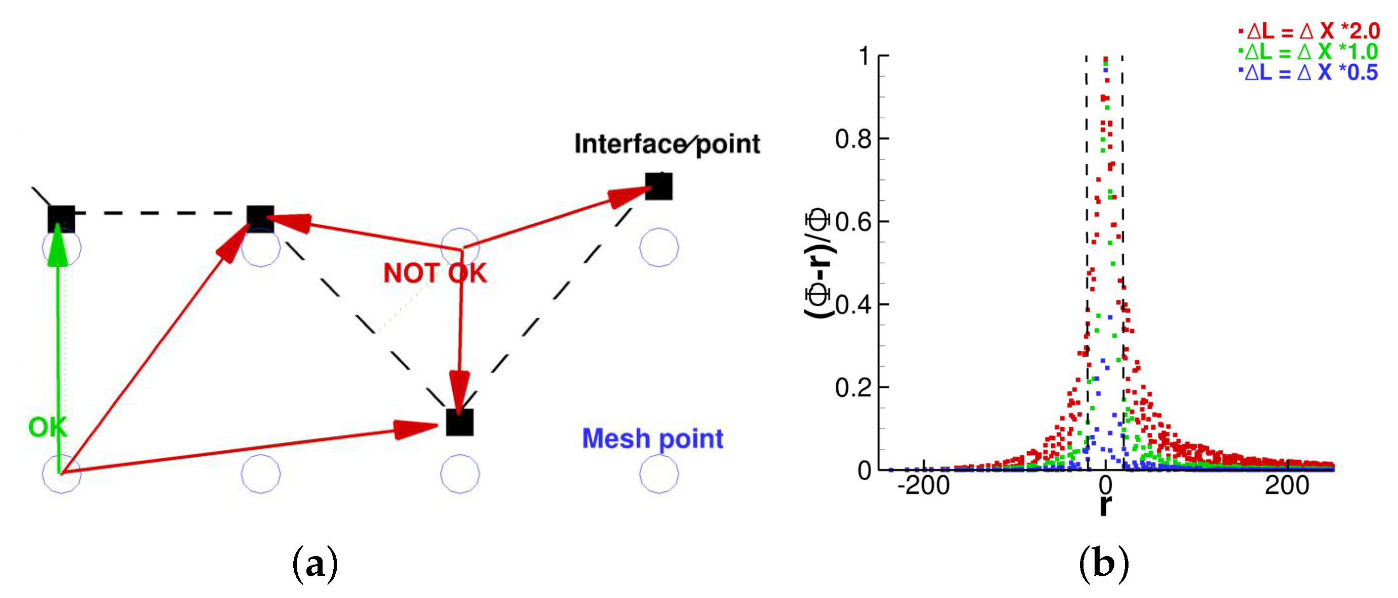
A fluid–solid interface characterized by a discrete signal introduces some numerical errors to the computation of the LevelSet Function (LSF, ). Figure A2a illustrates this via two cases. The mesh point in the left-bottom part of the figure has a correct -value due to the interface distance defined by the green arrow. Otherwise, the point in the right-top part of the figure computes a too large minimum -value with respect to the interface location (the black dashed line). The first method to limit such discretization errors is to estimate at several points per mesh cell: At the mass point denoted P, at the velocity points denoted and at the vorticity points denoted . The high number of points per cell improves the mathematical operations leading to a better approximation of the surface characteristics (i.e., the vector normal to the interface and the local curvature, ).
Figure A2.
(a) Errors introduced by the discrete nature of the interface during the LSF computation; (b) Dependence of the LSF-relative uncertainty () with the resolution ratio (cylinder case).
Figure A2.
(a) Errors introduced by the discrete nature of the interface during the LSF computation; (b) Dependence of the LSF-relative uncertainty () with the resolution ratio (cylinder case).

Moreover, a -artificial diffusion is implemented to preserve satisfaction, e.g., a redistanciation procedure. Note that this property is not intrinsically compatible with shape interfaces presenting singularities even if a redistanciation step is performed.
Defining a smooth weighting, Q, () is spread such that:
where are the neighbouring points. An iterative procedure applied for Equation (A1) is activated everywhere, with N the iteration number. Q and N are two unknown control parameters. A parametric study of the -generation depending on the resolutions ratio (Appendix C), for various objects showed a relative error that evolved as . This formulation is briefly illustrated in Figure A2b showing the -error exponentially decreasing with the interface distance (cylinder case). This behaviour motivates the Q-formulation, e.g., . The dimensionless constant is closely related to N. The first parameter acts as a smooth strength and the second one as a smooth propagation. Note that several attempts were made to introduce a convergence criterion based on the formulation ; however, the results were not found to be relevant.
The bell case (Appendix C) has been thoroughly investigated (via grid resolution and resolution ratio parametric studies) for two Agnesi shapes presenting large or small percent slopes. This investigation examines a sensitivity of the smoothing formulation to . Low values do not sufficiently correct the spurious effects. Too high values cause the solution to diverge. fits the expected interface well.
Appendix C. Geometric Properties and LevelSet Function
The accuracy of the interface recovery is primarly affected by the fineness of the resolution of the field data and that of the numerical domain (Appendix A). This section attempts to show the impact of these discretizations and that of the smoothing technique (Appendix B) on the modelling of ideal obstacles via the -function (LSF).
The fineness of the resolution, , of some discrete functions (the known field data) is studied here by varying the regular Cartesian grid (the resolution). Three bodies are approached: A disk or infinite cylinder (2D case, R is the radius), a cube (3D case, L is the side length), and an Agnesi hill (3D case, H is the height). The grid resolution is chosen to satisfactorily model the flow around the solid body [11]: , , and . In addition to the resolution study, the benefits of the -smoothing are discussed.
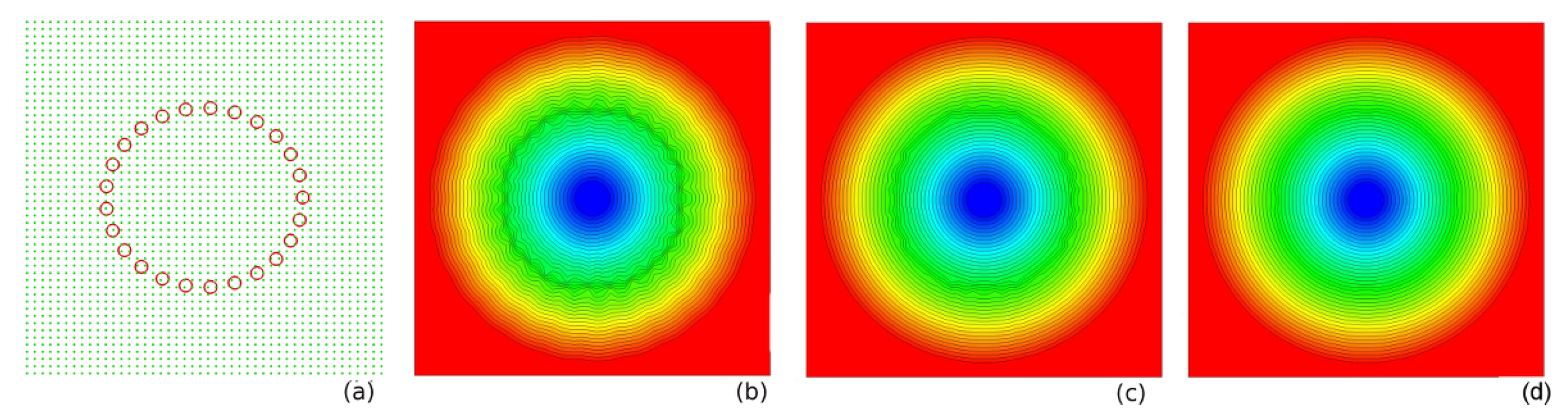
The cylinder case. The disk perimeter is discretized by points. The studied resolutions ratios are with an illustration of the -case in Figure A3a. is constructed using the procedures described in Appendix A. Most of the numerical errors are found in the vicinity of the interface. Figure A3b–d plot four dozens -values ( with respect to the scale of Figure A3a) and highlight the spurious effects at the interface. The maximum relative error on the location for (resp. ) is about (resp. ).
Figure A3.
(a) Illustration of the resolution ratio where is the mesh (resp. interface) space step in green symbols, where is the interface space step in red symbols. The -contours are shown without smoothing for = [(b) ; (c) ; (d) ] (cylinder case).
Figure A3.
(a) Illustration of the resolution ratio where is the mesh (resp. interface) space step in green symbols, where is the interface space step in red symbols. The -contours are shown without smoothing for = [(b) ; (c) ; (d) ] (cylinder case).

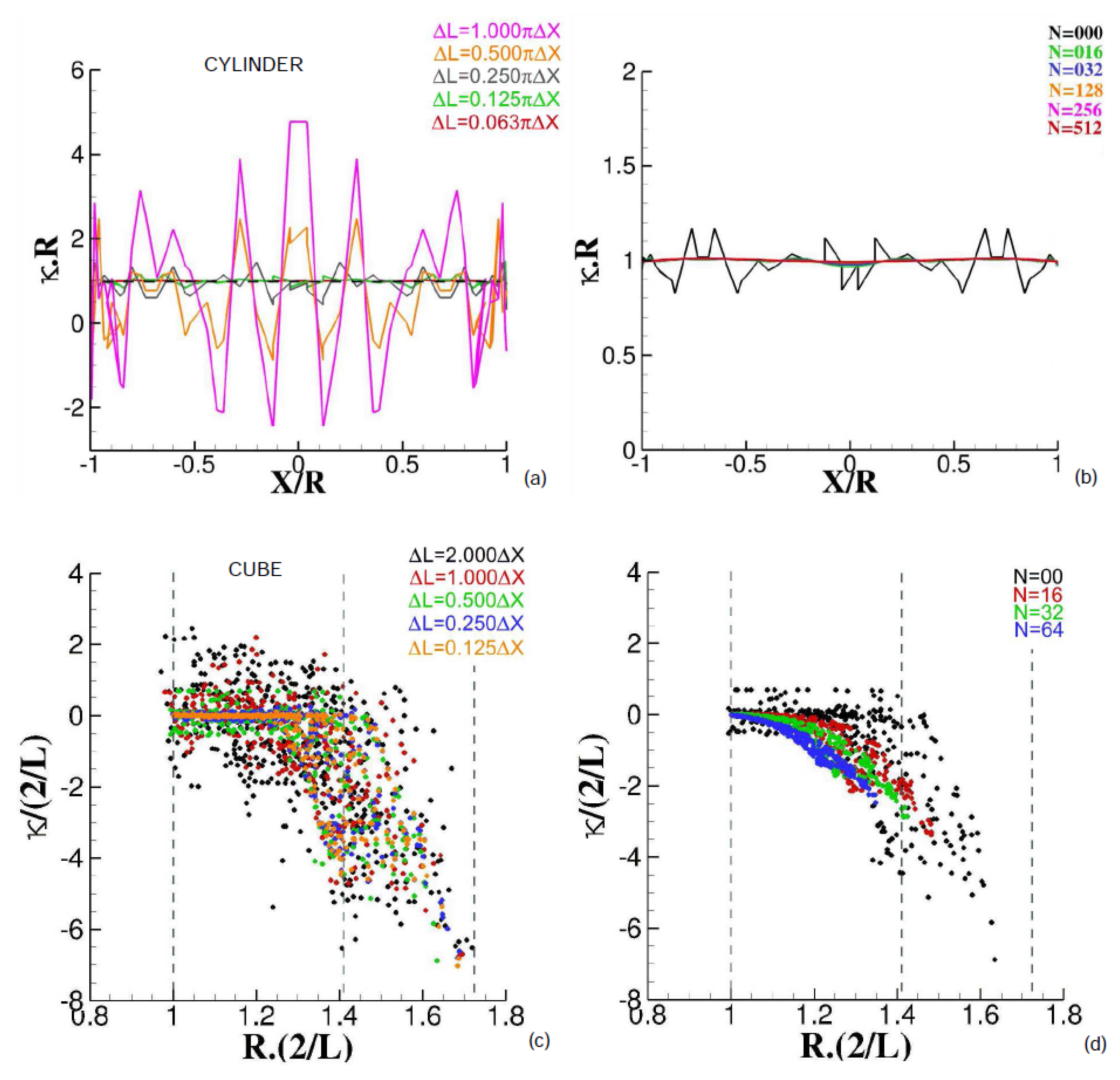
The numerical interface curvature, , is compared to the theoretical one () and plotted in Figure A4a for . The nature of the interface can be perceived numerically either as concave or convex, which can be problematic during a CFD simulation (a strong mistake compromises the incompressibility , where is the velocity field and is the fluid density). The -results become consistent for . Figure A4b shows the impact of the smoothing technique (Appendix B) on the local curvature fixing the resolution ratio to and varying the N iterations number of the smoothing technique. Without smoothing (), the -relative error is ∼20%. With , the relative error is decreased by a factor of . Note that the case of the sphere has been investigated and demonstrated similar results.
Figure A4.
Interface curvature for the cylinder (a,b) and cube (c,d) cases: (a) and (c) impact of the resolution ratio with ; (b) and (d) Impact of the N smoothing level with (b) and (d) . For the cylinder case, X is the projection of the interface location on an arbitrary axis of the R radius. For the cube case, R is the radial distance of the interface to the cube centre with a length L.

The cube case. The orientations of the cubic body (L is the side length) and the Cartesian grid influence the accuracy of the perceived geometric properties of the cube. A fully aligned cube with a resolution ratio yields the theoretical solution for (the factor comes from the use of a staggered grid). However, the numerical errors significantly increase when the parallelepipeds are not aligned with the grid. The most extreme case studied here corresponds to a cube whose faces present an angle of 45 degrees to those of the mesh (Figure A5a). The range of the resolutions ratio is . Figure A4c plots the curvature (nondimensionalized by ) depending on the resolutions ratio (colour code) and the location of the interface points (defined by the distance to the cube centre, written R, and nondimensionalized by ). corresponds to the centre of the cube surfaces and (resp. ) corresponds to the edges (resp. corners) of the cube. The local curvature at the cube interface is theoretically zero at all points except at singularities (edges and corners), where . Figure A4c demonstrates that the planar characteristic of the cube surfaces is clearly not respected for with smoothing (the black, red, and green points). Some computed curvature values are as large as those of a sphere with a radius of . The results become acceptable for (the blue and orange points in Figure A4c) even if the singularities have an influence for .
Figure A5.
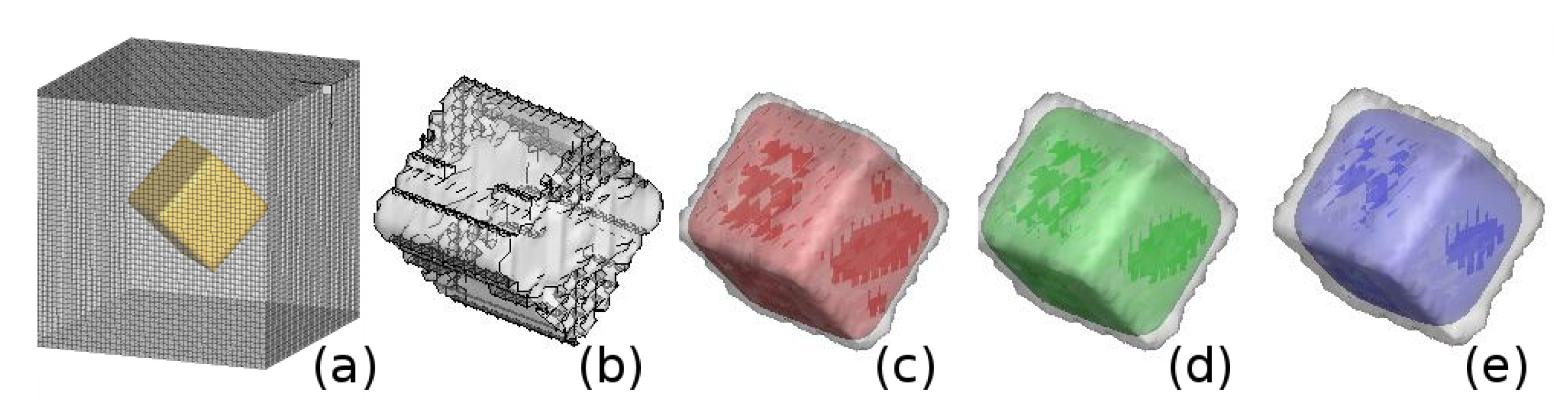
LSF generation: (a) Illustration of the discrete interface (in yellow) not correlated with the mesh. The -contour is visualized with for four N smoothing levels: (b) ; (c) ; (d) ; (e) (cube case).
Figure A5.
LSF generation: (a) Illustration of the discrete interface (in yellow) not correlated with the mesh. The -contour is visualized with for four N smoothing levels: (b) ; (c) ; (d) ; (e) (cube case).

The anisotropic nature of the cubic body is not compatible with the isotropic smoothing procedure. Indeed the corners and edges are rounded and the expected shape is not preserved. Both changes are illustrated in Figure A5b–e fixing the resolution ratio to for several N iteration number (from right to left: in blue, in green, in red and in grey). The disappearance of the rough surface depending on the N-smoothing is visible; however, a non-desired decrease of the cube volume appears with the smooth technique. The more N increases the more higher value decreases; the high -value vanishes by a factor for . In the same way, a finer grid resolution (L up to ) limits the spread and confines the smoothing action to the corner and ridge zones.
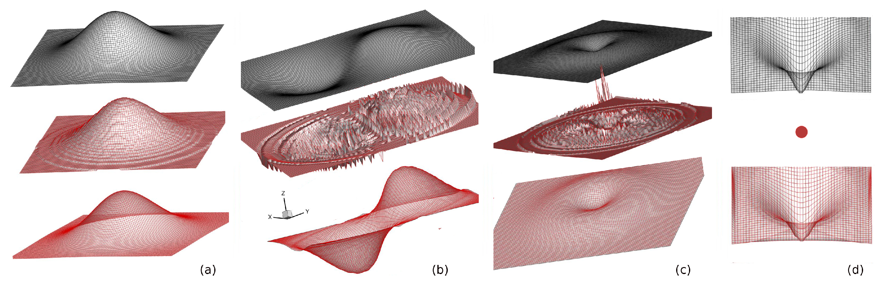
The bell case. Figure A6 shows the geometrical properties of an interface discretized by . From left to right are: (a) the altitude ; (b and c) the components of the vector normal to the interface , and (d) the local curvature . The black contours are the analytical solutions. The numerical solutions are plotted in red without (resp. with) the smooth technique in the middle (resp. bottom) panels of Figure A6. Without the smoothing technique, the maximum relative error are , and . With the smoothing technique , the results are , , and .
Figure A6.
Geometric properties: (a) altitude; (b) Horizontal component of the normal vector to the interface; (c) Vertical component of the normal vector to the interface; (d) Local curvature . indicates the horizontal interface location of the interface. z corresponds to the studied variable. The top panels show the analytical solution in black. In red, the numerical solutions are plotted without the smoothing technique in the middle of the panels. In red, the numerical solutions are plotted with the smoothing technique in the bottom of the panels. The poor numerical curvature without smoothing is not presented (bell case).

To summarize, the coupling of the interpolating and smoothing procedures appears to be the most viable method to properly estimate the complex and discrete surfaces. Associated with resolution ratio due to the staggered grid, iterations of the smoothing technique remain relevant and appear to be a good solution compared to the too expensive computation times (or the non-accessibility) of higher resolutions ratios.
References
- Santiago, J.; Dejoan, A.; Martilli, A.; Martin, F.; Pinelli, A. Comparison between large-eddy simulation and Reynolds-averaged Navier–Stokes computations for the MUST field experiment. Part I: Study of the flow for an incident wind directed perpendicularly to the front array of containers. Bound.-Layer Meteorol. 2010, 135, 109–132. [Google Scholar] [CrossRef]
- Milliez, M.; Carissimo, B. Numerical simulations of pollutant dispersion in an idealized urban area, for different meteorological conditions. Bound.-Layer Meteorol. 2007, 122, 321–342. [Google Scholar] [CrossRef]
- Onodera, N.; Aoki, T.; Shimokawabe, T.; Kobayashi, H. Large-scale LES wind simulation using lattice Boltzmann method for a 10 km × 10 km area in metropolitan Tokyo. TSUBAME E-Sci. J. Glob. Sci. Inf. Comput. Cent. 2013, 9, 2–8. [Google Scholar]
- Bergot, T.; Escobar, J.; Masson, V. Effect of small scale surface heterogeneities and buildings on radiation fog: Large-Eddy Simulation study at Paris-Charles de Gaulle airport. Q. J. R. Meteorol. Soc. 2015, 141, 285–298. [Google Scholar] [CrossRef]
- Mittal, R.; Iaccarino, G. Immersed boundary methods. Annu. Rev. Fluid Mech. 2005, 37, 239–261. [Google Scholar] [CrossRef] [Green Version]
- Aumond, P.; Masson, V.; Lac, C.; Gauvreau, B.; Dupont, S.; Bérengier, M. Including the drag effects of canopies: Real case large-eddy simulation studies. Bound.-Layer Meteorol. 2013, 146, 65–80. [Google Scholar] [CrossRef]
- Tseng, Y.H.; Ferziger, J.H. A ghost-cell immersed boundary method for flow in complex geometry. J. Comput. Phys. 2003, 192, 593–623. [Google Scholar] [CrossRef]
- Lundquist, K.A.; Chow, F.K.; Lundquist, J.K. An immersed boundary method for the weather research and forecasting model. Mon. Weather Rev. 2010, 138, 796–817. [Google Scholar] [CrossRef]
- Lundquist, K.A.; Chow, F.K.; Lundquist, J.K. An immersed boundary method enabling large-eddy simulations of flow over complex terrain in the WRF Model. Mon. Weather Rev. 2012, 140, 3936–3955. [Google Scholar] [CrossRef]
- Arthur, R.S.; Lundquist, K.A.; Mirocha, J.D.; Chow, F.K. Topographic effects on radiation in the WRF Model with the immersed boundary method: Implementation, validation, and application to complex terrain. Mon. Weather Rev. 2018, 146, 3277–3292. [Google Scholar] [CrossRef]
- Auguste, F.; Réa, G.; Paoli, R.; Lac, C.; Masson, V.; Cariolle, D. Implementation of an immersed boundary method in the Meso-NH V5.2 model: Applications to an idealized urban environment. Geosci. Model Dev. 2019, 12, 2607–2633. [Google Scholar] [CrossRef] [Green Version]
- Lac, C.; Chaboureau, J.P.; Masson, V.; Pinty, J.P.; Tulet, P.; Escobar, J.; Leriche, M.; Barthe, C.; Aouizerats, B.; Augros, C.; et al. Overview of the Meso-NH model version 5.4 and its applications. Geosci. Model Dev. 2018, 11, 1929–1969. [Google Scholar] [CrossRef] [Green Version]
- Lafore, J.P.; Stein, J.; Asencio, N.; Bougeault, P.; Ducrocq, V.; Duron, J.; Fischer, C.; Héreil, P.; Mascart, P.; Masson, V.; et al. The Meso-NH Atmospheric Simulation System. Part I: Adiabatic formulation and control simulations. Scientific objectives and experimental design. Ann. Geophys. 1998, 16, 90–109. [Google Scholar] [CrossRef]
- Masson, V.; Lion, Y.; Peter, A.; Pigeon, G.; Buyck, J.; Brun, E. Grand Paris: Regional landscape change to adapt city to climate warming. Clim. Chang. 2013, 117, 769–782. [Google Scholar] [CrossRef] [Green Version]
- Yang, G.; Causon, D.; Ingram, D.; Saunders, R.; Battent, P. A Cartesian cut cell method for compressible flows. Part A: Static body problems. Aeronaut. J. 1997, 101, 47–56. [Google Scholar]
- Piomelli, U.; Balaras, E. Wall-layer models for large-eddy simulations. Annu. Rev. Fluid Mech. 2002, 34, 349–374. [Google Scholar] [CrossRef] [Green Version]
- Bernardet, P. The pressure term in the anelastic model: A symmetric elliptic solver for an Arakawa C grid in generalized coordinates. Mon. Weather Rev. 1995, 123, 2474–2490. [Google Scholar] [CrossRef] [Green Version]
- Cuxart, J.; Bougeault, P.; Redelsperger, J.L. A turbulence scheme allowing for mesoscale and large-eddy simulations. Q. J. R. Meteorol. Soc. 2000, 126, 1–30. [Google Scholar] [CrossRef]
- Sussman, M.; Smereka, P.; Osher, S. A level set approach for computing solutions to incompressible two-phase flow. J. Comput. Phys. 1994, 114, 146–159. [Google Scholar] [CrossRef]
- Cassadou, S.; Ricoux, C.; Gourier-Fréry, C.; Schwoebel, V.; Guinard, A. Conséquences Sanitaires de l’explosion Survenue à l’usine AZF de Toulouse le 21 Sept. 2001 (Expositions Environnementales); Technical Report, Rapport du DRASS Midi-Pyrénées; Institute de Veille Sanitaire: Saint-Maurice, France, 2003.
- Barthélémy, F.; Hornus, H.; Roussot, J.; Hufschmitt, J.P.; Raffoux, J.F. Usine de la Société Grande Paroisse Toulouse—Accident du 21 Septembre 2001; Technical Report, Rapport de l’Inspection Générale de l’Environnement; Ministère de l’Aménagement du Territoire et de l’Environnement: Paris, France, 2001.
- Deedi. Management of Oxides of Nitrogen in Open Cut Blasting; Technical Report, Queensland Guidance Note, QGN 20, v3; Department of Employment, Economic Development, and Innovation: Barcaldine, Australia, 1999.
- Tissot, S.; Lafon, D. Seuils de toxicité aiguë utilisés lors d’émissions atmosphériques accidentelles de produits chimiques. Archives des Maladies Professionnelles et de l’Environnement 2006, 67, 870–876. [Google Scholar] [CrossRef]
- Lunet, T.; Lac, C.; Auguste, F.; Visentin, F.; Masson, V.; Escobar, J. Combination of WENO and Explicit Runge-Kutta methods for wind transport in Meso-NH model. Mon. Weather Rev. 2017, 145, 3817–3838. [Google Scholar] [CrossRef]
- Colella, P.; Woodward, P.R. The piecewise parabolic method (PPM) for gas-dynamical simulations. J. Comput. Phys. 1984, 54, 174–201. [Google Scholar] [CrossRef] [Green Version]
- Carpenter, K.M. Note on the paper ‘Radiation conditions for lateral boundaries of limited area numerical models’. Q. J. R. Meteorol. Soc. 1982, 110, 717–719. [Google Scholar] [CrossRef]
- Skamarock, W.C. Evaluating mesoscale NWP models using kinetic energy spectra. Mon. Weather Rev. 2004, 132, 3019–3032. [Google Scholar] [CrossRef]
- Ricard, D.; Lac, C.; Riette, S.; Legrand, R.; Mary, A. Kinetic energy spectra characteristics of two convection-permitting limited-area models AROME and Meso-NH. Q. J. R. Meteorol. Soc. 2013, 139, 1327–1341. [Google Scholar] [CrossRef]
- Chaudhuri, A.; Hadjadj, A.; Chinnayya, A. On the use of immersed boundary methods for shock and obstacle interactions. J. Comput. Phys. 2011, 230, 1731–1748. [Google Scholar] [CrossRef]
Figure 1.
(a) Aerial photograph of Toulouse and its hilly region (www.geoportail.gouv.fr); (b) Topographic map of the same zone. The MNH-IBM study area is bounded by a grey contour. The black circle indicates the location of the factory and the black cross indicates the Jacquier station. The green color indicates a near-flat terrain with a 150 m altitude above sea level.

Figure 2.
(a) IGN-BDTOPO database related to the bounded area in Figure 1: Yellow–orange–red colours represent buildings of 5–10 m height, purple–blue 10–20 m, and green-grey 30–60 m. (b) Recovery of the fluid–solid interface in the MNH-IBM domain modelled by the zero value of the LevelSet function. The black circle indicates the location of the factory in the two pictures. Figure 1’s legend informs about the space scale.

Figure 3.
Large-scale vertical profiles at 0815 UTC at the Azote de France (AZF) fertilizer plant location: (a) Potential temperature; (b) zonal (in red line), and meridional (in green line) components of the mean wind. The dashed lines indicate the height of the large-eddy simulations (LES) domain.

Figure 4.
Surface map of the 15-min averages of the Gaussian integration of variables 1 m above the ground: (a,b) Wind speed; (c,d) wind fluctuations; (e,f) subgrid turbulence kinetic energy. The left column shows the results of the advection scheme, and the right column .
Figure 4.
Surface map of the 15-min averages of the Gaussian integration of variables 1 m above the ground: (a,b) Wind speed; (c,d) wind fluctuations; (e,f) subgrid turbulence kinetic energy. The left column shows the results of the advection scheme, and the right column .

Figure 5.
Spectral density (a,b) in the boundary layer up to 200 m; (c,d) in the highest levels 200 m 800 m. (a) and (c) present the discrete Fourier transform (DFT) of the zonal wind component, (b) and (d) the DFT of the vertical wind component. The colour code indicates the advection scheme and the line type of the run depending on the spin-up.

Figure 6.
Four visualisations of the plume dispersion for the C4/C2-R3 simulation from the initial stage (top) until 6 min after the emission (bottom) with two view angles (left and right). The colour code indicates the ratio of pollutant concentration to the initial value (in %) with dark brown/black corresponding to the initial concentration. The ground and the buildings appear in grey. At min, the plume presents a length of 2 km and a width of 500 m.

Figure 7.
At the ’Maurice Jacquier’ primary school: (a) Temporal evolution of the scalar concentration (according to the initial value); (b) relationship between the mean and the maximum concentrations numerically observed within 15 min after the emission.
Figure 7.
At the ’Maurice Jacquier’ primary school: (a) Temporal evolution of the scalar concentration (according to the initial value); (b) relationship between the mean and the maximum concentrations numerically observed within 15 min after the emission.

Figure 8.
Exposure time (s) near the ground as a percentage of the initial pollutant concentration: (a) 20%; (b) 10%; (c) 4%, and (d) 2% from the C4/C2-R3 simulation. The black cross indicates the location of the Jacquier Station.
Figure 8.
Exposure time (s) near the ground as a percentage of the initial pollutant concentration: (a) 20%; (b) 10%; (c) 4%, and (d) 2% from the C4/C2-R3 simulation. The black cross indicates the location of the Jacquier Station.

Figure 9.
Estimate of the population exposure as a function of the NO concentration and the exposure time. The colour code and symbol style indicate the simulation type. Two thresholds are given by Tissot and Lafon [23].
Figure 9.
Estimate of the population exposure as a function of the NO concentration and the exposure time. The colour code and symbol style indicate the simulation type. Two thresholds are given by Tissot and Lafon [23].

Table 1.
Symbol and operation conventions for an arbitrary variable f.
| Notation | Definition |
|---|---|
| f | Local and instantaneous variable |
| Gaussian distribution near the ground | |
| 15 min integration |
© 2020 by the authors. Licensee MDPI, Basel, Switzerland. This article is an open access article distributed under the terms and conditions of the Creative Commons Attribution (CC BY) license (http://creativecommons.org/licenses/by/4.0/).
Share and Cite
MDPI and ACS Style
Auguste, F.; Lac, C.; Masson, V.; Cariolle, D. Large-Eddy Simulations with an Immersed Boundary Method: Pollutant Dispersion over Urban Terrain. Atmosphere 2020, 11, 113. https://doi.org/10.3390/atmos11010113
AMA Style
Auguste F, Lac C, Masson V, Cariolle D. Large-Eddy Simulations with an Immersed Boundary Method: Pollutant Dispersion over Urban Terrain. Atmosphere. 2020; 11(1):113. https://doi.org/10.3390/atmos11010113
Chicago/Turabian StyleAuguste, Franck, Christine Lac, Valery Masson, and Daniel Cariolle. 2020. "Large-Eddy Simulations with an Immersed Boundary Method: Pollutant Dispersion over Urban Terrain" Atmosphere 11, no. 1: 113. https://doi.org/10.3390/atmos11010113
Note that from the first issue of 2016, this journal uses article numbers instead of page numbers. See further details here.