Analysis of Raindrop Shapes and Scattering Calculations: The Outer Rain Bands of Tropical Depression Nate

Abstract

Tropical storm Nate, which was a powerful hurricane prior to landfall along the US Gulf coast, traversed north and weakened considerably to a tropical depression as it moved near an instrumented site in Hunstville, AL. The outer rain bands lasted 18 h (03:00 to 21:00 UTC on 08 October 2017) and a 2D-video disdrometer (2DVD) captured the event which was shallow at times and indicative of pure warm rain processes. The 2DVD measurements are used for 3D reconstruction of drop shapes (including the rotationally asymmetric drops) and the drop-by-drop scattering matrix has been computed using Computer Simulation Technology integral equation solver for drop sizes >2.5 mm. From the scattering matrix elements, the polarimetric radar observables are simulated by integrating over 1 min consecutive segments of the event. These simulated values are compared with dual-polarized C-band radar data located at 15 km range from the 2DVD site to evaluate the contribution of the asymmetric drop shapes, specifically to differential reflectivity. The drop fall velocities and drop horizontal velocities in terms of magnitude and direction, all being derived from each drop image from two orthogonal cameras of the 2DVD, are also considered.

1. Introduction

One of the important applications of polarimetric radar is the measurement of rainfall whose accuracy depends critically on the assumed drop shape model [1]. Beard and Chuang [2] numerically derived the shapes of drops under equilibrium conditions of balance between aerodynamic, surface tension and gravitational forces. However, rain drops (with D > 0.7 mm or so) oscillate due to wake instabilities or time-varying drag, but the oscillation modes (axisymmetric or asymmetric) and the distribution of oscillation amplitudes are not theoretically predictable. In laminar flow, the wind-tunnel experiments of Szakáll et al. [3] showed that larger drops (>2.0 mm) oscillate primarily in the axisymmetric oblate-prolate mode with smaller amplitude asymmetric modes mixed in. These wind-tunnel data (based on high speed camera images of different sized suspended drops for a few seconds) were consistent with the earlier 80 m fall ‘artificial rain’ experiment of drop shapes imaged as individual ‘snap shots’ with a 2D-video disdrometer (2DVD) [4,5,6]. This consistency was used to develop a mean axis ratio versus equi-volume drop diameter (D_eq) model by Thurai et al. [4] which is based on direct measurements of drop shapes after 80-m fall. The fundamental oscillation modes and shapes have been summarized in [7]. The dominant mode detected in the wind-tunnel data was the axisymmetric mode with smaller amplitude transverse modes also present. The latter mode has shapes which do not possess an axis of rotational symmetry (henceforth termed as asymmetric shapes) as a result of non-axisymmetric drop oscillations.

A relatively recent advance has been the use of 2DVD in reconstructing the 3D shapes of natural rain drops even if they are asymmetric [8,9] and further to calculate the scattering matrices of such asymmetric drops using advanced electromagnetic scattering codes [10,11]. This enables simulation of what is termed ‘drop-by-drop’ integration to arrive at the radar reflectivity, the differential reflectivity and the copolar correlation coefficient [12]. Comparing the ‘drop-by-drop’ with the ‘bulk’ simulations of the same event using the average oblate axis ratio versus D_eq relations enabled a determination of the importance of asymmetric shapes and their frequency of occurrence relative to the axisymmetric shapes, as in one example of an intense line convection [12,13]. However, in less intense convection or in pure warm rain process (coalescence) dominated events, the frequency of occurrence of asymmetric drops shapes and their impact on Z_dr is not known, which is the subject matter addressed herein. It is well known that small drops dominate the size distributions in tropical rain with active warm rain processes relative to ice dominated deeper convection [14]. It has been speculated that in the ice dominated cases, asymmetric shapes due to oscillations can be dampened by residual tiny ice cores in the nearly fully melted drops (originating as graupel or tiny hail aloft) [15,16]. On the other hand, pure warm rain processes have no such damping mechanism and thus might exhibit more frequent occurrence of asymmetric shapes.

The paper is organized as follows. In Section 2, we give an overview of tropical depression (TD) Nate and an outline of the specific instruments and measurements pertaining to this study. In Section 3, processing of the 2DVD-based images is presented, together with drop horizontal velocities which are obtained as a by-product of the deskewing procedure of the drop images. Section 4 outlines the scattering calculation procedure and Section 5 presents the single particle radar cross-sections calculated for all drops with D_eq > 2.5 mm as well as their differential reflectivities. In Section 6, the computed reflectivity and differential reflectivity based on the scattering calculations over a 1-min interval are compared with the C-band radar measurements over the instrument site, for the entire duration of the TD Nate event. The main conclusions are summarized in Section 7.

2. TD Nate Description and Observations in Huntsville

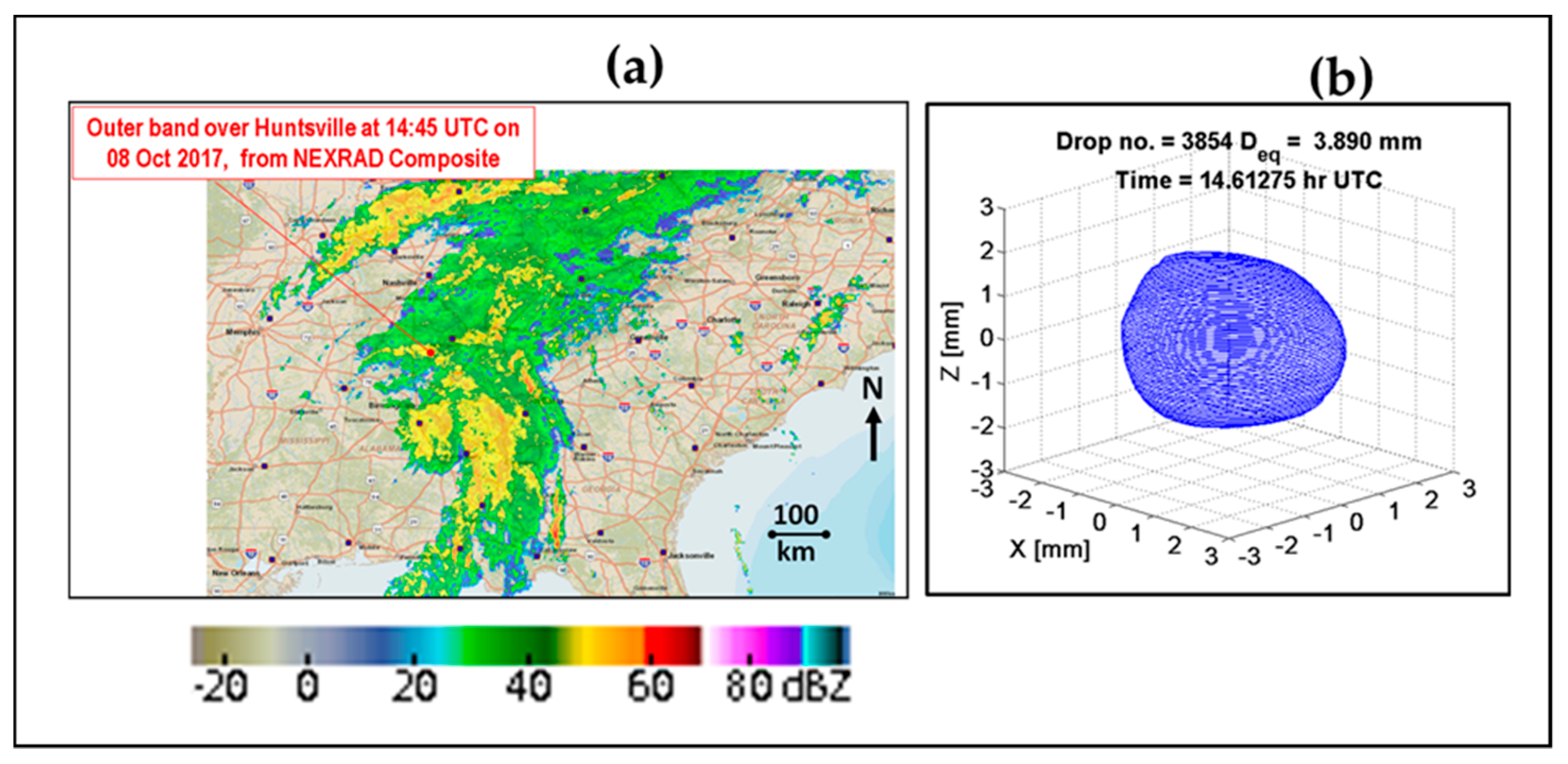
Tropical system Nate originated as a fast-moving hurricane, which made landfall on the US Gulf Coast causing storm surge, building floods, and beach erosion. More inland, Nate weakened to a tropical depression while moving north towards Northern Alabama. The rain bands lasted 18 h over the instrumented site at the University of Alabama, Huntsville (UAH), giving rise to total rain accumulation of over 31 mm. Figure 1 shows the radar mosaic image at 14:45 UTC on 08 October 2017. The surface rainfall characteristics were captured by the 2DVD [17] over the entire duration. Reflectivity data from a close by vertically pointing X-band radar (approximately 50 m from the disdrometer site), showed echo tops ranging from 1 to 4 km with pure warm rain processes being inferred when the cloud vertical extent was <3 km. At times a bright-band near 4 km height AGL during periods of heavier rain rates was observed. The red dot in Figure 1a marks the location of the instrument. A relatively large asymmetric raindrop (D_eq = 3.9 mm) is shown in panel (b).

Apart from the 2DVD, there was also another optical array probe specifically for measurement of drizzle and small drops in the range 0.1–1.5 mm (called the MPS; [18,19]). The disdrometers were complimented by collocated rain gage, wind measurements at 10-m height, and the abovementioned vertically pointing X-band Doppler radar [20] named XPR very close to the disdrometers. Rain gage data showed 1-min rates in the range 3–10 mm/h for the entire event. The temperature at 2-m height was around 73–75 °F (23–24 °C) during much of the storm period (02 to 20 h UTC). A C-band dual-polarization radar (ARMOR) [21], located 15 km from UAH made regular and frequent scans over the site.

As mentioned earlier Nate was degraded to a tropical depression soon after it made landfall on the Mississippi coast and during the movement to northern Alabama. By the time the rain bands were detected near Huntsville the 10-m sustained wind speeds measured at the instrumented site were less than 8 m/s.

3. DVD Data and Processing

The 2D-video disdrometer (2DVD) operation principles have been described in a number of previous publications [5,22,23]. It is the only disdrometer that gives the drop images in two orthogonal planes and the fall speed for each drop that falls in the 10 cm × 10 cm measurement area. Recently, the contoured shapes in the two orthogonal planes were used to derive the 3-dimensional particle shapes which have been described in [8,9,11]. The procedure involved in the drop contour derivation also includes a ‘deskewing’ technique which not only yields the corrected contoured shapes for each drop but also enables the magnitude and direction of the horizontal drop velocity to be determined. However, due to a number of limitations, such as horizontal resolution of 0.17 mm and mismatching of images (of small drops) from the 2 cameras, the velocity and shape information can only be retrieved for relatively large drops, in particular for drops with D_eq larger than 1.5 or 2 mm.

The 2DVD measurements during the entire event revealed that the drop diameters (D_eq) did not exceed 4 mm. There were 601 drops with D_eq > 2.5 mm out of 1,467,540 drops in total; out of these, only 79 drops exceeded 3 mm and only 12 drops exceeded 3.5 mm. One of the biggest drops recorded (3.9 mm) is shown in panel (b) of Figure 1 at 14:36:46 UTC. The reflectivity from the C-band ARMOR radar was about 40 dBZ at this time. A small degree of shape deformation is visible.

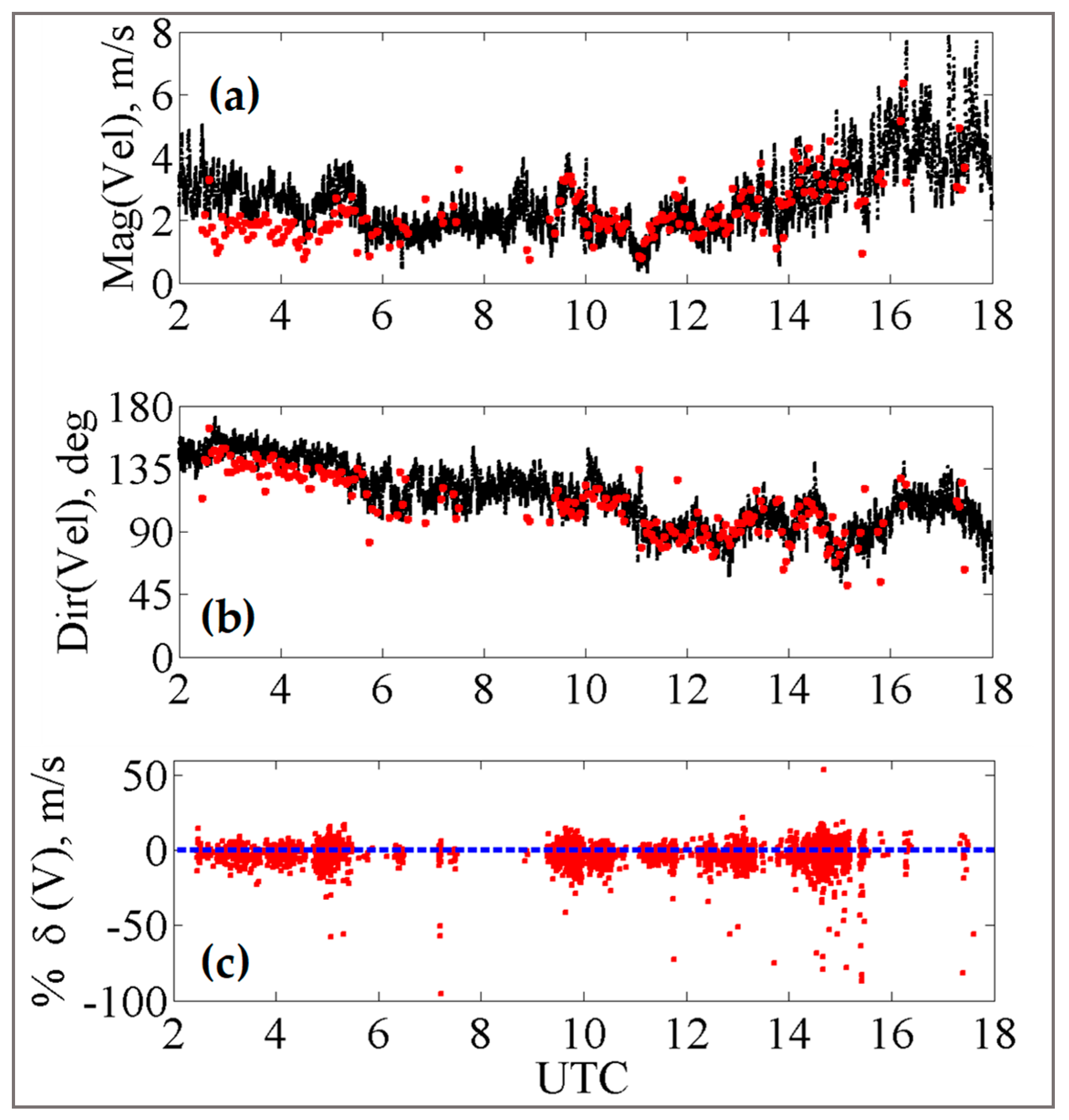
The magnitude and direction of drop horizontal velocities for all drops >2 mm derived from the 2DVD deskewing procedure are shown as red points in panels (a) and (b) of Figure 2, respectively. They are compared with anemometer measurements at 10 m height (black points) from the same location for most of the storm period (02:00 to 20:00 h UTC). Note the drop horizontal velocities were averaged over 3 min. The close agreement is consistent with the notion that the horizontal motion of the drop responds instantaneously to the horizontal wind [24]. Note that the fall speed of drop is assumed constant and is measured separately by the time taken by the drop to transit between the two light planes [17]. The measurement of horizontal drop velocity provided by the deskewing algorithm assumes that it does not change with height between the two light planes which are separated by only 6 mm and is thus independent of the fall speed measurement.

In panel (c), we show the percentage of deviation of the drop fall velocities from the expected terminal fall speeds of Gunn–Kinzer [25], again for all drops >2 mm. The zero-deviation line is marked as a dashed blue line. Fluctuations can be observed, which is to be expected, but they appear to be distributed fairly evenly around the zero-deviation line throughout the event. However, at around 15:00 UTC, a larger fraction of drops (relative to earlier times) show significantly negative percentages (<−30%) or slowing down of fall speeds relative to Gunn-Kinzer. Bringi et al. [19] observed such slowing down of mm-sized drops which was correlated with high turbulent intensities as defined in [26]. However, majority of the drops in the outer rain bands of TD Nate have fall velocities within the expected range of Gunn–Kinzer (e.g., [27] for sea level).

4. Scattering Calculations

The scattering calculations have been carried out for all 601 drops captured from the outer rain bands of TD Nate with D_eq > 2.5 mm. The simulation program used within this study is CST Microwave Studio (MWS) of the CST Studio Suite 2019. The use of this software for the scattering calculation of each individual drop has been automated. Visual Basic for Application language was used for creating structures and controlling procedures in CST MWS. In the following paragraphs the main steps of the scattering calculations are outlined.

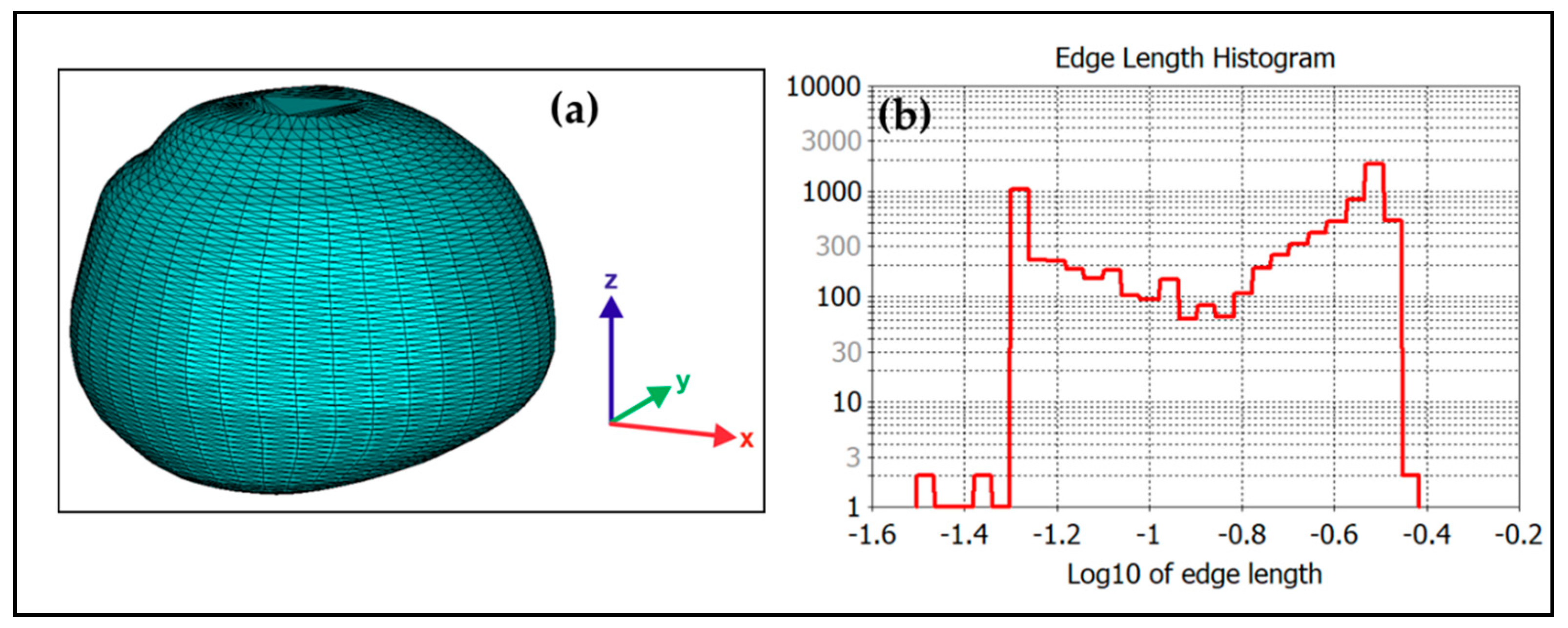
The 3D shapes of each raindrop were reconstructed with Matlab-software using the procedure described in [8,9]. For each drop a STL-file (STL for stereolithography) was generated that characterizes the surface geometry of the drop without specifying material or scale information. The STL-files of the drops were imported into CST MWS. Dielectric properties of water at a temperature of 68° F (20 °C) and a frequency of 5.625 GHz were assumed. This assumption is standard since the scattering calculations, especially the H and V-polarized radar cross-sections, are not very sensitive to water temperature. Following the model of Ray [28] this leads to a complex permittivity ε of 72.5-j22.43 (refractive index m = 8.6137-j1.3020). After importing and scaling the shape, a meshing algorithm is performed by CST MWS. Figure 3a shows the mesh of an example drop. The drop is approximated by a set of triangles that are connected by common edges or by corner points. The triangulation is based on the outer surfaces that occur when reconstructing the drop. The 3D reconstruction is carried out with an angular resolution of 10 degrees in azimuth and with 0.05 mm vertical resolution. If a drop, for example, has a height of 3 mm this procedure leads to approximately 36 × (3/0.05) = 2160 quadrangular planar surfaces on the outside. As each surface is split in order to form triangles, the number of surfaces duplicates.

Figure 3b shows the histogram of the edge length of the triangulation of the drop shown in Figure 3a. For the given drop the shortest edge length is ~0.03 mm and the largest edge length is ~0.37 mm. On average the edge length is 0.1 mm. The largest detected drops with an equal volume diameter of ~3.8 mm are approximated by more than 5000 triangles. Given a frequency of 5.626 GHz and therefore a wavelength of 5.3 cm, each drop is modelled with at least 15 grid points per wavelength.

A plane wave excitation source was defined with linear polarization and a frequency of 5.625 GHz. The Radar Cross Section (RCS) of each individual drop was calculated for both horizontal and vertical polarization using the CST Integral Equation Solver which is suitable for electrically large dielectric objects (size is large compared to wavelength).

5. Results for Individual Particles

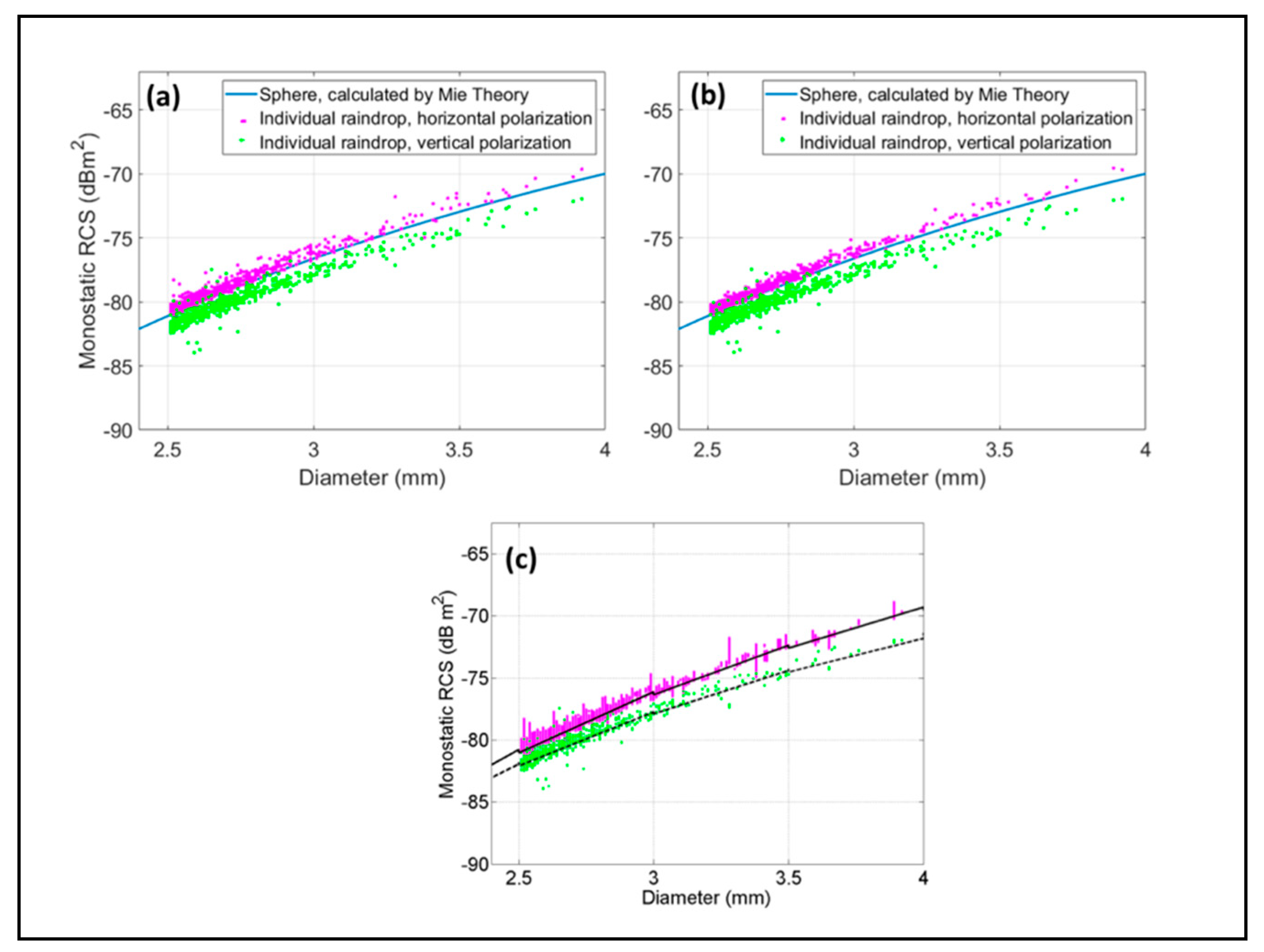
RCS calculations were carried out for 0° to 359° angles with 1° step size, in order to cover all possible look angles (i.e., the azimuthal angle φ) in the horizontal plane. To ensure plausibility of the results, the calculated RCS of all 601 individual drops were compared to the respective values of equal-volume spheres. Figure 4 illustrates the RCS in terms of the equi-volume drop diameter for one defined view angle in panel (a) as well as for the averaged RCS over all orientations within 360° in panel (b). The figures show that the modelled shape can differ by ± 3 dB from a sphere representation.

Panel (c) shows the same points as panel (b) for H and V polarizations for all look angles, but here we have superimposed two curves which represent the RCS variation when a fixed shape-size relationship is used, in this case, the oblate-spheroid approximation of the Beard–Chuang [2] shapes (henceforth the BC model which is based on a balance between aerodynamic, gravitational and surface tension forces). The curves are shown as black solid line for H polarization and black dashed line as V polarization. All variations show a general increase in RCS with drop diameter, at least up to 4 mm. Since the shape is fixed for a given drop size, the scattering amplitude will be expected to be a single curve for a given polarization. Furthermore, the rotational symmetry of the drop shape will result in RCS being independent of the look angle. The scatter in the RCS values for the reconstructed drops is of course due to both variation in shapes and the variation with look angle, but even so they appear to lie evenly scattered on both sides of the two (solid black and dashed black) curves.

The differential reflectivity of each reconstructed drop is obtained from the difference between the horizontal and vertical polarization radar cross-sections. Because both the H and V radar cross sections for any given drop will vary with the look angle, its differential reflectivity will also have a φ variation. This has been illustrated in [11] in terms of the complex scattering amplitudes for both polarizations (see their Figure 7 where φ was varied from 0 to 360° in the horizontal plane).

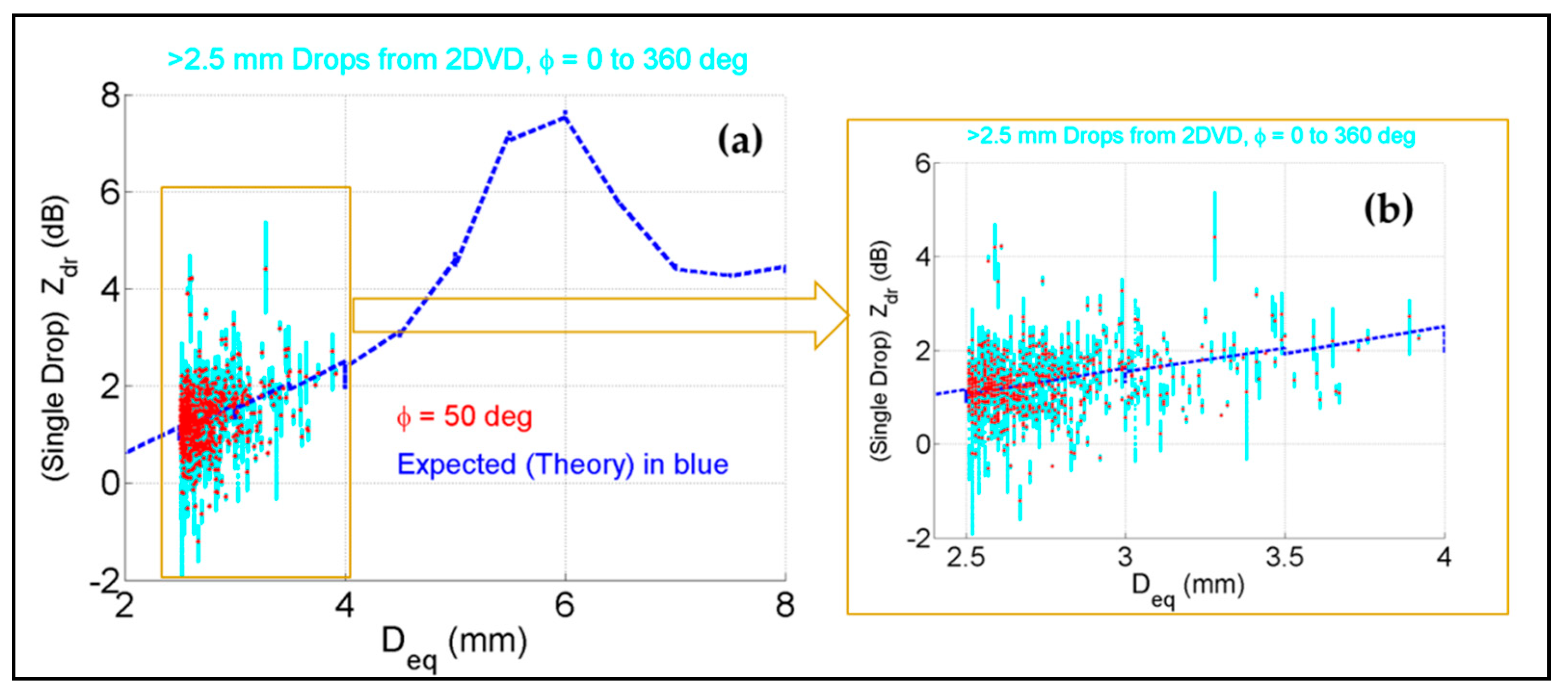
The overall variation of Z_dr with drop diameter for all the 601 drops is shown in panel (a) of Figure 5 as cyan color points. For comparison, the theoretical curve (using the T-matrix code) assuming the BC model is included (as the blue dotted line). The zoomed in version for D_eq up to 4 mm is shown in panel (b) for more clarity. In both cases, the cyan points encompass the full range of φ from 0 to 360°. Superimposed on the plots are red points which correspond to φ = 50°, which in fact is close to the look angle (i.e., azimuth) from the ARMOR radar site to the 2DVD location.

From Figure 5, certain observations can be made:

(i)

Compared to the Z_dr from T-matrix based on the BC model, the Z_dr values for individual drops can differ by several dB indicating shape deviations from BC (which is an equilibrium shape model).

(ii)

The majority of the deviations span both positive and negative values, implying the drop shapes can be ‘elongated’ either in the horizontal plane or along the vertical, due to drop oscillations (including mixed-mode).

(iii)

The φ = 50° points show less scatter than the φ = 0 to 360° (cyan) points; this is to be expected.

(iv)

The resonance region around D_eq = 6 mm will not have any implications for the outer rain bands of TD Nate since all drops recorded were <4 mm.

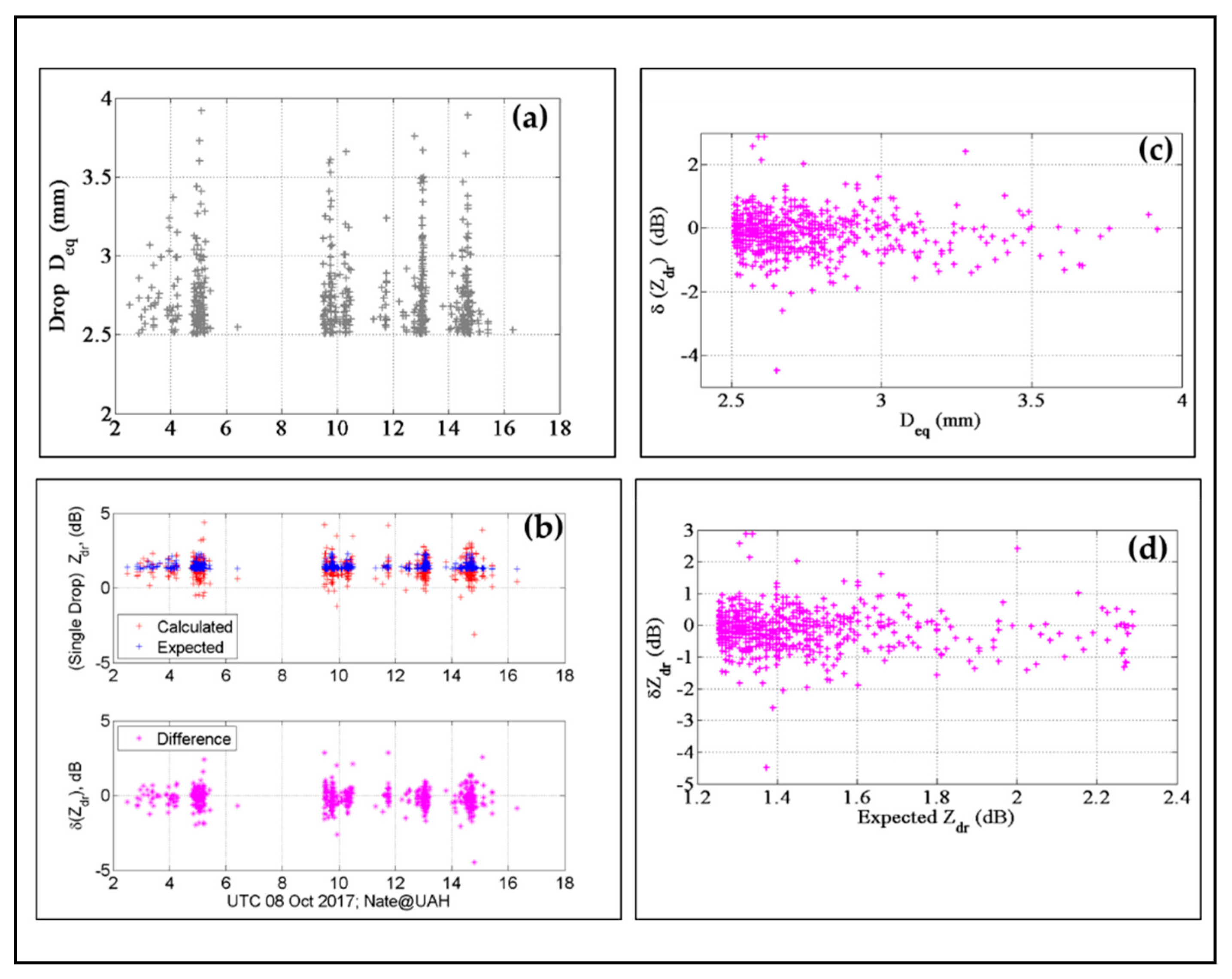
Figure 6 summarizes the variation of Z_dr as function of each drop >2.5 mm during the event. Panel (a) shows the time series of drop sizes. Panel (b) shows the corresponding Z_dr of each drop based on the 2DVD-reconstructed shape and the CST integral equation solver (this is referred to as the calculated Z_dr in panel b). The expected value of Z_dr for each drop is based on the oblate shape axis ratio versus D_eq model of [5]. Panel (c) shows the difference between the calculated and expected values, which can be denoted as δ(Z_dr) = Z_dr [from drop-by-drop 3D-reconstructed shape] minus Z_dr [from drop-by-drop mean oblate shape]. Panel (d, e) show, respectively, the scatter plot of δ(Z_dr) versus D_eq and δ(Z_dr) versus the expected value of Z_dr.

Once again, we summarize the important observations:

(i)

The outer rain bands of TD Nate did not produce drops larger than 4 mm over Huntsville (as mentioned earlier);

(ii)

The δ(Z_dr) can be significant, but overall, they tend to be distributed evenly around 0 dB. For the larger drops (>3 mm), δ(Z_dr) showed a tendency to be slightly more negative, i.e., drops being somewhat closer to spherical in shape;

(iii)

The skewness towards negative δ(Z_dr) values were more apparent just prior to 15:00 UTC when the wind speeds were seen to increase and the change in wind direction was more rapid. It was around this time that the fall velocities also showed a small but noticeable number of drops having lower than expected velocities.

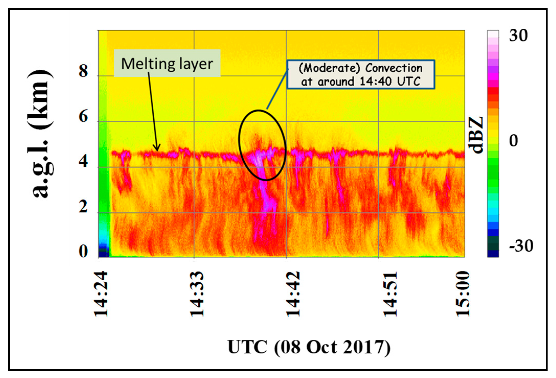
The vertically-pointing X-band Doppler with its high range resolution provided details of the reflectivity height profiles as a time series (see Figure 7 which gives a zoomed in view from 14:24–15:00 UTC). The highest reflectivity in the bright-band occurred at 14:40 with frequent visually observable streaks of reflectivity penetrating upwards of the bright-band, especially at 14:40. According to Fabry and Zawadzki [29], these pockets or streaks might indicate updrafts (their Figure 11b) and rimed particles (graupel). There appears to be a correlation between the occurrence of vertical air motion at 14:40 and significant negative values (~−2 dB) of δ(Z_dr) and slowing down of the fall velocities (relative to terminal speeds) at the surface. This correlation is speculative as there are no studies linking vertical air motion and riming above the bright-band to drop shapes and fall velocities near the surface.

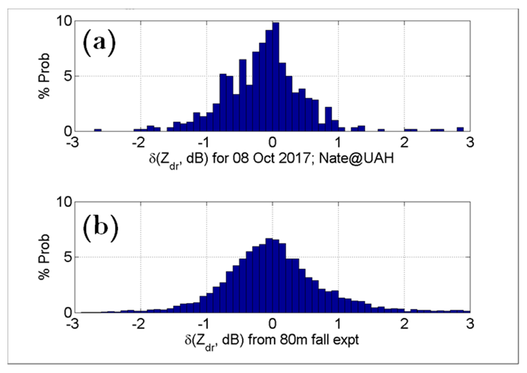
The histogram of δ(Z_dr) for D_eq > 2.5 mm for the outer rain bands is shown in Figure 8a. The mode of the distribution lies very close to 0 dB. Significantly more negative δ(Z_dr) were observed, compared with positive δ(Z_dr). To quantify this, as an example, 149 drops out of 601 drops had δ(Z_dr) less than −0.5 dB whereas only 72 drops had δ(Z_dr) greater than 0.5 dB. Recall that δ(Z_dr) is the difference between Z_dr from 3D-reconstructed drop shapes and the Z_dr from oblate axis ratio versus D_eq model given in [5]. For example, consider the extreme case where δ(Z_dr) for all drops were negative, i.e., more spherical on average. Further, if the algorithm for retrieval of D_m (mass-weighted mean diameter) from Z_dr were derived based on expected oblate axis ratio model of Thurai et al. alone, then the D_m would be biased too high for the measured Z_dr, and for a given reflectivity, the rain rates would be biased too low [1]. In our case the mode of the distribution is close to 0 dB but visually the distribution is negatively skewed (Figure 8a). By way of comparison, panel (b) shows the δ(Z_dr) histogram derived from the 80 m fall artificial rain experiment ([4,5]), where only 5% of the measured drops were found to have significant asymmetry. In the latter experiment, the axis ratio of each drop was calculated as the ratio of the vertical chord to the horizontal chord (chord is a line segment joining any two points on a curve) The Z_dr for each drop was then estimated using the relation from Jameson [30]:

$${10}^{-0.1\left({\mathrm{Z}}_{\mathrm{dr}}\right)}={\left(\frac{\mathrm{a}}{\mathrm{b}}\right)}^{\frac{7}{3}}$$

(1)

which is accurate for axis ratios >0.5 for oblates and <1.5 for prolates. The Z_dr from (1) is defined as the calculated value. Note that the axis ratio distribution reflects drop oscillations in the 80 m fall experiment. The expected value of Z_dr for each drop is (as before) based on the oblate shape axis ratio versus D_eq model of [5]. The motivation to compare the histograms in this manner is that the 80 m fall experiment can be considered as a baseline for axis ratio distributions for drops <9 mm in very light wind conditions. Whereas the outer bands of TD Nate had D_eq < 4 mm under higher wind conditions (speeds ~8 m/s). It is useful to know that the mode of the histograms is close to 0 dB implying that the most probable axis ratios are not very different between the natural rain event and the artificial rain experiment. The width of the histogram in Figure 8b seems larger than that in Figure 8a which might be due to much larger drops in the artificial rain experiment with correspondingly larger oscillation amplitudes ([4,5]). Finally, the slight negative skewness in Figure 8a indicates a higher proportion of asymmetric drops as mentioned above.

6. One-Minute Based Z_h, Z_dr Calculations and Comparisons with ARMOR

To compute the reflectivity from the individual scattering amplitudes, for example over a 1-min period, we perform drop-by-drop integration of the radar cross-sections (strictly speaking the covariance matrix elements) during that time period. If we denote the H-polarization reflectivity for the ith drop as z_i^h, then the overall reflectivity from all drops over the 1-min period is given by:

$${\mathrm{Z}}_{\mathrm{h}}=\frac{1}{\mathrm{A}\Delta \mathrm{t}}{\displaystyle {\displaystyle \sum }_{\mathrm{i}=1}^{\mathrm{n}}}{\mathrm{v}}_{\mathrm{i}}^{-1}{\mathrm{z}}_{\mathrm{i}}^{\mathrm{h}}$$

(2)

where A is the measurement area of the 2DVD, Δt is the averaging time period, and v_i is the vertical velocity of the ith drop. For V polarization, similar integration is performed using the corresponding RCS values, z_i^v. Both are converted to the conventional dBZ units and Z_dr for that 1-min period is determined from the difference between the two.

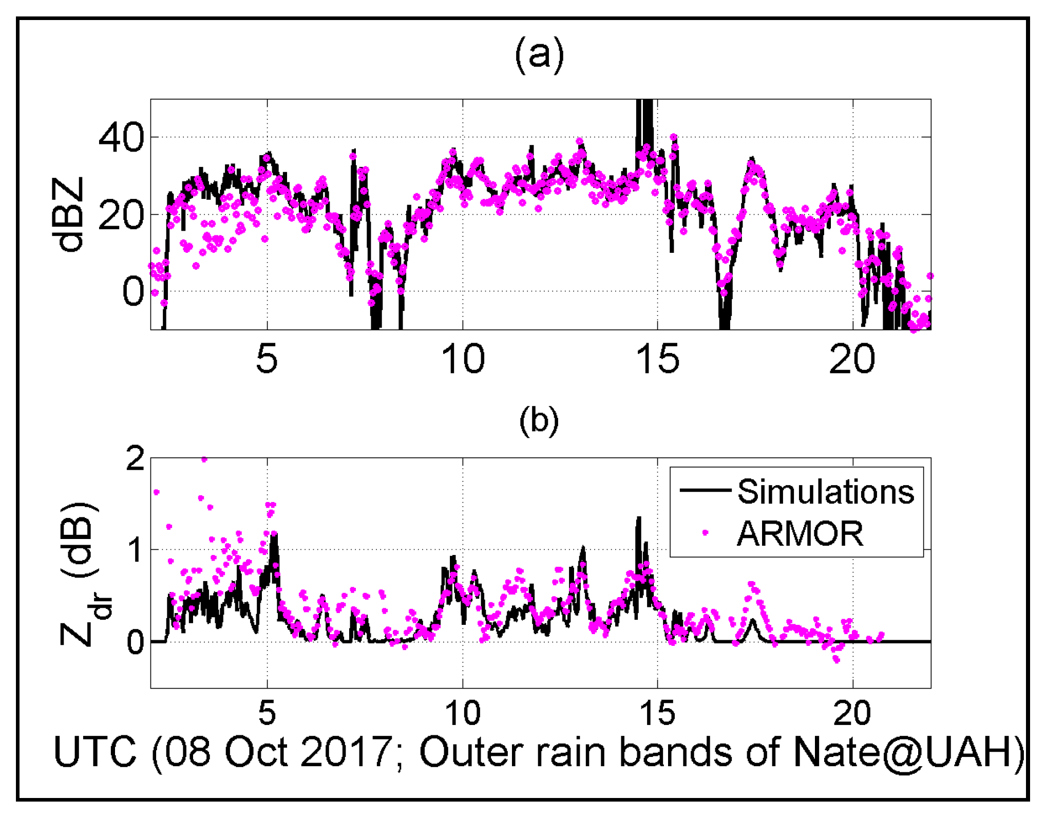
The 1-min based calculations for the entire 18 h event period is shown in Figure 9 and compared with the C-band ARMOR radar data over and in the vicinity of the disdrometer site. The radar data were extracted from low elevation (0.7°) PPI sweeps every few 2–3 min. The resolution volumes were selected from 9 range bins km surrounding the 2DVD location. The height of the selected pixels is 183 m above ground level. Time series of the averaged reflectivity and Z_dr were further smoothed over 3 consecutive points. Panel (a) shows the Z comparison, and panel (b) the Z_dr comparison. After 05:00, there is excellent agreement in both cases. Prior to 05:00, radar Z appears to be somewhat lower than the simulations and the Z_dr slightly higher. It was around this time that the retrieved horizontal drop velocities (from 2DVD measurements) showed some discrepancy with the wind sensor data. Hence it is possible that the shape reconstruction is not precise enough to provide sufficiently accurate scattering amplitudes. It is not possible to consider all the factors that might have led to the discrepancy since simulated reflectivity is overestimated and the Z_dr is underestimated relative to radar measurements (i.e., opposite directions). The dependence of reflectivity on drop shapes should be minor so the simulated Z_h could be more a result of 2DVD-based sizing while the underestimation of Z_dr could be more related to 3D-reconstruction errors.

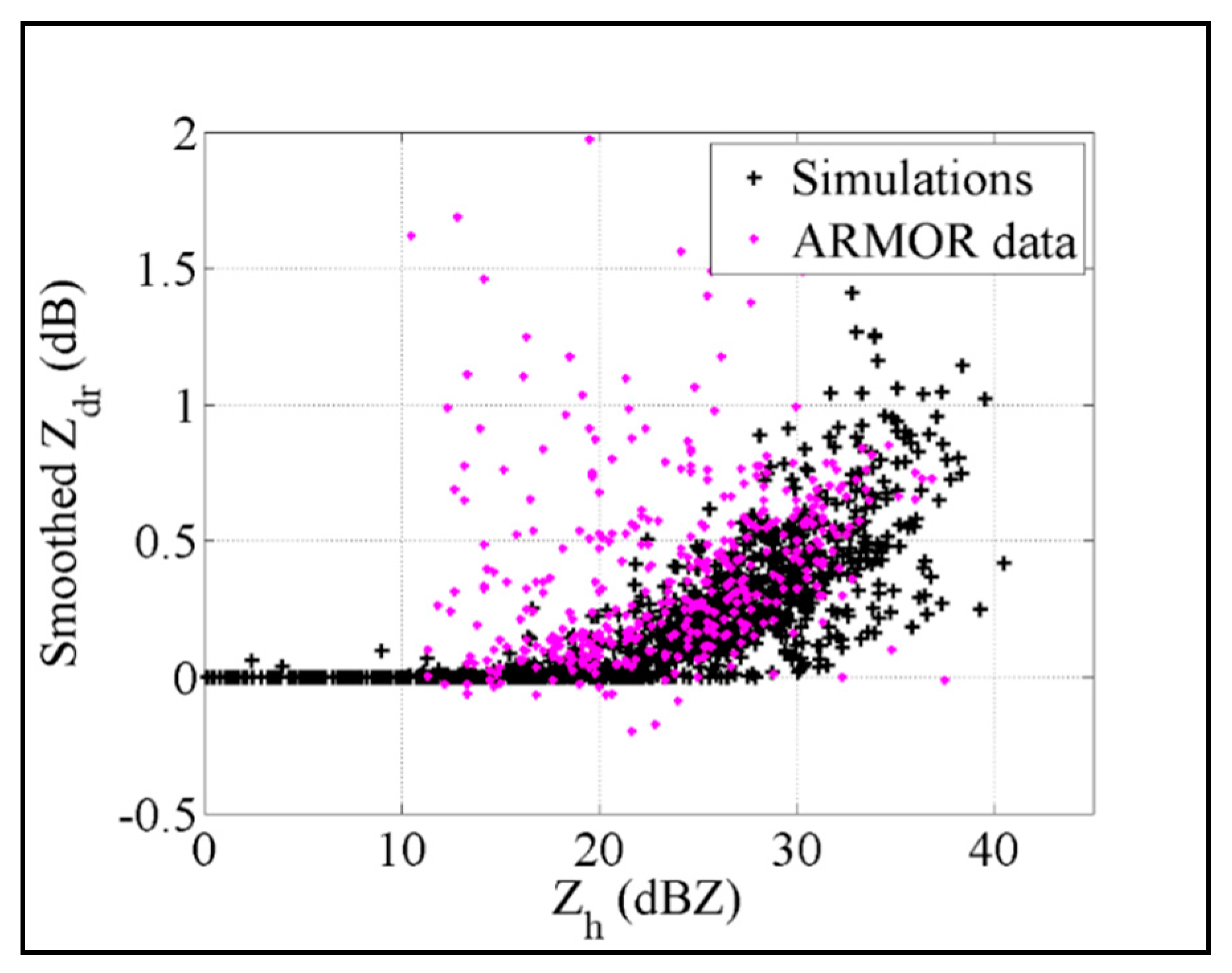
The Z_dr versus Z_h variation from the CST simulations for 05:00–20:00 are compared with those from the radar observations in Figure 10. The variations are in good agreement with each other and both show a clear increase of Z_dr with increasing Z_h beyond 22 dBZ. On average the variation of Zdr versus Z is close to that obtained by Wang et al. [31] based on S-band WSR−88D measurements for stratiform rain for Z > 30 dBZ and closer to tropical rain for Z < 25 dBZ (their Figure 3). This is reasonable since the outer rain bands probably lie between these two rain types. Note also the maximum reflectivity values for both cases [31] did not go beyond 40 dBZ and the maximum Z_dr did not go beyond 1.5 dB. All these features provide confirmation and validation for the drop-by-drop based scattering calculations.

7. Conclusions

The analyses of the 2DVD measurements during the outer bands of tropical depression Nate over HSV and the scattering calculations are summarized below:

(i)

The horizontal velocity of the drops deduced from the 2DVD is close to the horizontal wind velocity, both in terms of magnitude and direction. This implies that deskewing can be done for drops that do not have an axis of symmetry, using horizontal wind data preferably at the 2DVD sensor height above ground.

(ii)

The Z_dr calculated for the 3D-reconstructed drops (drop-by-drop calculations) showed substantial scatter, mainly from the azimuthal variation or look angle. The scatter reduced considerably when the look angle corresponding to the 2DVD camera viewing direction was used. On average, the Z_dr from the 3D-reconstructed shapes were in good agreement with the Z_dr based on the BC model (though drop-by-drop deviations in Z_dr do occur).

(iii)

The histogram of δ(Z_dr) from the rain bands of TD Nate and the 80-m fall artificial rain experiment were compared. Both histograms had a mode at 0 dB implying that the most probable axis ratios are not very different between the natural rain event and the artificial rain experiment. However, the histogram corresponding to the rain bands of TD Nate was negatively skewed and with smaller width compared to the 80-m fall experiment. The slight negative skewness indicates a higher proportion of asymmetric drops as mentioned above while the smaller width is likely a result of the maximum D_eq< 4 mm (compared with D_eq < 9 mm for the artificial rain experiment).

(iv)

The Z and Z_dr calculated using the individual C-band scattering amplitudes of each drop over 1-min interval shows, in general, excellent agreement with the C-band radar observations over the disdrometer for the entire 18 h period of the outer rain bands of TD Nate in Huntsville. On average the Z_dr values for a given interval of Z are consistent with rain type being stratiform-tropical.

Regarding (i), even though it is assumed (e.g., [24]) that horizontal velocities of precipitation particles do not differ from prevalent wind velocities (e.g., [24,32]) during steady conditions, it is only the 2DVD instrument which is capable of providing direct observational evidence of this in natural rain. It is consistent with previous studies [11,33] from a line convection event and a hurricane event which showed excellent agreement of the 2DVD-based drop horizontal velocities at near-ground level with the wind measurements at 10 m height. Currently, a 3D sonic anemometer has been installed at the UAH site to measure the ambient winds and turbulent intensity

The scattering models in current use typically assume mean axis ratio of oblate drops versus D_eq relations (either the BC equilibrium model [2], or [5] or empirical fit given in [34]) together with Gaussian canting angle distribution [35] for simulating polarimetric radar observables. Here, we use a higher order simulation based on scattering from 3D-reconstructed shapes and drop-by-drop integration which is possible with recent advances in 2DVD data processing. In the simulations of Z_dr for the rain bands of TD Nate, the drop-by-drop approach on average gave similar values as using the “bulk” assumptions mentioned above. Several other event analyses have also shown this to be the case [12]. For strong convective rain with large drops, which are associated with high wind speeds and/or rapid change in wind direction, the drop-by-drop approach is preferred over the “bulk” approach as the former accounts for the variance in shapes (the orientation variance is built-in), which are important for other dual-polarization variables such as the copolar correlation coefficient and depolarization ratios [12].

References

- Bringi, V.N.; Chandrasekar, V. Polarimetric Doppler Weather Radar; Cambridge University Press: Cambridge, UK, 2001. [Google Scholar]
- Beard, K.V.; Chuang, C. A new model for the equilibrium shape of raindrops. J. Atmos. Sci. 1987, 44, 1509–1524. [Google Scholar] [CrossRef]
- Szakáll, M.; Diehl, K.; Mitra, S.K.; Borrmann, S. A wind tunnel study on the shape, oscillation, and internal circulation of large raindrops with sizes between 2.5 and 7.5 mm. J. Atmos. Sci. 2009, 66, 755–765. [Google Scholar] [CrossRef]
- Thurai, M.; Bringi, V.N. Drop axis ratios from a 2D video disdrometer. J. Atmos. Ocean. Technol. 2005, 22, 966–978. [Google Scholar] [CrossRef]
- Thurai, M.; Huang, G.-J.; Bringi, V.N.; Randeu, W.L.; Schönhuber, M. Drop shapes, model comparisons, and calculations of polarimetric radar parameters in rain. J. Atmos. Ocean. Technol. 2007, 24, 1019–1032. [Google Scholar] [CrossRef]
- Thurai, M.; Bringi, V.N.; Szakáll, M.; Mitra, S.K.; Beard, K.V.; Borrmann, S. Drop shapes and axis ratio distributions: Comparison between 2D video disdrometer and wind-tunnel measurements. J. Atmos. Ocean. Technol. 2009, 26, 1427–1432. [Google Scholar] [CrossRef]
- Beard, K.V. Oscillation modes for predicting raindrop axis and back scatter ratios. Radio Sci. 1984, 19, 67–74. [Google Scholar] [CrossRef]
- Schönhuber, M.; Schwinzerl, M.; Lammer, G. 3D reconstruction of 2DVD-measured raindrops for precise prediction of propagation parameters. In Proceedings of the 10th European Conference on Antennas and Propagation (EuCAP), Davos, Switzerland, 10–15 April 2016; pp. 3403–3406. [Google Scholar] [CrossRef]
- Schwinzerl, M.; Schönhuber, M.; Lammer, G.; Thurai, M. 3D reconstruction of individual raindrops from precise ground-based precipitation measurements. EMS Annu. Meet. Abstr. 2016, 13, EMS2016-601. [Google Scholar]
- Chobanyan, E.N.; Šekeljić, N.; Manic, A.B.; Ilić, M.M.; Bringi, V.N.; Notaroš, B.M. Efficient and accurate computational electromagnetics approach to precipitation particle scattering analysis based on higher-order method of moments integral equation modeling. J. Atmos. Ocean. Technol. 2015, 32, 1745–1758. [Google Scholar] [CrossRef]
- Thurai, M.; Manić, S.B.; Schönhuber, M.; Bringi, V.N.; Notaroš, B.M. Scattering calculations at C-band for asymmetric raindrops reconstructed from 2D video disdrometer measurements. J. Atmos. Ocean. Technol. 2017, 34, 765–776. [Google Scholar] [CrossRef]
- Manić, S.B.; Thurai, M.; Bringi, V.N.; Notaroš, B.M. Scattering Calculations for Asymmetric Raindrops during a Line Convection Event: Comparison with Radar Measurements. J. Atmos. Ocean. Technol. 2018, 35, 1169–1180. [Google Scholar] [CrossRef]
- Thurai, M.; Bringi, V.N.; Petersen, W.A.; Gatlin, P.N. Drop shapes and fall speeds in rain: Two contrasting examples. J. Appl. Meteor. Climatol. 2013, 52, 2567–2581. [Google Scholar] [CrossRef]
- Kirstetter, P.E.; Gourley, J.J.; Hong, Y.; Zhang, J.; Moazamigoodarzi, S.; Langston, C.; Arthur, A. Probabilistic precipitation rate estimates with ground-based radar networks. Water Resour. Res. 2015, 51, 1422–1442. [Google Scholar] [CrossRef]
- Rasmussen, R.M.; Heymsfield, A.J. Melting and Shedding of Graupel and Hail. Part I: Model Physics. J. Atmos. Sci. 1987, 44, 2754–2763. [Google Scholar] [CrossRef] [Green Version]
- Bringi, V.N.; Rasmussen, R.M.; Vivekanandan, J. Multiparameter Radar Measurements in Colorado Convective Storms. Part I: Graupel Melting Studies. J. Atmos. Sci. 1986, 43, 2545–2563. [Google Scholar] [CrossRef] [Green Version]
- Schönhuber, M.; Lammer, G.; Randeu, W.L. The 2D-video-disdrometer. In Precipitation: Advances in Measurement, Estimation and Prediction; Michaelides, S.C., Ed.; Springer: New York, NY, USA, 2008; pp. 3–31. [Google Scholar]
- Baumgardner, D.; Kok, G.; Dawson, W.; O’Connor, D.; Newton, R. A new ground-based precipitation spectrometer: The Meteorological Particle Sensor (MPS). In Proceedings of the 11th Conference on Cloud Physics, Ogden, UT, USA, 3–7 June 2002. paper 8.6. [Google Scholar]
- Bringi, V.N.; Thurai, M.; Baumgardner, D. Raindrop fall velocities from an optical array probe and 2-D video disdrometer. Atmos. Meas. Tech. 2018, 11, 1377–1384. [Google Scholar] [CrossRef] [Green Version]
- Hulsey, C.B.; Knupp, K. An Analysis of a Mesoscale Features during IOP 4C of the VORTEX-SE Field Campaign. In Proceedings of the 97th American Meteorological Society Annual Meeting, Seattle, WA, USA, 22–26 January 2017. [Google Scholar]
- Petersen, W.A.; Knupp, K.R.; Cecil, D.J.; Mecikalski, J.R. The University of Alabama Huntsville THOR Center instrumentation: Research and operational collaboration. In Proceedings of the 33rd International Conference on Radar Meteorology, Cairns, Queensland, Australia, 6–10 August 2007; paper 5.1. Available online: https://ams.confex.com/ams/33Radar/webprogram/Paper123410.html (accessed on 18 January 2020).
- Schönhuber, M.; Randeu, W.L.; Urban, H.E.; Poiares Baptista, J.P.V. Field measurements of raindrop orientation angles. In Proceedings of the AP2000 Millennium Conference on Antennas and Propagation, Davos, Switzerland, 9–14 April 2000. [Google Scholar]
- Gimpl, J. Optimised Algorithms for 2d-Video-Distrometer Data Analysis and Interpretation. Diploma Thesis, Institute of Communications and Wave Propagation, Graz University of Technology, Graz, Austria, 2003; p. 111. [Google Scholar]
- Dawson, D.T.; Mansell, E.R.; Kumjian, M.R. Does Wind Shear Cause Hydrometeor Size Sorting? J. Atmos. Sci. 2015, 72, 340–348. [Google Scholar] [CrossRef]
- Gunn, R.; Kinzer, G.D. The terminal velocity of fall for water droplets in stagnant air. J. Meteorol. 1949, 6, 243–248. [Google Scholar] [CrossRef] [Green Version]
- Garrett, T.J.; Yuter, S.E. Observed influence of riming, temperature, and turbulence on the fallspeed of solid precipitation. Geophys. Res. Lett. 2014, 41, 6515–6522. [Google Scholar] [CrossRef]
- Atlas, D.; Srivastava, R.C.; Sekhon, R.S. Doppler radar characteristics of precipitation at vertical incidence. Rev. Geophys. 1973, 11, 1–35. [Google Scholar] [CrossRef]
- Ray, P. Broadband complex refractive indices of ice and water. Appl. Opt. 1972, 11, 1836–1844. [Google Scholar] [CrossRef]
- Fabry, F.; Zawadzki, I. Long-Term Radar Observations of the Melting Layer of Precipitation and Their Interpretation. J. Atmos. Sci. 1995, 52, 838–851. [Google Scholar] [CrossRef]
- Jameson, A.R. Microphysical interpretation of multiparameter radarmeasurements in rain. Part I: Interpretation of polarization measure-ments and estimation of raindrop shapes. J. Atmos. Sci. 1983, 40, 1792–1802. [Google Scholar] [CrossRef] [Green Version]
- Wang, Y.; Cocks, S.; Tang, L.; Ryzhkov, A.; Zhang, P.; Zhang, J.; Howard, K. A Prototype Quantitative Precipitation Estimation Algorithm for Operational S-Band Polarimetric Radar Utilizing Specific Attenuation and Specific Differential Phase. Part I: Algorithm Description. J. Hydrometeor. 2019, 20, 985–997. [Google Scholar] [CrossRef]
- Marshall, J.S. Precipitation trajectories and patterns. J. Meteor. 1953, 10, 25–29. [Google Scholar] [CrossRef] [Green Version]
- Thurai, M.; Schönhuber, M.; Lammer, G.; Bringi, V.N. Raindrop shapes and fall velocities in “turbulent times”. Adv. Sci. Res. 2019, 16, 95–101. [Google Scholar] [CrossRef]
- Brandes, E.A.; Zhang, G.; Vivekanandan, J. Experiments in rainfall estimation with a polarimetric radar in a subtropical environment. J. Appl. Meteor. 2002, 41, 674–685. [Google Scholar] [CrossRef] [Green Version]
- Huang, G.; Bringi, V.N.; Thurai, M. Orientation Angle Distributions of Drops after an 80-m Fall Using a 2D Video Disdrometer. J. Atmos. Oceanic Technol. 2008, 25, 1717–1723. [Google Scholar] [CrossRef]
Figure 1.
(a) Composite next generation radar (NEXRAD) radar image of reflectivity during Tropical Depression Nate over Alabama on 08 October 2017 at 14:45 UTC. The location of the 2D-video disdrometer (2DVD) and other instruments is marked with a red dot; (b) shape of a large drop recorded by the 2DVD at this time (using the 3D reconstruction procedure, see Section 3).
Figure 2.
(a) Wind speed and, (b) wind direction (as black points) from the anemometer at 10 m height at the 2DVD location, respectively, along with the retrieved drop horizontal velocities from the 2DVD in red for Deq > 2 mm averaged over 3 min; (c) percentage change in the drop fall velocities from the 2DVD compared with Gunn–Kinzer.
Figure 3.
(a) Triangle mesh of an individual drop imported into CST Microwave Studio; (b) histogram of the edge length of the triangulation.
Figure 4.
Radar Cross Section (RCS) of 601 reconstructed raindrops for horizontal and vertical polarization, as a function of their respective equal volume diameter. For comparison, the RCS of a sphere is shown. f = 5.625 GHz and the refractive index m = 8.6137-j1.3020. Panel (a) is for a fixed view angle of φ = 0, and panel (b) is the averaged value of the RCS over φ = 0 to 359°. Panel (c) shows the same RCS versus Deq as panel (b) for the reconstructed drops for H and V polarizations, compared with those assuming the BC model is included (solid line, respectively, dashed line are for H,V polarizations).
Figure 5.
(a) Single drop Zdr versus Deq for the reconstructed drops for all φ angles in cyan and for φ = 50° in red, together with those for the Beard–Chuang (BC) model (dashed line in blue) using T-matrix; (b) same as panel (a) but zoomed in to cover the brown dotted line box.
Figure 6.
(a) Diameters of all drops >2.5 mm recorded during the passage of the outer rain bands of tropical depression (TD) Nate over the 2DVD; (b) (top panel) the calculated Zdr for each 3D-reconstructed drop in red and the expected Zdr for each drop (in blue), assuming the oblate axis ratio of Thurai et al., and δZ(dr) for each particle (bottom panel); (c) δ(Zdr) versus Deq; (d) δ(Zdr) versus the expected Zdr.
Figure 7.
Time series of vertical profiles of reflectivity from the vertically pointing XPR observations for 14:24 to 15:00 UTC on 08 October 2017.
Figure 8.
Histograms of δ(Zdr) for all >2.5 mm drops (a) for the reconstructed drops from the outer rain bands of TD Nate and (b) for drops recorded during the 80 m fall experiment [4] using Equation (1).
Figure 9.
(a) Reflectivity and (b) Zdr calculations derived from the individual drop scattering amplitudes using the 2DVD measurements (in black) compared with the C-band dual-polarization radar (ARMOR) radar measurements (magenta) over the 2DVD site. For the former, 1-min time interval is used.
Figure 10.
Z versus Zdr corresponding to Figure 9.
© 2020 by the authors. Licensee MDPI, Basel, Switzerland. This article is an open access article distributed under the terms and conditions of the Creative Commons Attribution (CC BY) license (http://creativecommons.org/licenses/by/4.0/).
Share and Cite
MDPI and ACS Style
Thurai, M.; Steger, S.; Teschl, F.; Schönhuber, M. Analysis of Raindrop Shapes and Scattering Calculations: The Outer Rain Bands of Tropical Depression Nate. Atmosphere 2020, 11, 114. https://doi.org/10.3390/atmos11010114
AMA Style
Thurai M, Steger S, Teschl F, Schönhuber M. Analysis of Raindrop Shapes and Scattering Calculations: The Outer Rain Bands of Tropical Depression Nate. Atmosphere. 2020; 11(1):114. https://doi.org/10.3390/atmos11010114
Chicago/Turabian StyleThurai, Merhala, Sophie Steger, Franz Teschl, and Michael Schönhuber. 2020. "Analysis of Raindrop Shapes and Scattering Calculations: The Outer Rain Bands of Tropical Depression Nate" Atmosphere 11, no. 1: 114. https://doi.org/10.3390/atmos11010114
Note that from the first issue of 2016, this journal uses article numbers instead of page numbers. See further details here.