Turbulence, Low-Level Jets, and Waves in the Tyrrhenian Coastal Zone as Shown by Sodar
by
 ,
,
Igor Petenko
1,2,* ,
,
Giampietro Casasanta
1, 
Simone Bucci
3, 
Margarita Kallistratova
2,
Roberto Sozzi
4 and
Stefania Argentini
1 
1
CNR-ISAC—Italian National Research Council, Institute of Atmospheric Science and Climate, 00133 Rome, Italy
2
A.M. Obukhov Institute of Atmospheric Physics, Russian Academy of Sciences, Moscow 119017, Russia
3
Serco S.p.A., 00044 Frascati, Italy
4
ARIANET S.r.l., 20128 Milan, Italy
*
Author to whom correspondence should be addressed.
Atmosphere 2020, 11(1), 28; https://doi.org/10.3390/atmos11010028
Submission received: 18 October 2019
/
Revised: 13 December 2019
/
Accepted: 23 December 2019
/
Published: 27 December 2019
(This article belongs to the Special Issue Vertical Structure of the Atmospheric Boundary Layer in Coastal Zone)
Abstract
:The characteristics of the vertical and temporal structure of the coastal atmospheric boundary layer are variable for different sites and are often not well known. Continuous monitoring of the atmospheric boundary layer was carried out close to the Tyrrhenian Sea, near Tarquinia (Italy), in 2015–2017. A ground-based remote sensing instrument (triaxial Doppler sodar) and in situ sensors (meteorological station, ultrasonic anemometer/thermometer, and net radiometer) were used to measure vertical wind velocity profiles, the thermal structure of the atmosphere, the height of the turbulent layer, turbulent heat and momentum fluxes in the surface layer, atmospheric radiation, and precipitation. Diurnal alternation of the atmospheric stability types governed by the solar cycle coupled with local sea/land breeze circulation processes is found to be variable and is classified into several main regimes. Low-level jets (LLJ) at heights of 100–300 m above the surface with maximum wind speed in the range of 5–18 m s−1 occur in land breezes, both during the night and early in the morning. Empirical relationships between the LLJ core wind speed characteristics and those near the surface are obtained. Two separated turbulent sub-layers, both below and above the LLJ core, are often observed, with the upper layer extending up to 400–600 m. Kelvin–Helmholtz billows associated with internal gravity–shear waves occurring in these layers present opposite slopes, in correspondence with the sign of vertical wind speed gradients. Our observational results provide a basis for the further development of theoretical and modelling approaches, taking into account the wave processes occurring in the atmospheric boundary layer at the land–sea interface.
1. Introduction
Local atmospheric circulation is an important meteorological phenomenon, affecting the weather in coastal regions and influencing atmospheric pollution transport and diffusion, convective thunderstorms, aviation safety, the propagation of forest fires, the energy industry (wind turbines), sports, tourism, services, etc. (see, e.g., [1,2,3]). Two inherent components—land and sea breezes—arise from differential heating between land and water surfaces and produce a daily cycle of wind velocity variation. Under real conditions, these flows are strongly influenced by zonal winds, synoptic pressure fields, sea currents and upwellings, the orientation and orography of coastlines, radiation conditions, and other local factors. These factors can enhance or weaken the breezes, disturb their diurnal variations, change the depth of breeze penetration to the land and the height of the return flow, and affect the internal structure of the flow [4,5,6,7]. As a result, the breeze characteristics are very diverse and vary over time, which has led to the necessity of long-term studies of the breezes in each specific area. Many numerical models of breezes taking into account the above-mentioned local factors have been proposed [7,8,9,10]; however, these models cannot completely replace field experiments. In most experimental studies, the wind speed and related atmospheric parameters have been measured either close to the land surface near the coastline or on low masts. Such measurements do not provide a complete picture of the breeze circulation. Employment of ground-based remote sensing provides more comprehensive knowledge of the vertical structure of the breezes [11].
The persistence of the sea/land breeze circulation on the Mediterranean coasts has been well documented throughout the atmospheric literature [12,13,14,15,16,17,18,19,20], typically concerning local meso-scale circulation features and their impact on pollution transport. Such factors as near-coastal topography and synoptic large-scale flows have been shown to influence the characteristics of the local circulation patterns [21,22,23,24,25,26,27]. Sea/land breeze events observed along the Tyrrhenian Sea coast of central Italy have been studied by Colacino [28], who showed that, during the summer, the presence of the sea and its related breeze circulation modified the structure of the atmospheric boundary layer (ABL) and affected the urban heat island. Mastrantonio et al. [29], Leuzzi and Monti [30], and Ferretti et al. [31] have shown a clear presence of the sea and land breeze regimes in this zone for all seasons. Wind regimes in the southern part of Italy have been studied by Mangia et al. [32] and Calidonna et al. [33], based on both modelled and observational (sodar and lidar) data.
Climatological studies (see, e.g., [26,34,35]) based on long-term sets of conventional meteorological observations recorded with high temporal resolution at some Italian airports have shown that, in the coastal regions of the Italian peninsula, the local circulation is usually predominant for the greater part of the year with a pronounced diurnal cycle. Long-term observations of the vertical structure of the wind field in the lowest several hundred metres by the use of a Doppler sodar at the Pratica di Mare airport and the Castelporziano Estate have been presented in [26,27].
A low-level jet (LLJ) is a fast increase of wind speed (5–20 m s−1) with height, up to a certain maximum at some altitude (50–1000 m), with a wind speed decrease above this level. This phenomenon has been studied and described for many decades [3,36]. Particular contribution to the description of LLJs has been due to results obtained from different remote sensing techniques, such as radars [37,38], lidars [39,40,41,42], and sodars [43,44,45]. These techniques allow not only the measurement of vertical profiles of wind velocity, but also the visualisation of some aspects of the spatial and temporal structure of turbulence in LLJs. Recently, numerical modelling has provided additional information on the mechanisms of formation of LLJs and the distribution of turbulence generated by them (see, e.g., Fedorovich et al. [46]). Muschinski [47] considered the possibility of the existence of Kelvin–Helmholtz billows (KHB) in LLJs, based on episodic examples of radar observations [48,49,50]; he assumed and schematically showed a possible pattern of wave braid-like structures, both below and above the LLJ core, having opposite slopes. Some experimental examples of KHBs with different slopes attributed to LLJs and different wind speed shears have been shown in [51,52,53] from sodar observations. LLJs also occur in coastal zones [3], as a component of the sea/land breeze circulation. Some laboratory experiments have demonstrated the presence of KHBs in sea breezes [54]. Few studies have presented direct observational evidence of KHBs in sea breezes, however [55,56,57,58]. Numerical studies of KHBs in sea breezes based on surface observations have been carried out by Sha et al. [59,60,61].
The purpose of this study is to determine the main characteristics and peculiarities of the diurnal cycle of the local circulation on the Tyrrhenian Sea coast of Italy near Rome and to relate these features to the characteristics of LLJs and wave processes. The features of micro-meteorological variables in the surface layer and the vertical structure of the coastal atmospheric boundary layer, up to several hundred metres, are presented. Observed nocturnal LLJs are characterised by the presence of two turbulent layers, both below and above the LLJ core. Within these layers, KHB-like wavy structures having opposite slopes occur. To our knowledge, this is the first experimental observation of such long-lived patterns in the lower atmosphere. Reliable experimental data of these phenomena are also important in evaluating the efficiency of numerical models when reproducing the local meteorology.
The description of the experimental setup is presented in Section 2. In Section 3, we show the different patterns of the diurnal behaviour of the boundary-layer wind field, in both summer and winter, using sodar and anemometer observation data. The relationship between the diurnal cycles of the different meteorological and turbulent variables at the surface and higher boundary layer is analysed. The temporal and spatial features of LLJs are considered. The summary and conclusions are presented in Section 4.
2. Experiments
2.1. Site Location and Characterisation
The atmospheric laboratory, LACOST (Coastal Atmospheric Laboratory Saline of Tarquinia), is located close (<80 m) to the coastline of the Tyrrhenian Sea, near the protected area of the Saline of Tarquinia (Lazio, Italy, 42°12′14″ E, 11°43′22″ N; see Figure 1), for the long-term monitoring of the atmospheric boundary layer. Observations were made without interruption to measure the wind field, the thermal structure of the atmosphere, the height of the turbulent layer, the turbulent fluxes of heat and momentum, the atmospheric radiation, and precipitation. LACOST features both ground-based remote sensing—triaxial Doppler sodar—and in situ—meteorological station, ultrasonic anemometer–thermometer (hereafter, sonic), and radiometer set—sensors. Figure 2a shows the antennas of the triaxial Doppler sodar. The micro-meteorological station used in LACOST is shown in Figure 3. In 2016, one more sodar system was installed in the framework of the project System of Atmospheric Monitoring in Real-Time (SMART) at the ENEL Torrevaldaliga North power plant at Civitavecchia, located 10 km away from the LACOST site and approximately 500 m from the coastline (see Figure 1 and Figure 2b). But these data are not analysed in this paper, excepting one example of KHBs in an LLJ.
2.2. Sodar Measurements
The sodar system was developed by the Institute of Atmospheric Sciences and Climate of the National Research Council of Italy (ISAC-CNR). The data processing algorithms and electronics have been described in [62,63]. The sodar emits acoustic bursts into the atmosphere with durations of 0.1 s at different carrier frequencies (1750, 2000, and 2250 Hz, one for each channel-antenna) in three directions simultaneously at a pulse repetition rate of 6 s, limiting the maximum potential range to 800 m, with a lowest observation height of approximately 50 m and a vertical resolution for wind measurements of approximately 28 m. The back-scattered signals received by the antennae are sampled after appropriate filtering, then a fast Fourier transform is performed. The radial wind velocity and echo intensity in the three directions are calculated from the obtained Doppler spectra to provide vertical profiles of the horizontal wind speed and direction, as well as the vertical component and its variance together with reflectivity.
Acoustic remote sensing, based on the scattering of acoustic waves by small-scale turbulent temperature and wind fluctuations, provides a clear pattern of the structure of the ABL (see, e.g., Brown and Hall [64]). Sodar allows for continuous monitoring of the vertical profile of the temperature structure parameter CT2, as the intensity of the back-scattered acoustic signal is proportional to CT2 [64,65,66]. The parameter CT2 is a proportionality factor in the 2/3 law for the structure function DT, valid within the inertial subrange of locally isotropic turbulence (Obukhov [67]):
where T′(r) is the temperature fluctuation around its mean at the point r, and is the distance between the points r1 and r2. In acoustic remote sensing, CT2 is determined from measurements of the intensity of the back-scattered acoustic signal (Tatarskii [65]):
where is the effective back-scattering cross-section per unit of scattering volume per unit solid angle, T is the absolute temperature, and k is the wavenumber. Note that only those small-scale turbulent temperature inhomogeneities whose vertical dimensions are equal to one half of the wavelength of the emitted sound wave produce scattering at an angle of 180° [65]. The turbulence structure of the atmosphere is, then, depicted by sodar echograms which show the cross-section of a time-height distribution of CT2 [64]. The possibility of reliable quantitative measurements of CT2 by using a calibrated sodar has been demonstrated in many studies (see, e.g., [68,69,70]). Nevertheless, even non-calibrated sodar can provide useful information about the spatial and temporal distribution of thermal turbulence in the ABL. In fact, thermal turbulence is a perfect indicator of any sub-mesoscale disturbances being generated and, so, a sodar is able to visualise their morphology and to help determine which kind of phenomenon occurs.
2.3. Other Measurements
The micro-meteorological station of LACOST was equipped with the following instrumentation: A triaxial ultrasonic anemometer–thermometer USA-1 (Metek Scientific, Elmshorn Germany), placed 5 m above ground level (a.g.l.); a four-component net radiometer CNR1 (Kipp & Zonen, Delft, The Netherlands) including two CM3 pyranometers and two CG3 pyrgeometers, a thermo-hygrometer HMP155 (Vaisala, Vantaa, Finland), a barometer PTB110 (Vaisala), and a rain gauge C100A (LASTEM, Italy). The data were digitised and collected with a CR3000 (Campbell, Camden, NJ, USA) data logger and transmitted to a remote computer. The sonic anemometer operated at a sampling frequency of 10 Hz. The technical information concerning the set of meteorological instruments is summarised in Table 1.
The planar fit method (Lee et al. [71]) was used to correct the data from the sonic anemometer for possible errors due to the tilt of the support. The turbulent fluxes were calculated using the eddy covariance method [71] for every 5 min interval with linear detrending (to avoid the contribution of sub-mesoscale phenomena) and, then, averaged over 1 h. The other turbulent parameters were estimated with the same time averaging.
To determine CT2 from the temperature and wind velocity sonic data (Kohsiek [72]), the line between r1 and r2 in Equation (1) was chosen to be in the direction of the mean horizontal flow. With the assumption of validity of Taylor’s frozen turbulence hypothesis, r = V δt, where V is the mean wind speed and δt is the time step between samples (in our case, δt = 0.1 s).
The sodar and micrometeorological data were transmitted to the ISAC-CNR server, where they were processed and made available in real time (at the website http://lacost.artov.isac.cnr.it); daily plots and tables were also archived. More information on the characteristics of this observatory is available at the same site. The raw data were stored in network-attached storage and are available at the address //150.146.138.225. Every day, a bulletin was automatically produced, providing plots of the main meteorological parameters and the synoptic and mesoscale forecasts produced from some operative models. In this study, we report results limited to the period from June 2015 to February 2017.
3. Results
Within the framework of one paper, it is impossible to present detailed results of a statistical analysis of the temporal (both diurnal and seasonal) and spatial (vertical) structure of the wind and turbulent fields obtained by sodar together with several meteorological and turbulent variables measured by the sonic anemometer and conventional instruments in the surface layer. Thus, we restrict mainly our study to the consideration of the summer (June–August) and winter (December–February) periods at Tarquinia.
3.1. Statistics of the Principal Meteorological and Turbulent Parameters
Figure 4a–d and Figure 5a–d show the histograms of temperature, wind speed, pressure, and relative humidity for the summer and winter seasons of 2015–2016, respectively. Individual hourly data were taken for the analysis. Figure 4a shows that temperatures varied between 13 and 36 °C during summer while, during winter (Figure 5a), the temperature varied between −4 and 18 °C. The relative humidity during summer varied between 50% and 95% with a peak at approximately 70%; during winter, the humidity was higher, varying mainly between 70% and 95% with a peak at approximately 85%. In summer, the pressure mostly varied between 1002 and 1023 hPa (Figure 4c); the pressure distribution for the winter season (Figure 5c) showed near-uniform variations in the range between 993 and 1036 hPa, much wider than in summer due to stronger synoptic activity. The prevailing wind speed values during summer were between 1 and 5 m s−1, while during winter, the percentage of stronger winds (i.e., >6 m s−1) increased.
Figure 6 shows the probability distributions of shortwave and longwave components of both downwelling and upwelling radiation for the summer and winter seasons. These characteristics seems to be quite typical for this environment at mid-latitudes (see, e.g., Stull [73]) and do not show any peculiarities.
Figure 7a–c show the occurrence distribution of the wind velocity and wind direction at a height of 5 m (sonic anemometer), as well as at 100 and 200 m (sodar), for the summer season. Figure 8 shows the same as Figure 7, but for the winter season. Panels (a) and (b) show histograms of wind speed and wind direction, respectively. The statistical distribution of the hourly averaged wind speed V at various heights can be modelled using the two-parameter Weibull distribution [3,74], defined as:
where a is a scale factor (roughly proportional to the expected value of the mean hourly speed in the season) and b is a shape parameter (roughly proportional to seasonal variability of the hourly wind speed). The Weibull distributions fitting the wind speed distributions in Figure 7 and Figure 8 are shown by red curves. As seen in Figure 7 and Figure 8, the scale factor a increases monotonously with height, both in summer and in winter, as expected in the PBL. In the summer period, at the same heights, the expected value of hourly averages of wind speed was lower than in the winter period. The fact that the shape parameter is practically constant shows that the variability of average hourly wind speed did not vary appreciably with height and season.
The panels in Figure 7c and Figure 8c show a special kind of wind rose diagram, called the occurrence wind rose, which shows the joint probability distribution of wind speed and wind direction values in polar co-ordinates.
During summer, the circulation, especially in the lower layers (below 100 m), was concentrated in two opposite sectors: (i) A narrow sector (45–100°) corresponding to night land breezes (with low near-surface wind speeds mainly less than 3 m s−1) and (ii) a wide sector (180–290°) corresponding to see breezes (with near-surface wind speeds mainly between 1 and 4 m s−1). The prevailing wind directions were from the NEE and SWW sectors at 5 and 100 m; at 200 m, three pronounced maxima in the direction distribution—NE, SSE, and NWW—are evident. Light winds <6 m s−1 at 5 m characterised the wind behaviour during the summer period. Land breezes from SEE near the surface were very weak, while those from NE at higher altitudes had wind speed between 6 and 9 m s−1. As will be shown below, this behaviour was due to the influence of LLJs occurring at this site during night-time.
During winter, the prevailing wind directions were from the NEE and S sectors at 5 m; at higher altitudes, there were three pronounced maxima in the direction distribution—NE, SSE, and NNW. The presence of intense winds >7 m s−1 increased at all altitudes during the winter period, in comparison with the summer. The land breeze intensity near the surface from the NEE direction was about the same both in summer and winter. The occurrence of see breezes from the west decreased in the winter months. In the same period, the occurrence of intense winds from the south (at 5 m) and southeast (at higher altitudes) directions increased. Moreover, at higher altitudes, the occurrence of intense northwest winds increased in winter.
3.2. Diurnal Behaviour of the Meteorological and Turbulent Parameters
3.2.1. Daily Cycles of the Relevant Parameters in the Surface Layer
First, we analysed the diurnal variations of the mean and turbulent parameters measured by the sonic anemometer at the surface layer. In our study, we use the term “night-time” for the local time period from sunset to sunrise, and “daytime” for the period between sunrise and sunset. Parameters relevant to the study of thermal and mechanical turbulence were considered: Temperature, T; sensible heat flux, H0; the temperature structure parameter, CT2, calculated from sonic anemometer data using the method of Koshiek [72]; wind speed, V; friction velocity, u*; and the stability parameter, z/L. Definitions of these turbulent parameters can be found in [65,71] and are also presented in Appendix A. Figure 9 and Figure 10 show the summarised daily cycles of the aforementioned parameters for the summer and winter seasons, respectively. Almost all of these parameters show, on average, a typical diurnal behaviour that does not differ from the results of previous studies at mid-latitudes (e.g., [73]). Diurnal variations of both meteorological and turbulent parameters during the summer were generally quite regular, having distortion only due to synoptic perturbations. The principal difference between the summer and winter seasons was a markedly smaller diurnal amplitude and variability of all mean and turbulent variables in winter.
Both meteorological and turbulent parameters presented typical diurnal behaviour [73], characterised by the occurrence of their maximum values during the central part of the day. The maximum of the sensible heat flux H0 corresponded to the maximum of solar irradiance. Wind speed had an evident peak between 1300 and 1400 Central European Time (CET = UTC + 1), while other parameters presented a daily cycle with a quasi-plateau lasting from 1000 to 1900 CET for temperature, from 1100 to 1500 CET for sensible heat flux, from 1100 to 1500 CET for friction velocity, from 1000 to 1600 CET for CT2, and from 1100 to 1700 CET for z/L.
Despite the mean thermal characteristics, such as temperature and net radiation showing moderate deviations of their diurnal cycle from the average, the deviations of the turbulent parameters were sometimes significant; especially considering the features of the behaviour of the temperature structure parameter, CT2. Visually, the difference between the daytime and nocturnal CT2 values varied in a range larger than one order of magnitude. The daily course of CT2 near the surface shows two local minima, at around 0600 and 2000 CET during summer and at around 0900 and 1700 CET during winter. This behaviour was similar to that previously observed in inland areas [75,76]. We should emphasise a particular feature of the diurnal behaviour of CT2 and its clear correlation with changes in the stability of the surface layer. Comparing the plots of CT2 (e) and z/L (f) in Figure 9 and Figure 10, we can see that, at the moments when z/L crosses the zero level, the CT2 values change markedly (by about one order). By this observation, it is possible to consider CT2 variations as a quite sensitive indicator of thermal stratification changes.
We also compared the diurnal courses of the parameters characterising both external (temperature and net radiation) energy sources and internal turbulent energy characteristics (heat flux and turbulent kinetic energy). Figure 11 shows the diurnal cycles of the probability distribution of temperature, net radiation, sensible heat flux, and turbulent kinetic energy for the summer and winter seasons. The diurnal variations of both meteorological and turbulent parameters during the summer were generally quite regular, having distortion only due to synoptic perturbations. Generally, the amplitudes of the diurnal variations of all parameters during summer were higher than those in winter.
3.2.2. Diurnal Behaviour Patterns of the Wind Field from Sonic and Sodar Data
For a deeper comprehension of wind behaviour at different heights in the ABL, we consider the wind velocity vector measured by the sonic at 5 m and by the sodar at 100 and 200 m. The diurnal courses of wind speed (left panels) and wind direction (right panels) are shown in Figure 12 and Figure 13 for the summer and winter seasons, respectively. The blue-tone colour-bars on the right site of the plots indicate the probability density functions of the corresponding variables multiplied by 100. Hourly wind speed median values are also shown as superimposed lines and symbols. A regular daily course characterised the wind behaviour in the summer months (Figure 12). From 0000 up to 0900 CET, the wind speed was mainly below 4 m s−1 at 5 m, with an average velocity of 2 m s−1; at larger heights, it increased up to 8 m s−1 with an average wind speed below 4 m s−1. Wind direction values centred at the sector 30–100° corresponded to the land breeze, which had intensity increasing with height. After 0900 CET, the wind field sharply changed, showing a sea breeze blowing from the sector 180–270° with wind speed up to 6 m s−1 at 5 m, reaching 8 m s−1 at larger heights.
The patterns of the diurnal behaviour of the wind field, especially at higher altitudes, were markedly different for the summer and winter seasons. The wind speed course at 5 m (Figure 12a and Figure 13a) only showed a maximum between 1200 and 1600 CET, both in summer and winter. The wind speed courses at 100 and 200 m during summer (Figure 12c,e) show two clear maxima: A strong daytime one and a weaker nocturnal one. The first one was pronounced and occurred in the central part of the day, between 1300 and 1500 CET. The second one occurred at about 0400–0700 CET at 100 m and 0100–0400 CET at 200 m in the night-time. The nocturnal wind speed maximum may have been due to the presence of an LLJ, which will be considered below. During winter, the presence of the local circulation effect was evident at 5 m while, at higher altitudes, the daily cycle in wind direction was not very pronounced, being mixed with different synoptic flows coming from the NW and SE.
3.3. Temporal and Height Structure of Thermal Turbulence in the Coastal ABL
Sodar observations allowed us to visualise some principal features of the temporal and spatial (vertical) distribution of the thermal turbulence pattern in the area, which was very close to the coastline. It was found that the diurnal behaviour of the ABL features concerning thermal turbulence at higher altitudes (>50 m) at this site was quite variable, even under stationary weather conditions. Diurnal variations were analysed by visual inspection of sodar echograms. Several different regimes of the diurnal behaviour of turbulence in the ABL were distinguished. They were characterised in two ways: (1) Variation in the type of stratification (stable, unstable, or neutral); and (2) the height of the turbulent layer HTL determined from sodar CT2 profiles. We are aware that the thermal turbulence intensity cannot be guaranteed to be identical to the intensity of mechanical turbulence; at present, this is an open question which demands a comprehensive study. Nevertheless, the sodar-detected thermal turbulence remains the unique source of the information about the vertical structure of the ABL, up to heights of several hundred metres.
3.3.1. Prevailing Daily Regimes of the Coastal ABL
Our results were based on the visual inspection of sodar echograms having a total duration of more than 15,000 h. Identification of the stratification conditions in the ABL were made from echogram patterns, according to the commonly used and well-acknowledged methodology described in many studies (see, e.g., [64]). According to this methodology, an echogram pattern which appears as vertically extended plumes (see Figure 14a) is associated with unstable (convective) stratification. This stratification occurs in Figure 15a, between 0800 and 1800 CET; in Figure 16a, between 1400 and 1900 CET; and in Figure 17a, between 0000 and 2400 CET. Another echogram pattern, appearing as horizontally extended layers, has been associated with temperature inversion layers (both surface-based and elevated ones). An example of such an echogram pattern is shown in Figure 14b. This stratification type occurs in Figure 15a, between 0000 and 0700 CET, as well as between 2000 and 2400 CET; in Figure 16a, between 0100 and 1000 CET, as well as between 2000 and 2400 CET; and in Figure 18a, between 0000 and 2400 CET. Echograms showing the absence of thermal turbulence indicate conditions of neutral stratification.
(1) The first regime can be described as a “classical” (i.e., typical for inland areas) 24 h pattern showing alternation between stable (surface-based temperature inversion during the evening and night-time, between 1900 and 0008 CET) and unstable (convection during the daytime, between 0008 and 1900 CET) stratification, with two transition periods around 0700–0900 CET and 1800–2000 CET. Examples of such a regime are shown in Figure 15. For this regime, local circulation is not evident; the wind behaviour is characterised only by the land breeze, with direction varying between the north and the east (0 and 90°, respectively). The diurnal behaviours of temperature, relative humidity, H0, u*, z/L, and CT2 at 5 m are typical for fair-weather conditions at mid-latitudes. The values of CT2 at 5 m during the night-time are about two orders less than those during daytime; while, at 100 m, the behaviour of sodar CT2 is quite different, and the night-time and daytime CT2 values are close, although minima at 0600 and 1800 CET occur. Wind speed profiles in the inversion layer show a monotonous increase with height, reaching a maximum at the top of the inversion layer. No evidence of local circulation in the wind field over the daily course is observed, as the wind direction slightly changes between NE and NEE.
(2) In Figure 16, another daily pattern with a nocturnal LLJ is shown. It is characterised by the following features: (i) Surface-based temperature inversion with an LLJ from 0000 to 1000 CET, (ii) convective activity from 1000 to 1800 CET, and (iii) surface-based temperature inversion with another LLJ from 1900 to 2400. Another regime also shows alternation of stable and unstable stratification, although with a longer transition period between convection and inversion stratifications. The wind field behaviour significantly differs from the previous case in two ways: (i) During nighttime, an LLJ with core at 200–250 m occurs; and (ii) the local circulation, where a land breeze from the northeast at night-time and a sea breeze from the northwest during the daytime are observed.
(3) In Figure 17, a daily pattern showing the presence of a convective boundary layer over the entire 24 h period is presented.
Although the relevant meteorological parameters in the surface layer show a typical behaviour, with evident diurnal variations in temperature and sensible heat flux, z/L, and CT2, no significant variations in the ABL structure (plume-like typical for convection) occur over the 24 h period. Furthermore, no local circulation features in the wind field are observed. The presence of a convective boundary layer over 24 h is quite unusual for the ABL above the land; normally, it is observed above the sea surface (see, e.g., Petenko et al. [77]).
(4) The daily pattern of ABL behaviour with surface-based and elevated inversion layers from 0000 to 2400 CET is shown in Figure 18.
The important feature, as determined from this analysis, is the absence of a clear correlation between diurnal variations of the thermal turbulence intensity near the surface and those at higher altitudes. Therefore, measurements of meteorological and turbulent characteristics in the surface layer alone are not sufficient to accurately model and predict the vertical behaviour of turbulence in the ABL above the surface layer.
3.3.2. Statistics of the Turbulent Layer Height
The height (depth) of the surface-based turbulent layer HTL was estimated automatically using every 6 s vertical profiles of the intensity of the back-scattering echo signal. First, we filtered the outliers and removed noise from the echogram using a 2D median filter. Then, every intensity profile was smoothed using a moving average method to suppress sudden fluctuations in the back-scatter intensity. The height where the signal-to-noise ratio dropped below an empirically determined threshold (for our sodar, it was estimated to be approximately 1.3) was taken as an estimate of the top of the turbulent layer. Then, these values were averaged over 60 min. Finally, the obtained values were verified visually and corrected manually, to check if any discrepancies occurred. In Figure 19, a sodar echogram is shown with the estimated layer height (circles) superimposed onto it. Our method is similar to that used in [78], where HTL was estimated as the height where the acoustic back-scatter intensity decreased sharply below an arbitrary threshold value (88 dB). In our case, we preferred to use the signal-to-noise ratio instead of the signal intensity itself, as it is more general and less dependent on the specific sodar device and non-stationary ambient acoustic noise.
Figure 20 shows probability distributions of the height of the surface-based turbulent layer HTL, for both the daytime (a) and night-time (b) hours in different seasons. In general, the distributions for both daytime and night-time conditions are quite similar for all seasons; that is, despite the changes and alternation of atmospheric stability conditions, the layer where the turbulence occurred had significant depth over the whole 24 h (see Figure 21). The turbulent layer showed a larger depth in the spring and autumn seasons.
The same data set is used, in Figure 21, to show the summarised diurnal behaviour of the turbulent layer depth for different seasons. These plots are in correspondence with results obtained from the histograms in Figure 20. Small difference between the average daytime and night-time HTL was observed for all seasons. The evident maxima in HTL are observed in the morning hours between 0800 and 1100 CET in spring, between 0800 and 1000 CET in summer, and between 1000 and 1200 CET in autumn. The observed diurnal behaviour of the turbulent layer height in the coastal zone presented some peculiarities, differing from those usually observed in inland areas where, on clear days, it tends to grow monotonically from shortly after dawn until just before sunset, reaching heights of the order of 1000 m. This different behaviour was likely due to the strong and complicated interaction between the marine and land air flows.
3.4. Description of LLJ Features
In this Section, we describe the features of the LLJ phenomenon observed at this site. Some peculiarities of the structure of turbulent layers in LLJs have not been observed earlier.
3.4.1. Examples of LLJs
Examples of conventional sodar echograms with superimposed wind profiles are shown in Figure 22, where the maxima (9–12 m s−1) in the wind speed profiles are reached at 200–250 m. Wind shears ΔV/Δz below and above the maximum have values of 0.035–0.040 and 0.025–0.030 s−1, respectively. These phenomena were usually observed late in the night and in the early morning. LLJs with well-recognised KH billows were observed about 150 times (over more than 1000 h).
Visual inspection of echograms with superimposed wind speed profiles revealed two patterns of the vertical distribution of thermal turbulence in LLJs, whose examples are shown in Figure 23. One turbulent regime (Figure 23, upper panels) was characterised by a local minimum of the CT2 profile at the height of the wind speed maximum. For the other regime (Figure 23, lower panels), on the contrary, the local maximum of CT2 occurred at HVmax. In fact, the whole turbulent layer across the LLJ could be subdivided into two distinguishable sub-layers. As the temperature structure parameter CT2 is determined by both the temperature and wind velocity gradients [65], complicated interactions between the wind and temperature fields near the LLJ core can lead to different vertical CT2 profiles.
As an additional characteristic of the turbulence structure around the LLJ core, we considered the ratio of the top of the upper layer (above the core) HTL to the LLJ core height HVmax. In some cases, the core height coincided with the top of the bottom layer below the core. In Figure 24, we present the features of the ratio of the height of the top of the whole turbulent layer generated by the LLJ to the core height HTL/HVmax. Figure 25a shows a histogram of this ratio, while Figure 25b shows its values versus HVmax. The average value of this ratio is about 2 and, so, the height of the layer with thermal turbulence was about two times higher than the LLJ core height.
3.4.2. Statistics of LLJ Characteristics
In this Section, we consider the statistical properties of some parameters characterising the LLJs occurring in this coastal area. Figure 25 shows statistical distributions of the relevant LLJ characteristics: Height of the wind speed maxima HVmax, wind speed, and wind direction in the LLJ core. The LLJ core height ranges mainly between 100 and 300 m. The wind speed at the LLJ core varied over a wide range of 5–18 m s−1. The prevailing wind directions of LLJs was concentrated in the narrow northeast sector, corresponding to the nocturnal land breeze.
The temporal characteristics of LLJs are shown in Figure 26. The diurnal distribution of LLJs is shown in Figure 26a, which indicates that LLJs occurred mainly during night-time (i.e., between sunset and sunrise). The annual distribution of LLJ occurrence (Figure 26b) is also non-uniform, which indicates that LLJs were more frequent during the period between August and December. We assume that the seasonal variations of the diurnal cycle, in terms of the difference of temperature in the ABL between inland and offshore areas may be responsible for the seasonal variations in the occurrence of LLJs. Unfortunately, such data were not available to us.
In Figure 27, the height of the LLJ core versus the LLJ core wind speed Vmax and wind direction Dirmax is presented. Figure 27a shows that more intense LLJs had higher core altitudes. The height behaviour of Vmax can be roughly approximated by the linear function Vmax = 0.024 HVmax + 5.1. As for the relationship between HVmax and wind direction, there was a weak tendency of the direction shifting from NE-E at lower altitudes to NN-E in LLJs at higher altitudes. LLJs with S-SE and W directions occurred rarely, during strong weather changes or caused by synoptic-scale flows.
To determine whether a relationship between the wind characteristics in LLJs and those near the surface existed, we present the values of wind speed Vmax and wind direction Dirmax in the LLJ core versus those measured at 5 m. Figure 28a,b show these dependences, with additional colour indications of wind direction and speed. The lower panels of the same figure (c and d) show the same dependences, but with colour indications of the downward longwave radiation, characterising the presence of clouds [57]. From these plots, we can conclude that the most intense LLJs occurred under clear-sky conditions (low downward longwave radiation), while the less intense LLJs (and, accordingly, at lower heights) occurred with the presence of clouds. The main direction of the LLJs varied in a narrower range (approximately 60) than those near the surface (approximately 100). Additionally, a few cases of LLJs from SE and W directions—associated earlier with synoptic perturbations—occurred under cloudy conditions. The obtained data show a very steep, but weak, dependence of Vmax on the near-surface wind speed Vs. Moreover, two clusters were evident in these data. The overall dependence can be approximated by two linear functions Vmax = A Vs + B, where A ≈ 9 and B ≈ −8 for the range 0 < Vs <= 2 (green line), and A ≈ 3 and B ≈ 4 for the range 2 < Vs < 5 (red line). Correlation coefficients for the two regressions are approximately 0.6 and 0.7, respectively. Thus, these relationships are valid, independent of wind direction and LWd.
From these features, we can conclude that it is likely not possible to accurately predict the wind field behaviour at higher levels based on near-surface measurements alone.
Figure 29 shows normalised profiles of the wind speed (Figure 29a) and wind direction (Figure 29b) versus the height normalised to the height of the LLJ core HVmax collected during the whole experiment. Wind direction profiles are taken as deviation from the direction at the LLJ core. The dependence of V/Vmax on the normalised height H/HVmax can be fitted by two linear functions, below and above H/HVmax = 1, respectively. For the lower part, we obtained the equation V/Vmax = 0.69 H/HVmax + 0.37 (green line in Figure 29a); for the upper part, V/Vmax = −0.44 H/HVmax + 1.48 (red line in Figure 29a). The height dependence of the wind direction deviation in Figure 29b shows a slight (<20°) clockwise rotation of the wind vector above the LLJ core.
In Figure 30, histograms of the vertical gradients of wind speed profiles below (red) and above (blue) the LLJ core are shown. The probability distributions of wind speed gradients in the lower and upper parts of the LLJs were quite different, having maxima at approximately 0.035 and 0.025 s−1, respectively. Although the observed wind speed gradients of LLJs in coastal zones did not present dangerous wind shears (according to the ICAO classification [79], the threshold is determined as 0.07 s−1), they should be taken into account for aviation safety. As they occur very close to the surface; approximately 200 m and have opposite signs, they can create sudden difficulties for pilots.
3.4.3. Wave-Like Structures in LLJs
Conventional sodar echograms with time duration of several hours (see Figure 22), in many cases, do not allow for detection and resolution of any internal regular (e.g., wavy) sub-mesoscale structures, leading to the erroneous idea that turbulence is chaotically uniform in the turbulent layers generated by LLJs. Nevertheless, detailed visual analysis has revealed that two different turbulent layers occur, both below and above the LLJ core height, as shown in Figure 31. The high-resolution echograms provide evidence of the regular periodical structure of tilted thin turbulent layers. This structural pattern resembles a braid (or herringbone) pattern of Kelvin–Helmholtz vortices in both the layers. The periodicity of the braids is about 70–90 s in the lower layer and 100–120 s in the upper layer.
The angle of the braid slopes seems to be connected with the height dependence of the mean flow speed in the wavy layer. As shown in [43,51,52], the vorticity of the wind disturbance in KHBs may be either clockwise or counterclockwise, depending on the mean wind profile. If the wind speed increases with height, then the upper part of the braid structure appears over the sodar first and, on the echogram, the tilt will be shown as directed from the point on the top left side to the bottom right. If the speed decreases with height, then it appears first in the lower part, and the tilt direction will be from a point on the bottom left side to the upper right of the wavy layer in the echogram. A clear example of the second type of KHB was observed at the SMART site in an LLJ with core height of 100 m, but with a strong negative gradient of approximately −0.03 s−1 above the core, up to 400 m. The echogram and wind profile for this case are shown in Figure 32. Previous observations have mostly shown the first case or the second one (see, e.g., [51,52]), but the two KHB types have never been presented simultaneously. The question of KHB location (either in the bottom or upper part of a LLJ) is part of the general unsolved problem related to the conditions needed for the formation of KH instability in the atmosphere [58,61].
4. Conclusions
Results on coastal ABL morphology were presented to indicate the principal features generated by the complicated interactions between local sea/land breeze circulation with LLJs, turbulence, and wave processes. Continuous monitoring of the ABL was carried out close to the Tyrrhenian Sea, near Tarquinia (Italy), in 2015–2017. A ground-based remote sensing instrument (triaxial Doppler sodar) and conventional in situ micro-meteorological sensors were used for continuous monitoring of wind velocity vertical profiles, the thermal structure of the atmosphere, the height of the turbulent layer, turbulent heat and momentum fluxes in the surface layer, atmospheric radiation, and precipitation. Characteristics of the spatial and temporal structure of the ABL were then analysed.
The diurnal behaviour of the principal meteorological and turbulent variables near the surface (< 5 m) was quite typical of those generally observed in inland zones and showed the clear presence of the local sea/land breeze circulation in the wind and turbulent fields. The diurnal behaviour of the wind field through the whole ABL was mainly characterised by local circulation features, even though it was affected by synoptic-scale processes. Comparison with the results obtained earlier by Fiumicino [34], Pratica di Mare [26], and Castelporziano [27] showed a good similarity of the general diurnal behaviour of the wind field in summer. Nevertheless, some distinguishable peculiarities were found to characterise the ABL structure near Tarquinia. The variability of the daily behaviour of the height of the turbulent layer and its stratification conditions were noted as an important feature of this site. Diurnal alternation of the types of atmospheric stability (stable and unstable stratification) at higher altitudes through the whole ABL was variable and could be classified into a number of main regimes. Three prevailing types of diurnal behaviour of the ABL turbulence structure were identified, based on the sodar and in situ measurements:
- (i)
- The typical inland alternation of the nocturnal surface-based temperature inversion layer (with or without LLJ) and the convective-plume layer (capped by the inversion layer in the morning hours), as commonly experienced at inland sites;
- (ii)
- the presence of a surface-based temperature inversion layer during both night and day; and
- (iii)
- the presence of a convective-plume layer (either capped by the elevated inversion layer or without it) during both night and day.
To correctly interpret the peculiarities of the local circulation pattern and its daily cycle, including the generation of the observed LLJs, measurements of the sea-surface temperature are surely needed. Unfortunately, no such data were available in our experiment.
As for the higher layers (>50 m), no clear correlation between diurnal behaviour of the turbulence intensity (in terms of CT2) in the surface layer (<5 m) and at higher altitudes (up to a few hundred metres) was found. The highest discrepancy was observed during the night-time periods when a stable boundary layer could be expected. From our results, we see no reliable possibility to extrapolate and predict the behaviour of the pattern of the wind and turbulence fields at higher altitudes (50–500 m) using only near-surface measurements (at 5 m). While the near-surface diurnal behaviour of CT2 usually presented low values at night-time and higher values during the day (their ratio exceeding one order of magnitude), in the upper heights, the CT2 behaviour was more variable and showed higher thermal turbulence intensity during night-time, which was probably generated by gravity–shear waves occurring in LLJs due to strong wind gradients. In previous studies [58], it has been noted that the appearance of a turbulence structure can be associated with Kelvin–Helmholtz instability, which is capable of generating long-lived turbulence activity. As for the likely generation mechanisms of the night-time LLJs, we guess that there was a pressure gradient, due to the land/sea temperature difference, that caused a seaward acceleration of air at night close to the surface. This flow would be concentrated into a narrow band of heights by the nocturnal stability profile, which would then generate the LLJ. During the day, the corresponding sea breeze would not be vertically concentrated in this way, so the air flow would be over a much deeper layer (no jet).
The high occurrence of LLJs characterises the nocturnal ABL in the coastal zone during the late-summer and autumn seasons from August to December. Generally, LLJs occurred during the night and into the early morning hours. Often, they were accompanied by gravity–shear waves (showing KHB-like braid structures), generated both below and above the LLJ core (located mainly at 100–300 m) with opposite slopes of wave fronts corresponding to the different signs of wind speed gradients. Maximum wind speeds in the LLJ core were generally in the range of 5–18 m s−1, with prevailing direction from the north-northeast sector when land breezes occurred. Empirical relationships between the LLJ core wind speed characteristics and those near the surface were obtained. The relationship between the LLJ core wind speed and that near the surface were roughly approximated by two linear functions (see Figure 28). The LLJ core wind speed and its height were found to be connected by the equation Vmax =0.024 HVmax + 5.1.
There were two main patterns of the turbulence distribution over height in LLJs: (i) In the region of the wind-speed maximum, the minimum turbulence occurred; and (ii) in the region of the wind-speed maximum, the maximum turbulence occurred. Different vertical profiles of CT2 may be caused by complicated interactions between the wind and temperature fields near the LLJ core. Below and above the LLJ core, two turbulent sub-layers with different internal structures often occurred, where the upper layer extended up to 400–500 m. Inside both the bottom and elevated turbulent layers, regular wavy fine-scale layers forming the braid (or herringbone) pattern (i.e., KHB-like) were present in the sodar echogram. Within these layers, Kelvin–Helmholtz billows having opposite slopes occurred. The periods of the observed wavy structures ranged between 100 and 200 s. Horizontal scales were roughly estimated as approximately 700–3000 m. The vertical thickness of individual braid layers varied between 30 and 70 m. The entire depth of the turbulent layer containing the waves varied between 200 and 600 m. These estimates were mainly in good agreement with the results of previous studies, as summarised in [58]. The presence of significant wind shears in LLJs is important for aviation safety and should, thus, be taken into account in coastal zones. The main feature of the results of our study of the KHB wave structures is that they occurred mainly during night-time in land-breeze layers, while the majority of the previous studies [58] referred to sea breezes.
Based on the obtained results, we recommend that comprehensive studies of the near-coastal ABL should utilise a complex of instrumentation, including both in situ surface measurements with the necessary ground-based remote sensing instrumentation, such as Doppler sodar, Doppler lidar wind profiler, and radio-acoustic sounding system (RASS), as well as a tethered balloon system, for an intense experimental campaign. These techniques provide continuous observations of vertical profiles of atmospheric parameters with the necessary spatial and temporal resolutions. For comprehensive analysis of wave structures, the development of advanced methods for image recognition and processing is necessary.
The challenging problem in atmospheric physics concerning vertical transfer from the near-surface layer to the overlying atmosphere, as well the horizontal transfer, is unlikely to be resolved without consideration of wave processes. Our observational results provide a basis for further development of both theoretical and modelling approaches taking into account wave processes occurring in the atmospheric boundary layer at the land–sea interface. The presented results could be used in the verification of some (including LES and DNS) computational experiments.
Author Contributions
Conceptualization, I.P. and S.A.; Methodology, I.P., G.C., S.A., and R.S.; Formal Analysis, I.P. and G.C.; Data Curation, I.P., S.B., and S.A.; Writing—Original Draft Preparation, I.P., M.K., and S.A.; Writing—Review and Editing, I.P., M.K., R.S., and S.A. All authors have read and agreed to the published version of the manuscript.
Funding
Funding for this study was provided by the Consortium of the Environmental Management Observatory. LIFE ASTI project contributed for final presentation of this study. M. Kallistratova acknowledges the grant from Russian Foundation for Basic Research, Project No 19-05-01008.
Acknowledgments
We would like to thank the volunteers of the Civil Protection of Tarquinia for providing logistical support during LACOST, and the Municipality for the hospitality in its structures. Special thanks to the Consortium staff for the help given during this project. We also gratefully acknowledge the helpful comments and suggestions of the anonymous reviewers who greatly improved the quality of the manuscript.
Conflicts of Interest
The authors declare no conflict of interest.
Appendix A
Turbulent characteristics:
The turbulent near-surface kinematic heat flux at the surface is calculated as .
The sensible heat flux is calculated as H0 = cp ρ u*T*, where ρ is the air density and cp is the specific heat of air at constant pressure.
The friction velocity is calculated as u* = .
The surface-layer temperature scale is calculated as T* = /u*.
The Obukhov length is calculated as L = −u*3 T, where κ = 0.4 is the von Karman constant.
References
- Sutton, O.G. Micrometeorology; Robert Krieger Pub. Co.: Huntington, NY, USA, 1977; p. 333. [Google Scholar]
- Simpson, J.E. Sea Breeze and Local Winds; Cambridge University Press: Cambridge, UK, 1994; p. 234. [Google Scholar]
- Emeis, S. Wind Energy Meteorology: Atmospheric Physics for Wind Power Generation; Springer Science & Business Media: Berlin, Germany, 2013; pp. 128–130. [Google Scholar]
- Wexler, R. Theory and observations of land and sea breezes. Bull. Am. Meteorol. Soc. 1946, 27, 272–287. [Google Scholar] [CrossRef]
- Abbs, D.J.; Physick, W.L. Sea-breeze observations and modelling: A review. Aust. Meteorol. Mag. 1992, 41, 7–19. [Google Scholar]
- Reed, M. An investigation into the effect of the synoptic weather on sea breezes at Whitsand Bay, Cornwall. Weather 2011, 66, 94–97. [Google Scholar] [CrossRef]
- Kikuchi, Y.; Arakawa, S.; Kimur, F.; Shirasaki, K.; Nagano, Y. Numerical study on the effects of mountains on the land and sea breeze circulation in the Kanto district. J. Meteorol. Soc. Jpn. Ser. II 1981, 59, 723–738. [Google Scholar] [CrossRef] [Green Version]
- Cai, X.M.; Steyn, D.G. Modelling study of sea breezes in a complex coastal environment. Atmos. Environ. 2000, 34, 2873–2885. [Google Scholar] [CrossRef]
- Crosman, E.T.; Horel, J.D. Sea and lake breezes: A review of numerical studies. Bound. Layer Meteorol. 2010, 137, 1–29. [Google Scholar] [CrossRef] [Green Version]
- Steele, C.J.; Dorling, S.R.; von Glasow, R.; Bacon, J. Modelling sea-breeze climatologies and interactions on coasts in the southern North Sea: Implications for offshore wind energy. Q. J. R. Meteorol. Soc. 2015, 141, 1821–1835. [Google Scholar] [CrossRef] [Green Version]
- Wilczak, J.M.; Gossard, E.E.; Neff, W.D.; Eberhard, W.L. Ground-based remote sensing of the atmospheric boundary layer: 25 years of progress. Bound. Layer Meteorol. 1996, 78, 321–349. [Google Scholar] [CrossRef]
- Helmis, C.G.; Papadopoulos, J.S.; Kalogiros, J.A.; Soilemes, A.T.; Asimakopoulos, N.D. Influence of background flow on evolution of Saronic Gulf sea breeze. Atmos. Environ. 1995, 29, 3689–3701. [Google Scholar] [CrossRef]
- Melas, D.; Ziomas, I.; Klemm, O.; Zerefos, C.S. Anatomy of the sea-breeze circulation in the Athens area under weak large-scale ambient winds. Atmos. Environ. 1998, 32, 2223–2237. [Google Scholar] [CrossRef]
- Melas, D.; Lavagnini, A.; Sempreviva, A.M. An investigation of the boundary layer dynamics of Sardinia island under sea-breeze conditions. J. Appl. Meteorol. 2000, 39, 516–524. [Google Scholar] [CrossRef]
- Prtnejak, M.T.; Grisogono, B. Sea/land breeze climatological characteristics along the northern Croatian Adriatic coast. Theor. Appl. Climatol. 2007, 90, 201–215. [Google Scholar] [CrossRef]
- Azorin-Molina, C.; Chen, D.A. Climatological study of the influence of synoptic-scale flows on sea breeze evolution in the Bay of Alicante (Spain). Theor. Appl. Climatol. 2009, 96, 249–260. [Google Scholar] [CrossRef]
- Millán, M.M.; Salvador, R.; Mantilla, E.; Artinano, B. Meteorology and photochemical air pollution in southern Europe: Experimental results from EC research projects. Atmos. Environ. 1996, 30, 1909–1924. [Google Scholar] [CrossRef]
- Cros, B.; Durand, P.; Cachier, H.; Drobinski, P.; Frejafon, E.; Kottmeier, C.; Perros, P.E.; Peuch, V.E.; Ponche, J.-L.; Robin, D.; et al. The ESCOMPTE program: An overview. Atmos. Res. 2004, 69, 241–279. [Google Scholar] [CrossRef]
- Millán, M.M.; Estrela, M.J.; Sanz, M.J.; Mantilla, E.; Martín, M.; Pastor, F.; Salvador, R.; Vallejo, R.; Alonso, L.; Gangoiti, G.; et al. Climatic feedbacks and desertification: The Mediterranean model. J. Clim. 2005, 18, 684–701. [Google Scholar] [CrossRef] [Green Version]
- Puygrenier, V.; Lohou, F.; Campistron, B.; Saïd, F.; Pigeon, G.; Bénech, B.; Serça, S. Investigation on the fine structure of sea breeze during ESCOMPTE experiment. Atmos. Res. 2005, 74, 329–353. [Google Scholar] [CrossRef]
- Estoque, M.A. The sea breeze as a function of the prevailing synoptic situation. J. Atmos. Sci. 1962, 19, 244–250. [Google Scholar] [CrossRef]
- Atkinson, B.W. Meso-Scale Atmospheric Circulations; Academic Press: London, UK, 1981; p. 495. [Google Scholar]
- Smith, D.L.; Zuckerberg, F.L.; Schaefer, J.T.; Rasch, G.E. Forecast problems: The meteorological and operational factors. In Mesoscale Meteorology and Forecasting; Ray, P.S., Ed.; American Meteorological Society: Boston, MA, USA, 1988; pp. 36–49. [Google Scholar]
- Jianmin, M. Numerical modeling of sea-breeze circulation over Cleveland Bay. Aust. Meteorol. Mag. 1997, 46, 1–13. [Google Scholar]
- Srinivas, C.V.; Venkatesan, R.; Somayaji, K.M.; Bagavath Singh, A. A numerical study of sea breeze circulation observed at a tropical site Kalpakkam on the east coast of India, under different synoptic flow situations. J. Earth Syst. Sci. 2006, 115, 557–574. [Google Scholar] [CrossRef]
- Petenko, I.; Mastrantonio, G.; Viola, A.; Argentini, S.; Coniglio, L.; Monti, P.; Leuzzi, G. Local circulation diurnal patterns and their relationship with large-scale flows in a coastal area of the Tyrrhenian Sea. Bound. Layer Meteorol. 2011, 139, 353–366. [Google Scholar] [CrossRef]
- Viola, A.P.; Petenko, I. Some aspects of the local atmospheric circulation in the Castelporziano Estate derived from sodar wind measurements. I. Rend. Fis. Acc. Lincei 2015, 26, 275–282. [Google Scholar] [CrossRef]
- Colacino, M. Observations of a sea breeze event in the Rome area. Arch. Meteorol. Geophys. Bilim. Ser. B 1982, 30, 127–139. [Google Scholar] [CrossRef]
- Mastrantonio, G.; Viola, A.; Argentini, S.; Fiocco, G.; Giannini, L.; Rossini, L.; Abbate, G.; Ocone, R.; Casonato, M. Observations of sea breeze events in Rome and the surrounding area by a network of Doppler sodars. Bound. Layer Meteorol. 1994, 71, 67–80. [Google Scholar] [CrossRef]
- Leuzzi, G.; Monti, P. Breeze analysis by mast and sodar measurements. Il Nuovo Cim. C. 1997, 20, 343–359. [Google Scholar]
- Ferretti, R.; Mastrantonio, G.; Argentini, S.; Santoleri, R.; Viola, A. A model-aided investigation of winter thermally driven circulation on the italian Tyrrhenian coast: A case study. J. Geophys. Res. Atmos. 2003, 108, 4777–4792. [Google Scholar] [CrossRef]
- Mangia, C.; Martano, P.; Miglietta, M.M.; Morabito, A.; Tanzarella, A. Modelling local winds over the Salento peninsula. Meteorol. Appl. 2004, 11, 231–244. [Google Scholar] [CrossRef] [Green Version]
- Calidonna, C.R.; Gullì, D.; Avolio, E.; Federico, S.; Feudo, T.L.; Sempreviva, A. One year of vertical wind profiles measurements at a Mediterranean coastal site of South Italy. Energy Procedia 2015, 76, 121–127. [Google Scholar] [CrossRef] [Green Version]
- Martano, P.; Mastrantonio, G.; Miglietta, M.; Moscatello, A.; Petenko, I.; Prodi, F.; Viola, A. Studio di Climatologia dei Sedimi Aeroportuali di Catania, Genova, Napoli, Reggio Calabria, Fiumicino, Malpensa, Olbia; Relazione Dell’attività Prevista Nella Lettera D’ordine, prot. GC/BDR/5007600/ 604 del 31 Dicembre 2004, ENAV O.d.A. 200401526; ISAC-CNR: Rome, Italy, 2005; p. 493. (In Italian) [Google Scholar]
- Mastrantonio, G.; Viola, A.; Petenko, I.; Argentini, S.; Conidi, A.; Coniglio, L. Caratterizzazione della Circolazione Locale Mediante Analisi di Dati di Vento; Il Sistema Ambientale della Tenuta Presidenziale di Castelporziano, II Serie; “Scritti e Documenti” XXXVII; Accademia Nazionale delle Scienze detta dei Quaranta: Roma, Italy, 2006; pp. 13–49. (In Italian) [Google Scholar]
- Bonner, W.D. Climatology of the low level jet. Mon. Weather Rev. 1968, 96, 833–850. [Google Scholar] [CrossRef] [Green Version]
- Browning, K.A.; Pardoe, C.W. Structure of low-level jet streams ahead of mid-latitude cold fronts. Q. J. R. Meteorol. Soc. 1973, 99, 619–638. [Google Scholar] [CrossRef]
- Gossard, E.E.; Hooke, W.H. Waves in the Atmosphere; Elsevier: New York, NY, USA, 1975; p. 456. [Google Scholar]
- Banta, R.M.; Newsom, R.K.; Lundquist, J.K.; Pichugina, Y.L.; Coulter, R.L.; Mahrt, L. Nocturnal low-level jet characteristics over Kansas during CASES-99. Bound. Layer Meteorol. 2002, 105, 221–252. [Google Scholar] [CrossRef]
- Banta, R.M.; Pichugina, Y.L.; Newsom, R.K. Relationship between low-level jet properties and turbulence kinetic energy in the nocturnal stable boundary layer. J. Atmos. Sci. 2003, 60, 2549–2555. [Google Scholar] [CrossRef]
- Banta, R.M.; Mahrt, L.; Vickers, D.; Sun, J.; Balsley, B.B.; Pichugina, Y.; Williams, E.J. The very stable boundary layer on nights with weak low-level jets. J. Atmos. Sci. 2007, 64, 3068–3090. [Google Scholar] [CrossRef] [Green Version]
- Banta, R.M. Stable-boundary-layer regimes from the perspective of the low-level jet. Acta Geophys. 2008, 56, 58–87. [Google Scholar] [CrossRef]
- Lyulyukin, V.; Kouznetsov, R.; Kallistratova, M. The composite shape and structure of braid patterns in Kelvin-Helmholtz billows observed with a sodar. J. Atmos. Ocean. Technol. 2013, 30, 2704–2711. [Google Scholar] [CrossRef]
- Lyulyukin, V.S.; Kallistratova, M.A.; Kouznetsov, R.D.; Kuznetsov, D.D.; Chunchuzov, I.P.; Chirokova, G.Y. Internal gravity-shear waves in the atmospheric boundary layer by the acoustic remote sensing data. Izv. Atmos. Ocean. Phys. 2015, 51, 193–202. [Google Scholar] [CrossRef]
- Kallistratova, M.A.; Petenko, I.V.; Kouznetsov, R.D.; Kulichkov, S.N.; Chkhetiani, O.G.; Chunchusov, I.P. Sodar sounding of the atmospheric boundary layer: Review of studies at the Obukhov Institute of Atmospheric Physics, Russian Academy of Sciences. Izv. Atmos. Ocean. Phys. 2018, 54, 242–256. [Google Scholar] [CrossRef]
- Fedorovich, E.; Gibbs, J.A.; Shapiro, A. Numerical study of nocturnal low-level lets over gently sloping terrain. J. Atmos. Sci. 2017, 74, 2813–2834. [Google Scholar] [CrossRef]
- Muschinski, A. Possible effect of Kelvin-Helmholtz instability on VHF radar observations of the mean vertical wind. J. Appl. Meteorol. 1996, 35, 2210–2217. [Google Scholar] [CrossRef] [Green Version]
- Gossard, E.E. Radar research on the atmospheric boundary layer. In Radar in Meteorology; Atlas, D., Ed.; American Meteorological Society: Boston, MA, USA, 1990; pp. 477–527. [Google Scholar]
- Gage, K.S. Radar observations of the free atmosphere: Structure and dynamics. In Radar in Meteorology; Atlas, D., Ed.; American Meteorological Society: Boston, MA, USA, 1990; pp. 534–565. [Google Scholar]
- Eaton, F.D.; McLaughlin, S.A.; Hines, J.R. A new frequency-modulated continuous wave radar for studying planetary boundary layer morphology. Radio Sci. 1995, 30, 75–88. [Google Scholar] [CrossRef]
- Kouznetsov, R.; Lyulyukin, V. Kelvin-Helmholtz billows at summertime katabatic flows in Antarctica. In Proceedings of the 17th ISARS, Aukland, New Zealand, 6–9 June 2014. Session 15. [Google Scholar]
- Lyulyukin, V.; Kallistratova, M.; Zaitseva, D.; Kuznetsov, D.; Artamonov, A.; Repina, I.; Petenko, I.; Kouznetsov, R.; Pashkin, A. Sodar observation of the ABL structure and waves over the Black Sea offshore site. Atmosphere 2019, 10, 811. [Google Scholar] [CrossRef] [Green Version]
- Petenko, I.; Bucci, S.; Casasanta, G.; Cozzolino, M.; Kallistratova, M.; Sozzi, R.; Argentini, S. Low-level jets, turbulence and waves in the Tyrrhenian coastal zone as shown by sodar. In Proceedings of the 18th European Meteorological Society Annual Meeting, Budapest, Hungary, 3–7 September 2018; Available online: https://presentations.copernicus.org/EMS2018-453_presentation.pdf (accessed on 15 December 2019).
- Simpson, J.E.; Britter, R.E. A laboratory model of an atmospheric mesofront. Q. J. R. Meteorol. Soc. 1980, 146, 485–500. [Google Scholar] [CrossRef]
- Buckley, R.L.; Kurzeja, R.J. An observational and numerical study of the nocturnal sea-breeze. Part I: Structure and circulation. J. Appl. Meteorol. 1997, 36, 1577–1598. [Google Scholar] [CrossRef]
- Hadi, T.W.; Tsuda, T.; Hashiguchi, H.; Fukao, S.R. Tropical sea-breeze circulation and related atmospheric phenomena observed with L-band boundary layer radar in Indonesia. J. Meteorol. Soc. Jpn. 2000, 78, 123–140. [Google Scholar] [CrossRef] [Green Version]
- Lapworth, A. Observations of atmospheric density currents using a tethered balloon-borne turbulence probe system. Q. J. R. Meteorol. Soc. 2000, 126, 2811–2850. [Google Scholar] [CrossRef]
- Plant, R.S.; Keith, G.J. Occurrence of Kelvin–Helmholtz billows in sea breeze circulations. Bound. Layer Meteorol. 2007, 122, 1–15. [Google Scholar] [CrossRef] [Green Version]
- Sha, W.; Kawamura, T.; Ueda, H. A numerical study on sea/land breezes as a gravity current: Kelvin–Helmholtz billows and inland penetration of the sea-breeze front. J. Atmos. Sci. 1991, 48, 1649–1665. [Google Scholar] [CrossRef] [Green Version]
- Sha, W.; Kawamura, T.; Ueda, H. A numerical study of nocturnal sea/land breezes: Prefrontal gravity waves in the compensating flow and inland penetration of the sea-breeze cutoff vortex. J. Atmos. Sci. 1993, 50, 1076–1088. [Google Scholar] [CrossRef]
- Sha, W.; Ogawa, S.; Iwasaki, T.; Wang, Z. A numerical study on the nocturnal frontogenesis of the sea breeze front. J. Meteorol. Soc. Jpn. 2004, 82, 817–823. [Google Scholar] [CrossRef] [Green Version]
- Mastrantonio, G.; Fiocco, G. Accuracy of wind velocity determinations with Doppler sodar. J. Appl. Meteorol. 1982, 21, 823–830. [Google Scholar] [CrossRef]
- Contini, D.; Mastrantonio, G.; Viola, A.; Argentini, S. Mean vertical motions in the PBL measured by Doppler sodar: Accuracy, ambiguities. J. Atmos. Ocean. Technol. 2004, 21, 1532–1544. [Google Scholar] [CrossRef]
- Brown, E.H.; Hall, F.F., Jr. Advances in atmospheric acoustics. Rev. Geophys. 1978, 16, 47–110. [Google Scholar] [CrossRef]
- Tatarskii, V.I. The Effects of the Turbulent Atmosphere on Wave Propagation; Israel Program for Scientific Translations: Jerusalem, Israel, 1971; p. 472. [Google Scholar]
- Kallistratova, M.A. Experimental investigation of sound wave scattering in the atmosphere. Trudy Akad. Nauk SSSR Inst. Fiz. Atmos. 1962, 4, 203–256. [Google Scholar]
- Obukhov, A.M. Structure of the temperature field in a turbulent flow. Izv. Acad. Nauk SSSR Ser. Geogr. Geofiz. 1949, 13, 58–69. [Google Scholar]
- Coulter, R.L.; Wesely, M.L. Estimates of surface heat flux from sodar and laser scintillation measurements in the unstable boundary layer. J. Appl. Meteorol. 1980, 19, 1209–1222. [Google Scholar] [CrossRef]
- Asimakopoulos, D.N.; Mousley, T.J.; Helmis, C.J.; Lalas, D.P.; Gaynor, J.E. Quantitative low-level acoustic sounding and comparison with direct measurements. Bound. Layer Meteorol. 1983, 27, 1–26. [Google Scholar] [CrossRef]
- Danilov, S.D.; Gur’yanov, A.E.; Kallistratova, M.A.; Petenko, I.V.; Singal, S.P.; Pahwa, D.R.; Gera, B.S. Simple method of calibration of conventional sodar antenna system. Int. J. Remote Sens. 1994, 15, 307–312. [Google Scholar] [CrossRef]
- Lee, X.; Massman, W.; Law, B. Handbook of Micrometeorology; Kluwer Academic Publishers: Dordrecht, The Netherlands, 2004. [Google Scholar]
- Kohsiek, W. Measuring CT2, CQ2 and CTQ in the unstable surface layer and the relations to the vertical fluxes of heat and moisture. Bound. Layer Meteorol. 1982, 24, 89–107. [Google Scholar] [CrossRef]
- Stull, R.B. An Introduction to Boundary Layer Meteorology; Kluwer Academic Publishers: Dordrecht, The Nertherlands, 1988. [Google Scholar]
- Carta, J.A.; Ramirez, P.; Velasquez, S. A review of wind speed probability distributions used in wind energy analysis. Renew. Sustain. Energy Rev. 2009, 13, 933–955. [Google Scholar] [CrossRef]
- Beyrich, F.; Kouznetsov, R.D.; Leps, J.P.; Lüdi, A.; Meijninger, W.M.L.; Weisensee, U. Structure parameters for temperature and humidity from simultaneous eddy-covariance and scintillometer measurements. Meteorol. Z. 2005, 14, 641–649. [Google Scholar] [CrossRef]
- Wood, C.R.; Kouznetsov, R.D.; Gierens, R.; Nordbo, A.; Järvi, L.; Kallistratova, M.A.; Kukkonen, J. On the temperature structure parameter and sensible heat flux over Helsinki from sonic anemometry and scintillometry. J. Atmos. Ocean. Technol. 2013, 30, 1604–1615. [Google Scholar] [CrossRef]
- Petenko, I.V.; Bedulin, A.N.; Shurygin, Y.A. Sodar observations of the ABL in ASTEX-91. Bound. Layer Meteorol. 1996, 81, 63–73. [Google Scholar] [CrossRef]
- Emeis, S.; Türk, M. Frequency distributions of the mixing height over an urban area from SODAR data. Meteorol. Z. 2004, 13, 361–367. [Google Scholar] [CrossRef]
- International Civil Aviation Organization. Manual on Low-Level Wind Shear; Doc 9817, AN/449; International Civil Aviation Organization: Montreal, QC, Canada, 2005. [Google Scholar]
Figure 1.
Map of the studied area with the locations of the LACOST and SMART sites.

Figure 2.
(a) The Doppler sodar antennas at the Saline of Tarquinia and (b) The Doppler sodar antennas near the ENEL Torrevaldaliga Nord thermal power plant at Civitavecchia.
Figure 2.
(a) The Doppler sodar antennas at the Saline of Tarquinia and (b) The Doppler sodar antennas near the ENEL Torrevaldaliga Nord thermal power plant at Civitavecchia.

Figure 3.
The micro-meteorological station with an ultrasonic anemometer–thermometer, thermo-hygrometer, net-radiometer, barometer, and pluviometer. The instrumentation is specified in Table 1.
Figure 3.
The micro-meteorological station with an ultrasonic anemometer–thermometer, thermo-hygrometer, net-radiometer, barometer, and pluviometer. The instrumentation is specified in Table 1.

Figure 4.
Histograms of (a) temperature, (b) wind speed, (c) pressure, and (d) relative humidity for the summer seasons of 2015–2016. Hourly averages were used to calculate the histograms.
Figure 4.
Histograms of (a) temperature, (b) wind speed, (c) pressure, and (d) relative humidity for the summer seasons of 2015–2016. Hourly averages were used to calculate the histograms.

Figure 5.
Histograms of (a) temperature, (b) wind speed, (c) pressure, and (d) relative humidity for the winter season of 2015–2016. Hourly averages were used to calculate the histograms.
Figure 5.
Histograms of (a) temperature, (b) wind speed, (c) pressure, and (d) relative humidity for the winter season of 2015–2016. Hourly averages were used to calculate the histograms.

Figure 6.
Histograms of (a) visible (short-wave) SW radiation and (b) infrared (long-wave) LW radiation. Upper panels: Summer months (June–August); lower panels: Winter months (December–February). Hourly averages were used to calculate the histograms.
Figure 6.
Histograms of (a) visible (short-wave) SW radiation and (b) infrared (long-wave) LW radiation. Upper panels: Summer months (June–August); lower panels: Winter months (December–February). Hourly averages were used to calculate the histograms.

Figure 7.
Histograms of (a) wind speed and (b) wind direction, as well as (c) occurrence wind rose diagrams at different heights and different wind speeds values for the summer months June–August in 2015–2016. Upper panel (I): Sonic anemometer measurements at 5 m; middle (II) and lower (III) panels: Sodar measurements at 100 and 200 m, respectively. The wind rose diagram shows the joint probability distribution of wind speed and wind direction (where the colour intensity is proportional to the value of the joint probability density function). Red lines are the fitting Weibull distributions.

Figure 8.
The same as Figure 7, but for the winter months December 2015 and January–February 2016.
Figure 8.
The same as Figure 7, but for the winter months December 2015 and January–February 2016.

Figure 9.
Diurnal cycle of (a) temperature, (b) wind speed, (c) sensible heat flux H0, (d) friction velocity u*, (e) temperature structure parameter CT2, and (f) the stability parameter z/L, for the summer months June–August in 2015 and 2016. Data are from the sonic anemometer at 5.2 m. Colours show the temperature at 1.8 m.

Figure 10.
Diurnal cycle of (a) temperature, (b) wind speed, (c) sensible heat flux H0, (d) friction velocity u*, (e) temperature structure parameter CT2, and (f) stability parameter z/L for the winter months December 2015–February 2016. The colours show the temperature at 1.8 m.
Figure 10.
Diurnal cycle of (a) temperature, (b) wind speed, (c) sensible heat flux H0, (d) friction velocity u*, (e) temperature structure parameter CT2, and (f) stability parameter z/L for the winter months December 2015–February 2016. The colours show the temperature at 1.8 m.

Figure 11.
Diurnal behaviour of the occurrence of the relevant meteorological and turbulent parameters: (a) Temperature, (b) net radiation, (c) sensible heat flux, and (d) turbulent kinetic energy (TKE) for the summer months June–August in 2015 and 2016 (left panels) and for the winter months December–February 2015–2016 (right panels). In all graphs, the colour intensity is proportional to the probability density functions of the variables multiplied by 100. Red lines indicate the mean values.

Figure 12.
Diurnal behaviour of the wind speed (a,c,e) and wind direction (b,d,f) for the summer months June–August in 2015 and 2016. Red lines on the wind speed graphs indicate median values.
Figure 12.
Diurnal behaviour of the wind speed (a,c,e) and wind direction (b,d,f) for the summer months June–August in 2015 and 2016. Red lines on the wind speed graphs indicate median values.

Figure 13.
The same as Figure 12, but for the winter months December–February 2015–2016.
Figure 13.
The same as Figure 12, but for the winter months December–February 2015–2016.

Figure 14.
Examples of typical sodar echograms indicating (a) a convective layer and (b) a temperature inversion layer.
Figure 14.
Examples of typical sodar echograms indicating (a) a convective layer and (b) a temperature inversion layer.

Figure 15.
Example of the diurnal variation of the (a1) ABL thermal turbulence and (a2) wind field structures; (b) wind speed and direction at 5 m; (c) temperature and relative humidity; (d) friction velocity and sensible heat flux; and (e) the stability parameter z/L at 5 m and the temperature structure parameter CT2 at 5 m (from the sonic anemometer) and at 200 m (from the sodar, in arbitrary units) on 12 August 2016.

Figure 16.
Example of the diurnal variation of the (a1) ABL thermal turbulence and (a2) wind field structures; (b) wind speed and direction at 5 m; (c) temperature and relative humidity; (d) friction velocity and sensible heat flux; and (e) the stability parameter z/L at 5 m and the temperature structure parameter CT2 at 5 m (from the sonic anemometer) and at 200 m (from the sodar in arbitrary units) on 12 August 2015.

Figure 17.
Example of the diurnal variation of the (a1) ABL thermal turbulence and (a2) wind field structures; (b) wind speed and direction at 5 m; (c) temperature and relative humidity; (d) friction velocity and sensible heat flux; and (e) the stability parameter z/L at 5 m and the temperature structure parameter CT2 at 5 m (from the sonic anemometer) and at 200 m (from the sodar in arbitrary units) on 20 October 2016.

Figure 18.
Example of the diurnal variation of the (a1) ABL thermal turbulence and (a2) wind field structures; (b) wind speed and direction at 5 m; (c) temperature and relative humidity; (d) friction velocity and sensible heat flux; and (e) the stability parameter z/L at 5 m and the temperature structure parameter CT2 at 5 m (from the sonic anemometer) and at 200 m (from the sodar in arbitrary units) on 19 July 2016.

Figure 19.
Example of the automatically estimated turbulent layer height (black circles) superimposed onto the sodar echogram for 20 July 2016.
Figure 19.
Example of the automatically estimated turbulent layer height (black circles) superimposed onto the sodar echogram for 20 July 2016.

Figure 20.
Histograms of the turbulent layer height HTL for (a) night-time and (b) daytime hours for different seasons.
Figure 20.
Histograms of the turbulent layer height HTL for (a) night-time and (b) daytime hours for different seasons.

Figure 21.
Summarised diurnal behaviour of the turbulent layer depth for different seasons in 2015–2017. Colours of circles indicate the standard deviation of HTL (in m) estimated over 1 h. Solid black lines depict median values and dashed blue lines indicate the arithmetic mean values.
Figure 21.
Summarised diurnal behaviour of the turbulent layer depth for different seasons in 2015–2017. Colours of circles indicate the standard deviation of HTL (in m) estimated over 1 h. Solid black lines depict median values and dashed blue lines indicate the arithmetic mean values.

Figure 22.
Sodar echograms with superimposed hourly wind speed (red lines) and direction (blue dots) profiles showing LLJ and the presence of Kelvin–Helmholtz billows below and above the LLJ core: (a) 12 August 2015 0200–0800 CET and (b) 26 September 2015 0100–0700 CET.
Figure 22.
Sodar echograms with superimposed hourly wind speed (red lines) and direction (blue dots) profiles showing LLJ and the presence of Kelvin–Helmholtz billows below and above the LLJ core: (a) 12 August 2015 0200–0800 CET and (b) 26 September 2015 0100–0700 CET.

Figure 23.
Examples of two types of turbulence distribution near the LLJ core. Sodar echograms with superimposed wind speed (red lines) and direction (blue lines) profiles, as well as CT2 profiles. Upper panels, 12 August 2015; lower panels, 26 August 2015.
Figure 23.
Examples of two types of turbulence distribution near the LLJ core. Sodar echograms with superimposed wind speed (red lines) and direction (blue lines) profiles, as well as CT2 profiles. Upper panels, 12 August 2015; lower panels, 26 August 2015.

Figure 24.
(a) Histogram of the ratio HTL/HVmax and (b) values of HTL/HVmax versus HVmax. Colours of circles indicate the wind velocity at the LLJ core.
Figure 24.
(a) Histogram of the ratio HTL/HVmax and (b) values of HTL/HVmax versus HVmax. Colours of circles indicate the wind velocity at the LLJ core.

Figure 25.
Histograms of (a) height of wind speed maximum, (b) wind speed, and (c) wind direction in the LLJ core.
Figure 25.
Histograms of (a) height of wind speed maximum, (b) wind speed, and (c) wind direction in the LLJ core.

Figure 26.
Diurnal (a) and annual (b) distributions of the number of LLJ events.

Figure 27.
Wind speed (a) and wind direction (b) in the LLJ core versus core height. Red lines indicate linear fitting functions.
Figure 27.
Wind speed (a) and wind direction (b) in the LLJ core versus core height. Red lines indicate linear fitting functions.

Figure 28.
Dependence of the wind (a,c) speed Vmax and (b,d) direction Dirmax at the LLJ core versus the same variables at 5 m (Vs and Dirs). Colours in the upper panels indicate wind direction (at a,c) and speed (at b,d). Colours in the lower panels indicate the downward longwave radiation.
Figure 28.
Dependence of the wind (a,c) speed Vmax and (b,d) direction Dirmax at the LLJ core versus the same variables at 5 m (Vs and Dirs). Colours in the upper panels indicate wind direction (at a,c) and speed (at b,d). Colours in the lower panels indicate the downward longwave radiation.

Figure 29.
(a) Wind speed profiles normalised to Vmax versus the height normalised to HVmax and (b) profiles of wind direction deviation from the direction in the LLJ core versus the height normalised to HVmax. Red and green lines indicate the linear fitting functions.
Figure 29.
(a) Wind speed profiles normalised to Vmax versus the height normalised to HVmax and (b) profiles of wind direction deviation from the direction in the LLJ core versus the height normalised to HVmax. Red and green lines indicate the linear fitting functions.

Figure 30.
Histograms of the wind speed gradient below (red) and above (blue) the LLJ core.

Figure 31.
Close-up of the echogram from Figure 22, showing the presence of KHBs below and above the height of the wind speed maximum (red line). Braid-like thin turbulent layers are tilted in opposite directions, depending on the vertical gradient (positive or negative) of wind speed (12 August 2015, 0505–0525 CET).

Figure 32.
Example of the wavy braid pattern occurring in the layer with a negative wind speed vertical gradient: (left panel) Sodar echogram and (right panel) wind speed profile obtained 4 December 2017 at the SMART site.
Figure 32.
Example of the wavy braid pattern occurring in the layer with a negative wind speed vertical gradient: (left panel) Sodar echogram and (right panel) wind speed profile obtained 4 December 2017 at the SMART site.


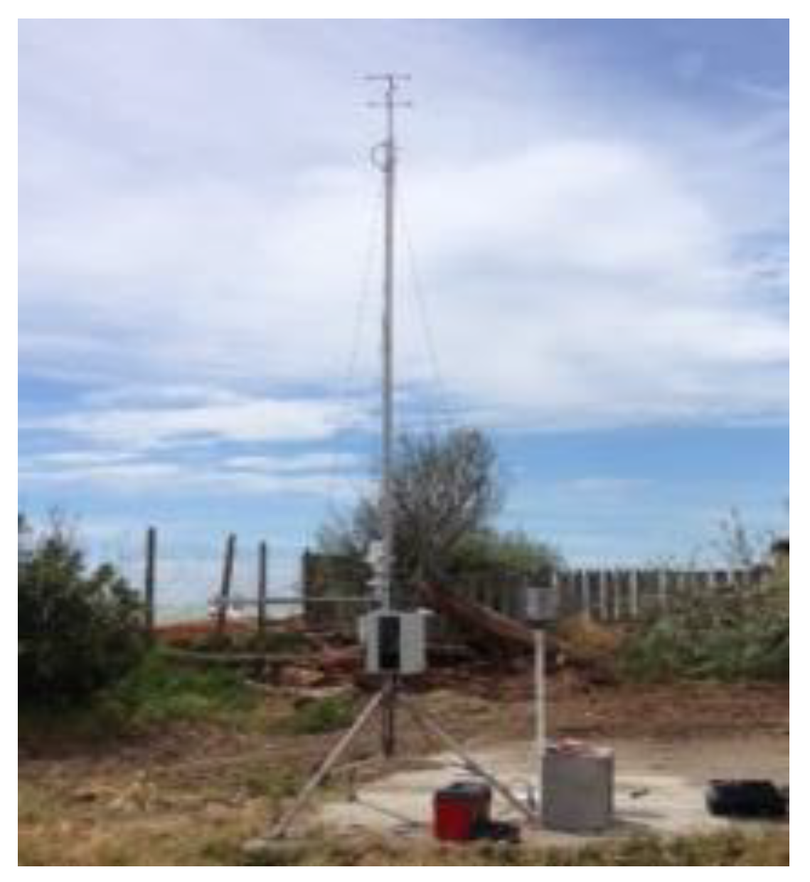
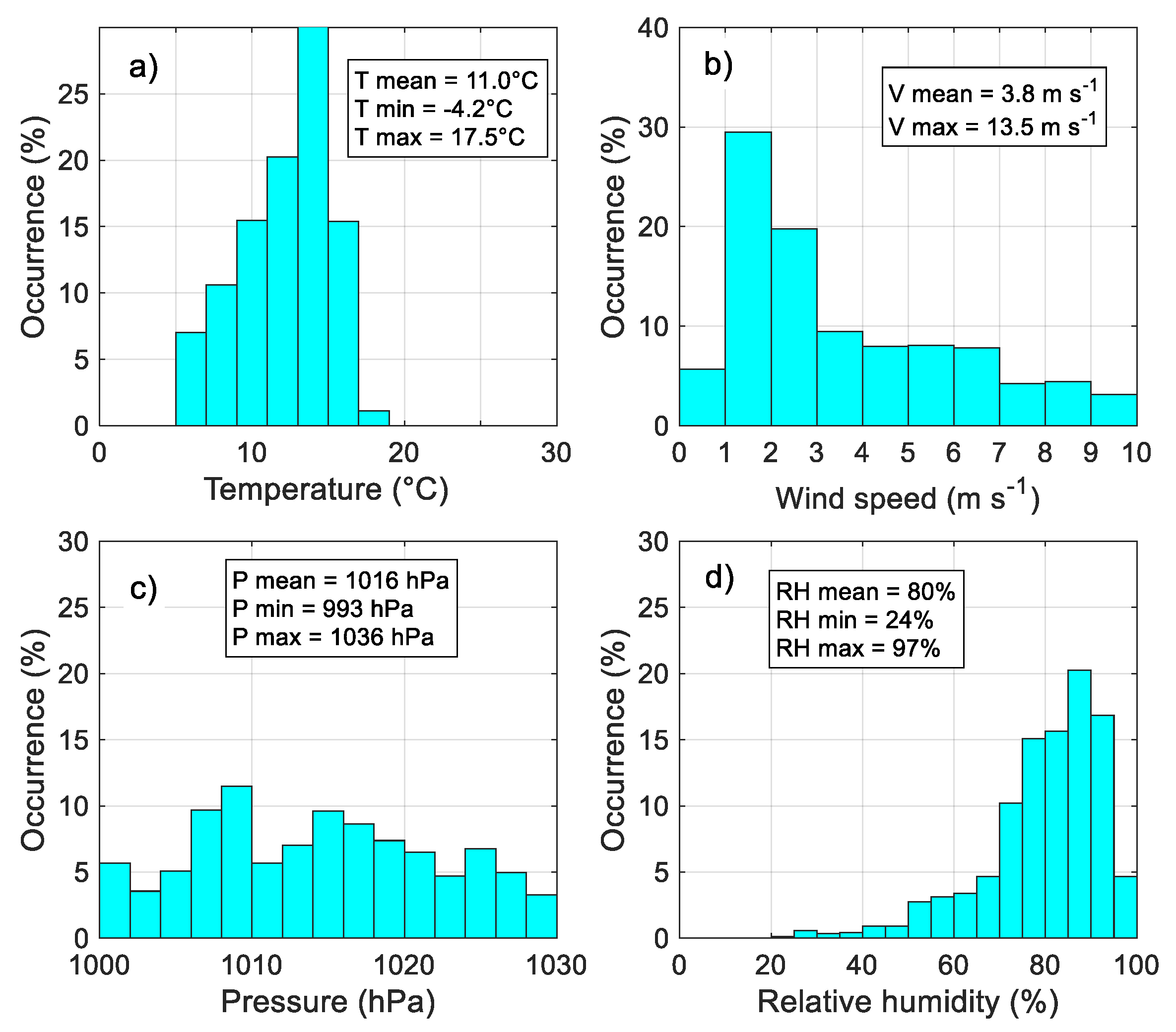
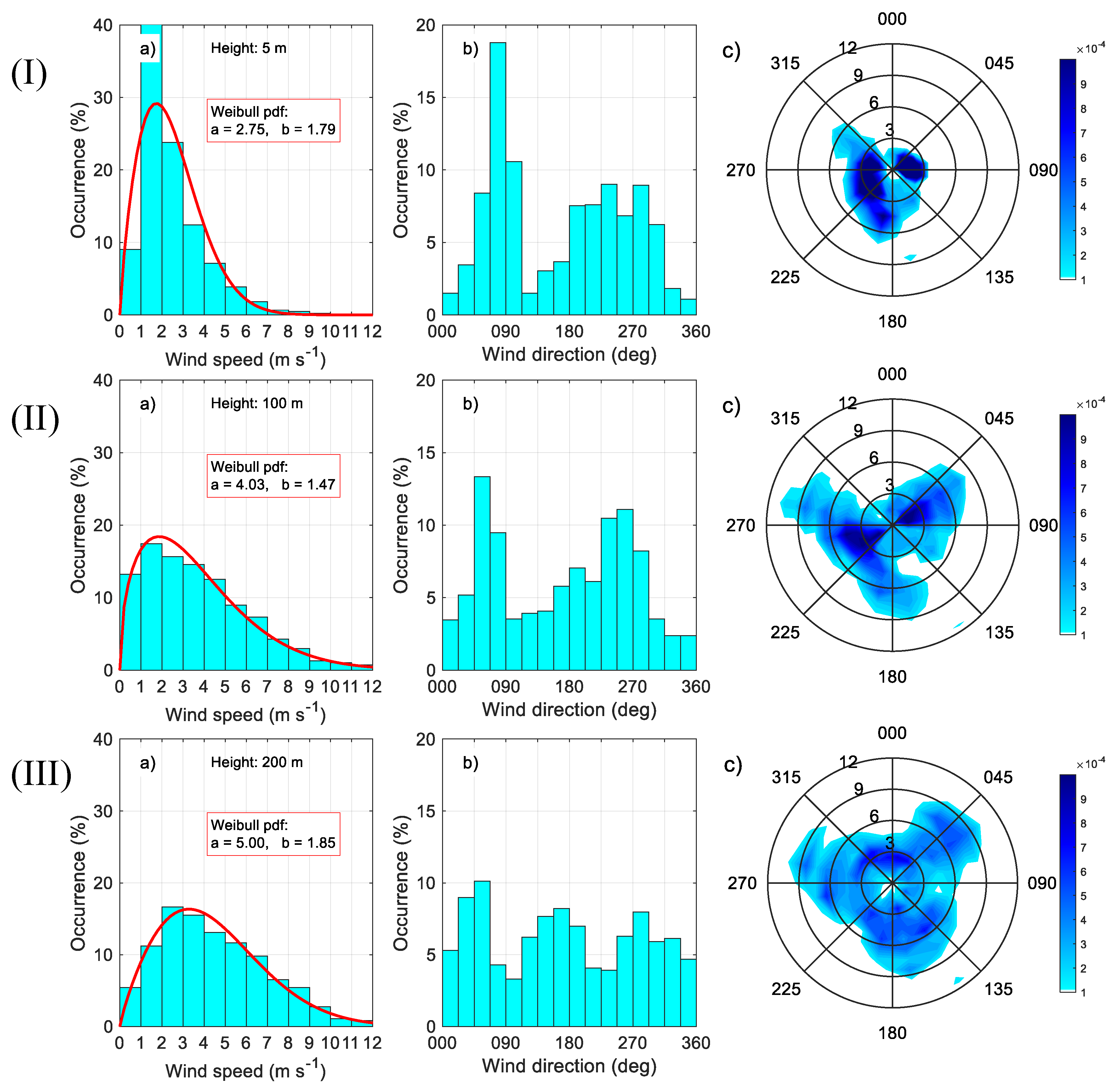
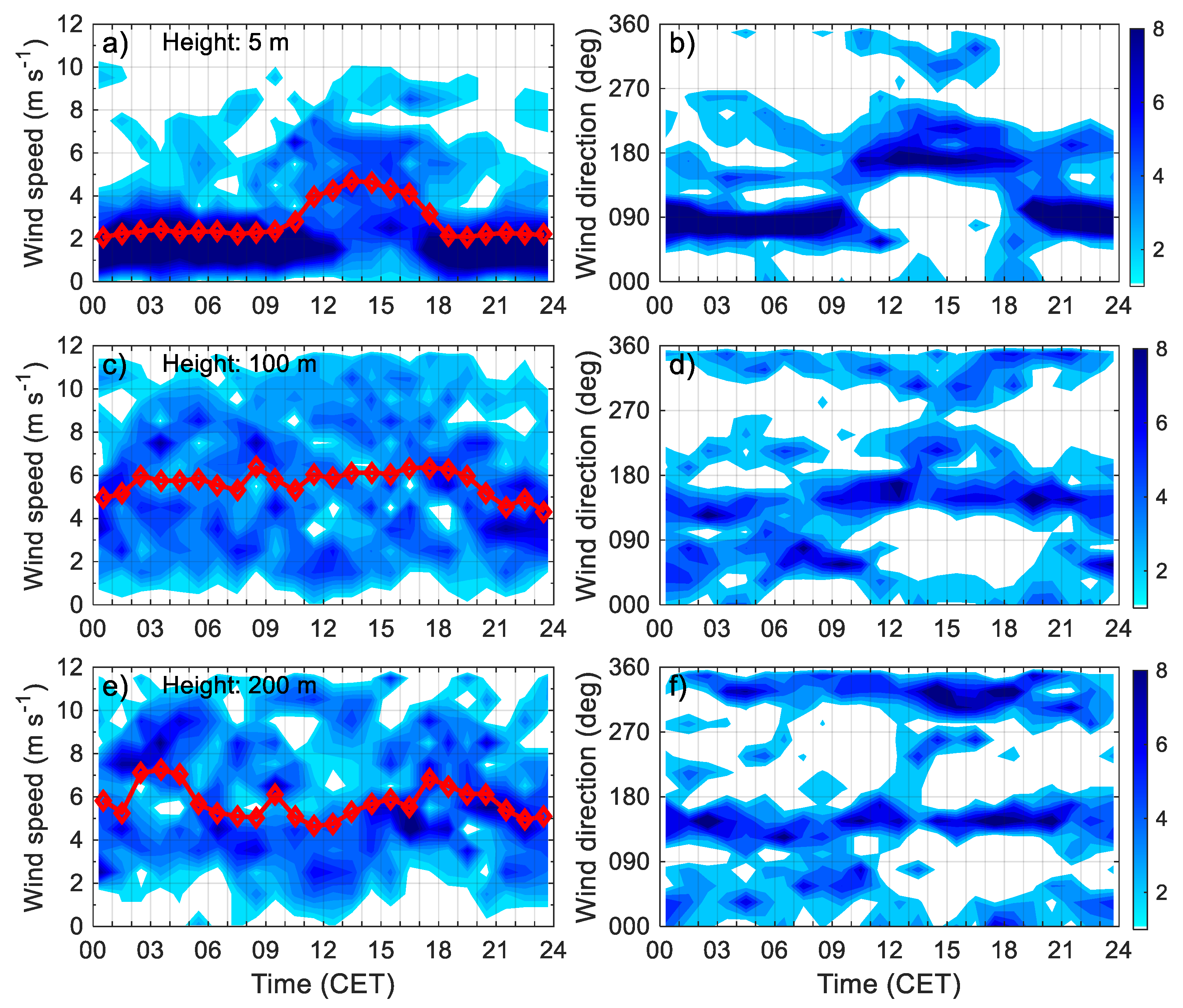
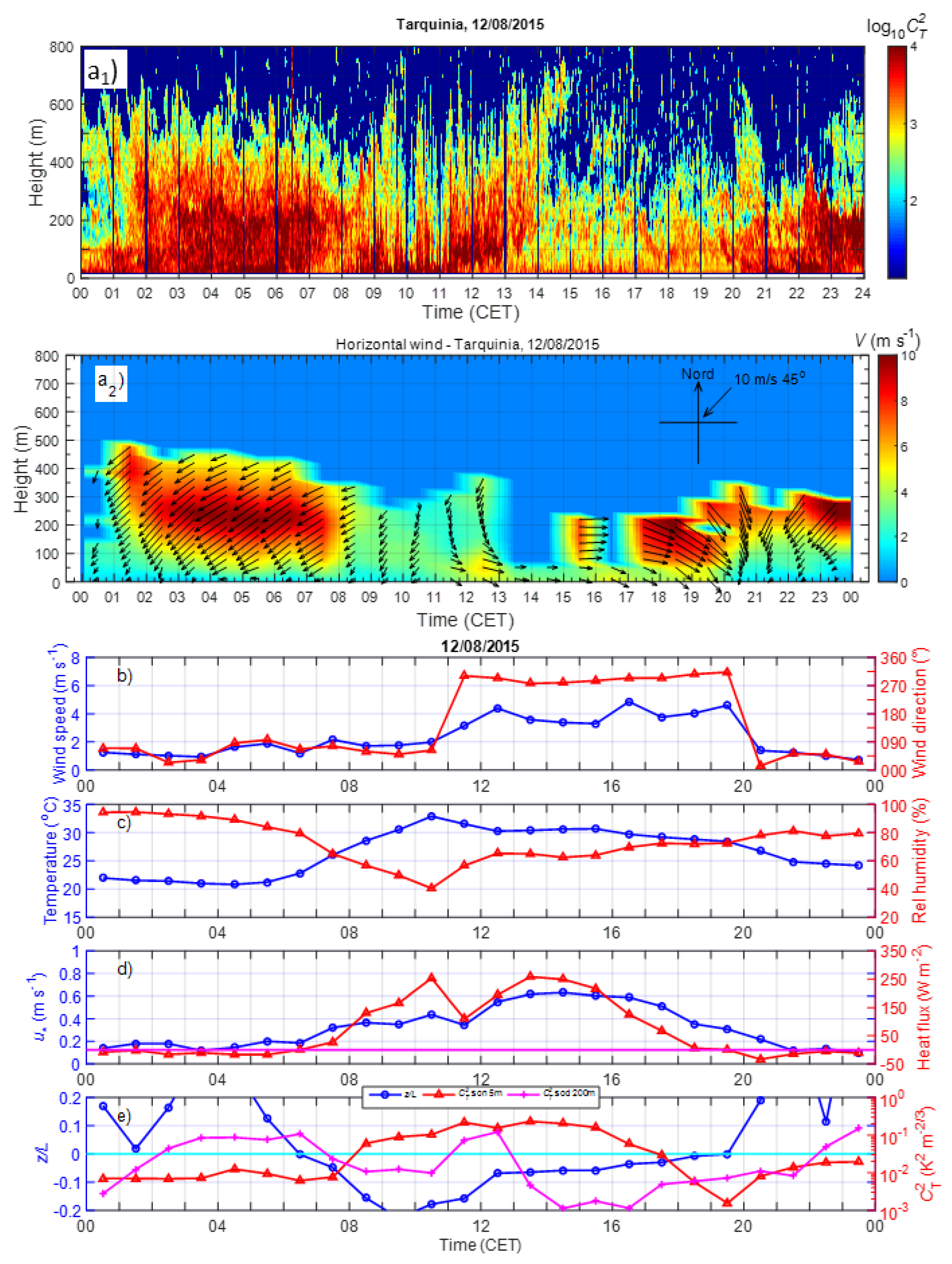
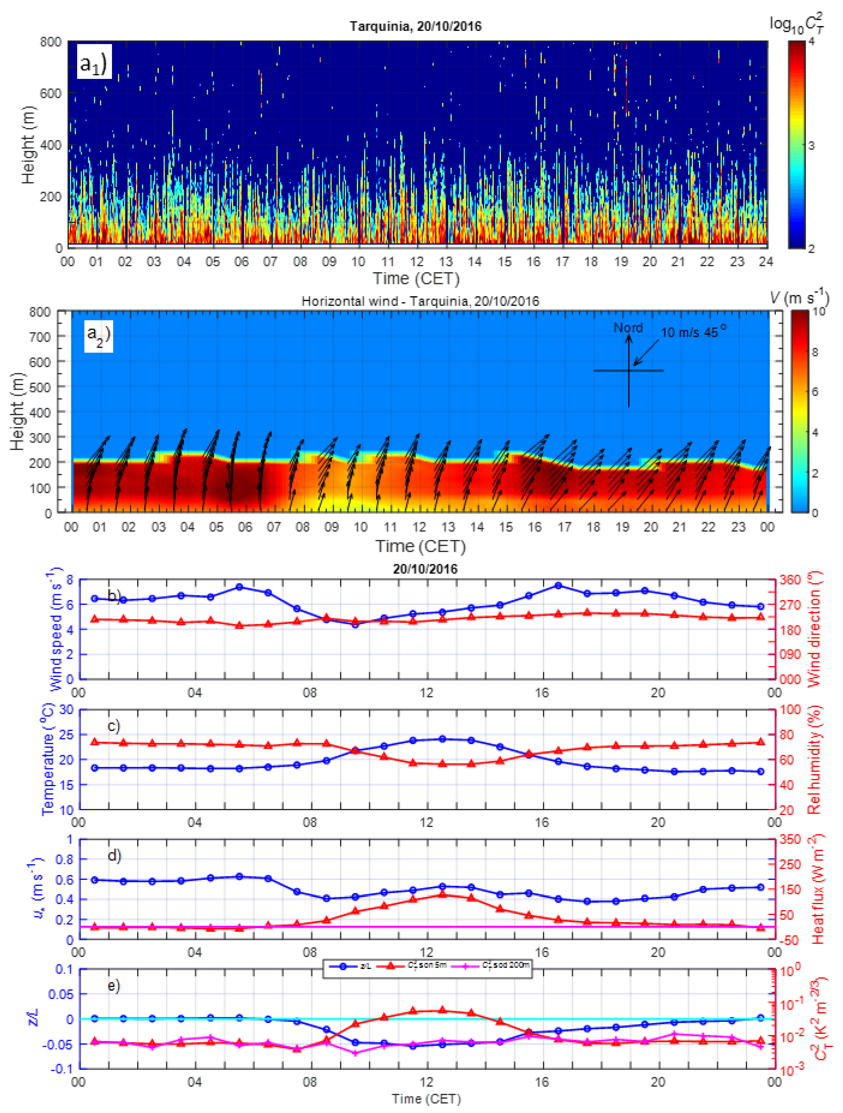
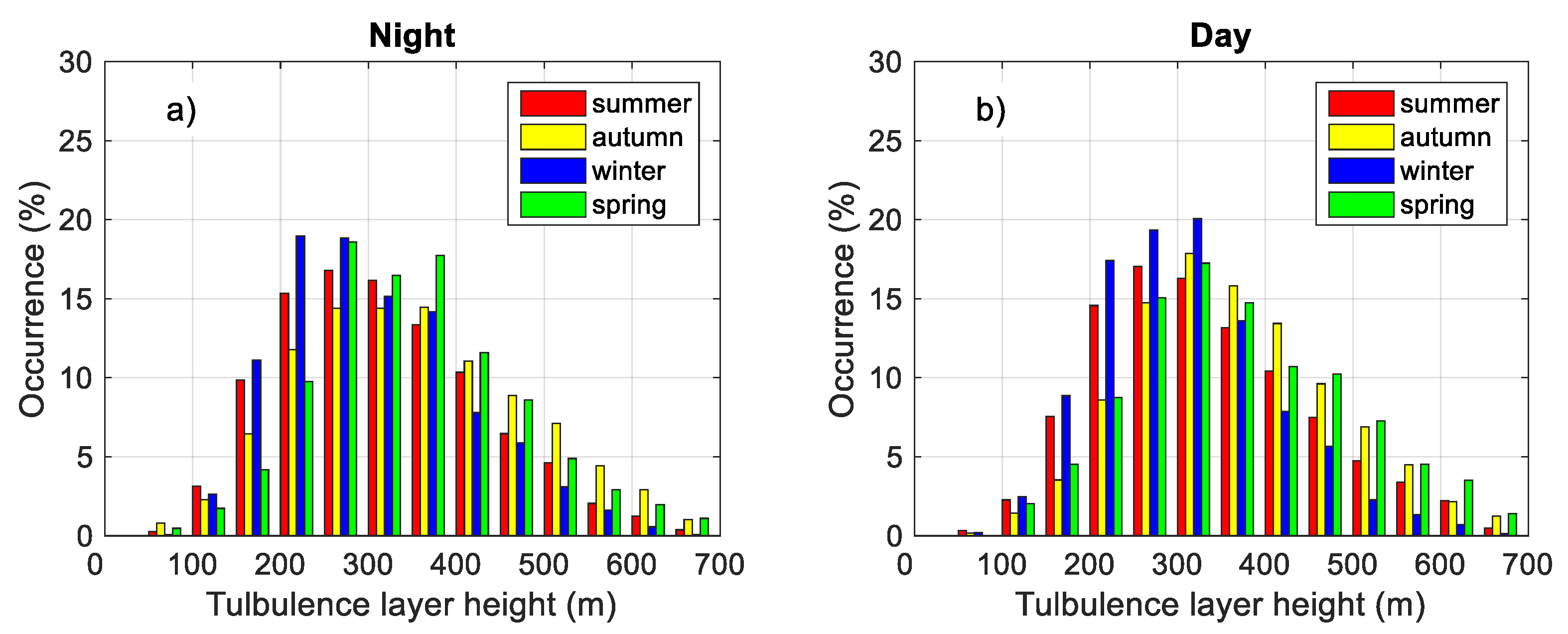
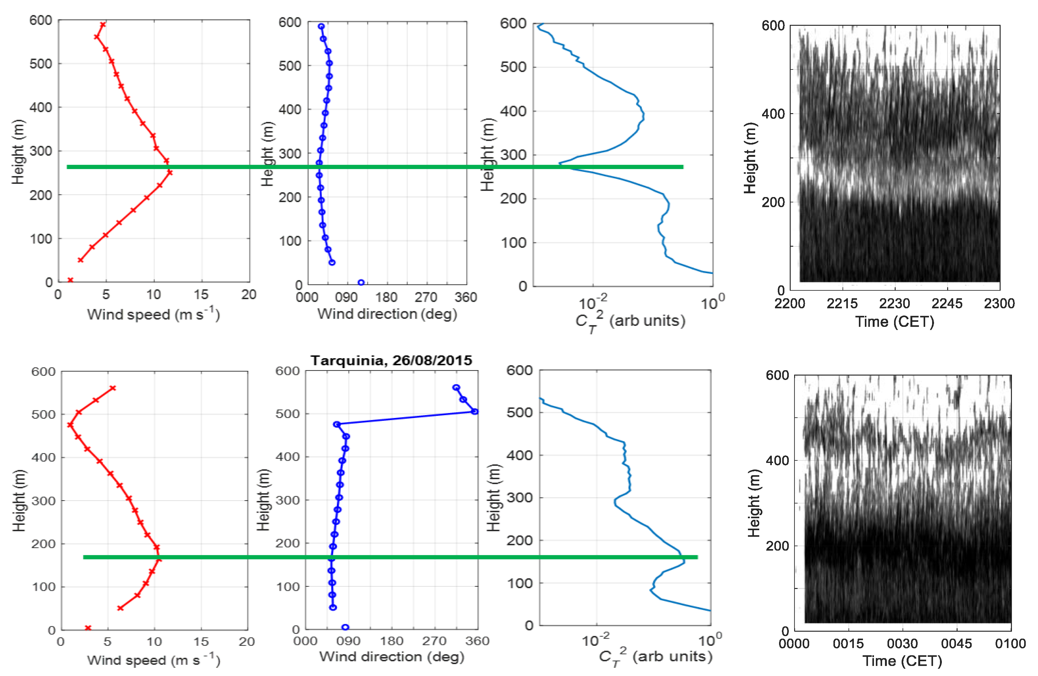
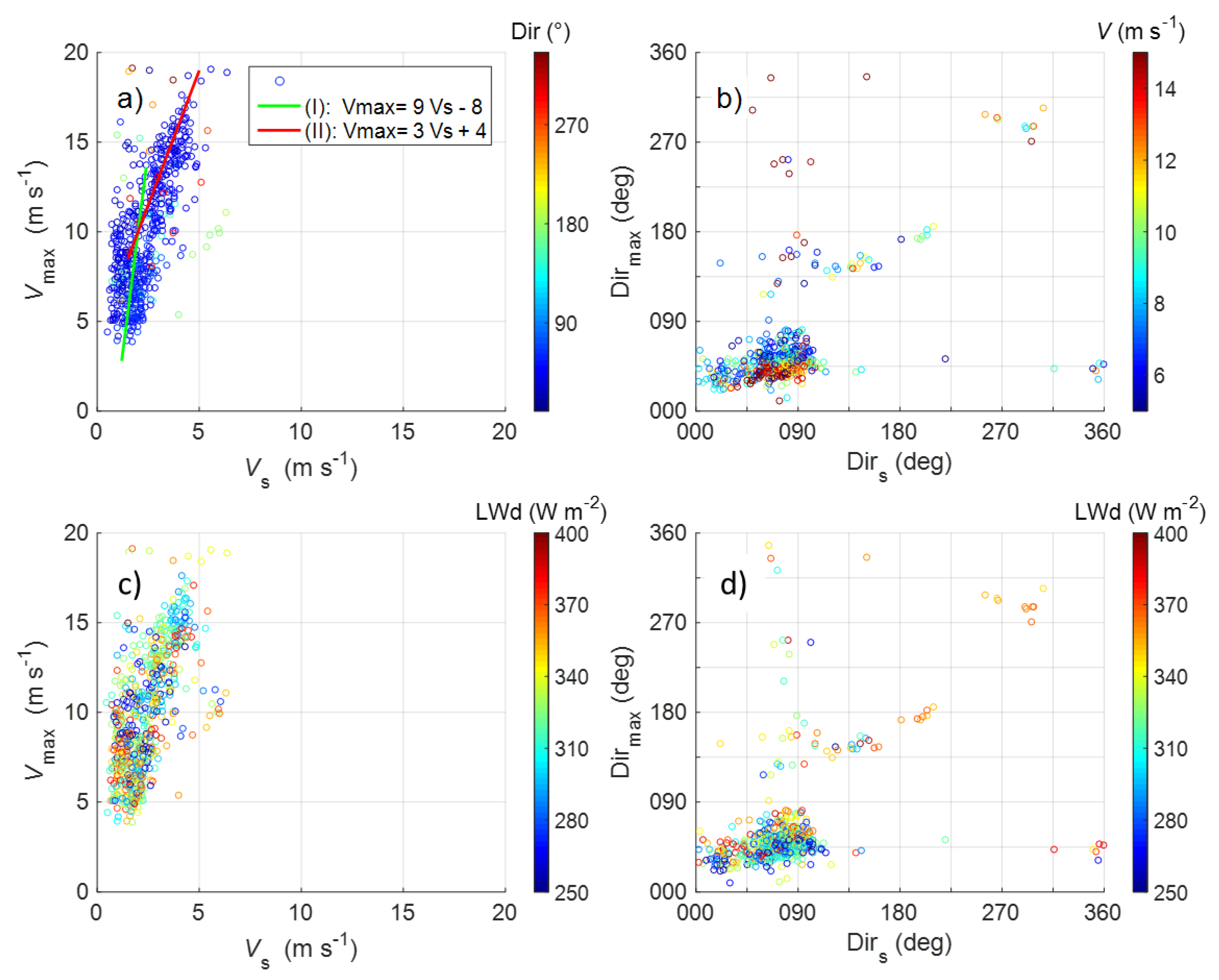
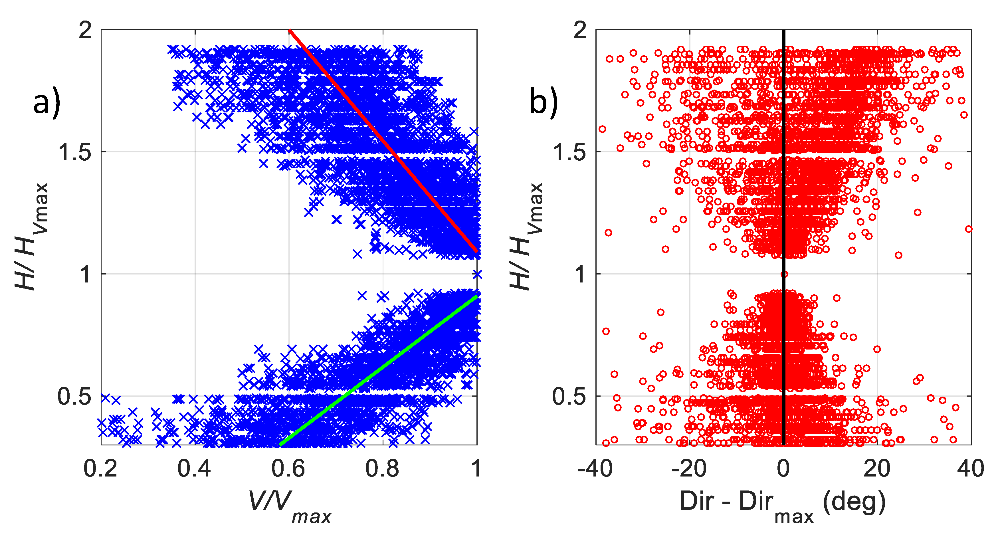
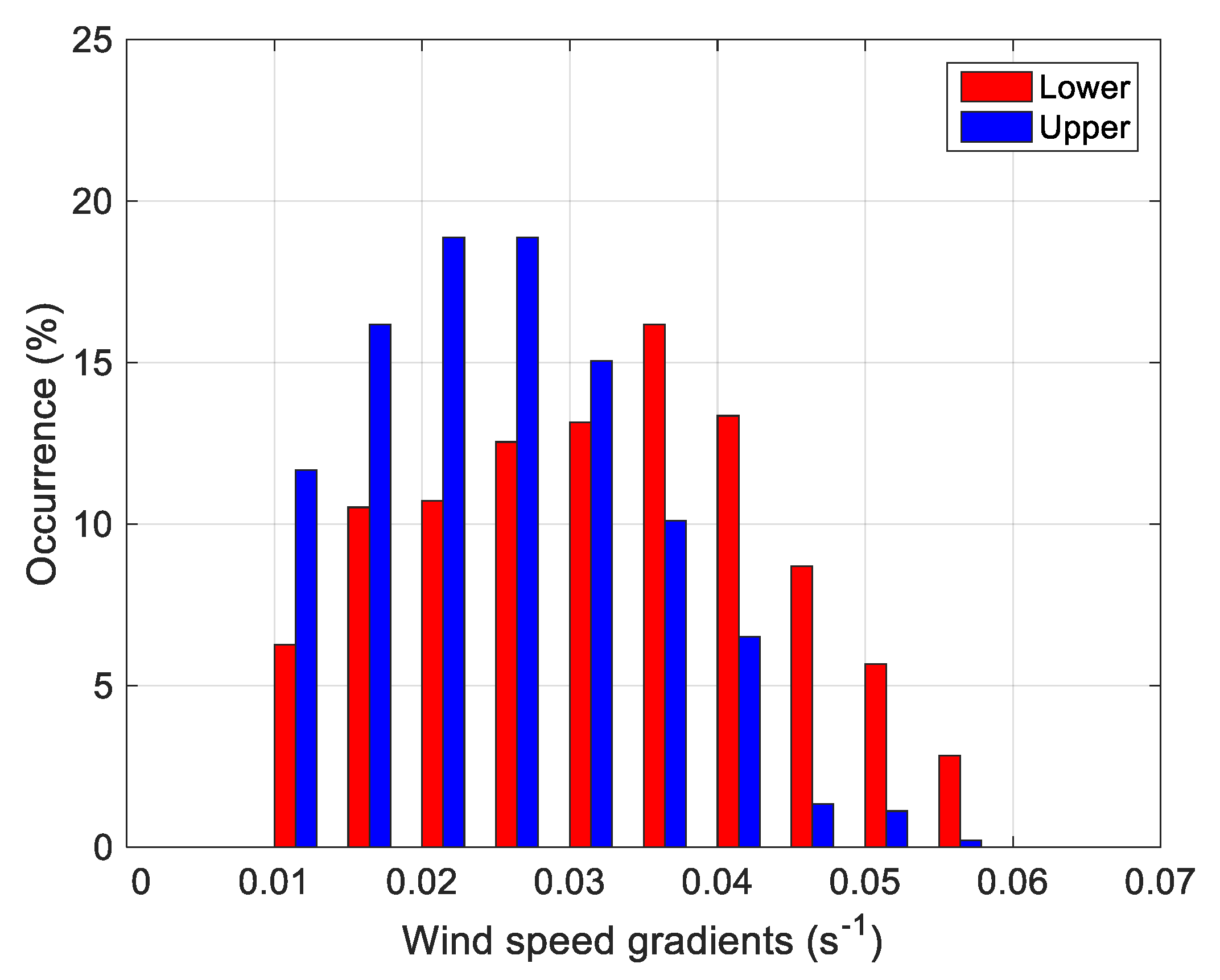
Table 1.
Technical characteristics of the meteorological instruments.
| Instrument | Type | Accuracy | Sampling Period (s) | Heights (m) |
|---|---|---|---|---|
| Ultrasonic anemometer | Metek USA-1 | Wind velocity 0.05 m s−1 Temperature 0.01 °C | 0.1 | 5.2 |
| Thermohygrometer | Vaisala HMP155 | T: 0.15 °C; RH: 1.5% | 60 | 1.8 |
| Net radiometer | Kipp & Zonen CNR1 | Daily sums: 10% | 60 | 1.6 |
| Barometer | Vaisala PTB110 | 0.3 hPa | 60 | 1.0 |
| Rain gage | Lastem C100A | 0.2 mm | 60 | 1.6 |
© 2019 by the authors. Licensee MDPI, Basel, Switzerland. This article is an open access article distributed under the terms and conditions of the Creative Commons Attribution (CC BY) license (http://creativecommons.org/licenses/by/4.0/).
Share and Cite
MDPI and ACS Style
Petenko, I.; Casasanta, G.; Bucci, S.; Kallistratova, M.; Sozzi, R.; Argentini, S. Turbulence, Low-Level Jets, and Waves in the Tyrrhenian Coastal Zone as Shown by Sodar. Atmosphere 2020, 11, 28. https://doi.org/10.3390/atmos11010028
AMA Style
Petenko I, Casasanta G, Bucci S, Kallistratova M, Sozzi R, Argentini S. Turbulence, Low-Level Jets, and Waves in the Tyrrhenian Coastal Zone as Shown by Sodar. Atmosphere. 2020; 11(1):28. https://doi.org/10.3390/atmos11010028
Chicago/Turabian StylePetenko, Igor, Giampietro Casasanta, Simone Bucci, Margarita Kallistratova, Roberto Sozzi, and Stefania Argentini. 2020. "Turbulence, Low-Level Jets, and Waves in the Tyrrhenian Coastal Zone as Shown by Sodar" Atmosphere 11, no. 1: 28. https://doi.org/10.3390/atmos11010028
Note that from the first issue of 2016, this journal uses article numbers instead of page numbers. See further details here.