Radial Distributions of Sea Surface Temperature and Their Impacts on the Rapid Intensification of Typhoon Hato (2017)

Abstract

As a category-3 typhoon, Hato (2017) experienced the notable rapid intensification (RI) over the hot sea surface before its landfall. The RI process and the influences of local sea surface temperature (SST) patterns on the evolution of Hato were well captured and carefully investigated using a high-resolution air–sea coupled model. To further explore the close relationship between the radial distributions of SST and storm evolution, a sensitive experiment with time-fixed SST was also performed. Results showed that the time-fixed SST experiment produced earlier RI following the rapid core structure adjustment, as higher SST in the core region was found favorable to increasing the near-surface water vapor and latent heat flux. Strong updrafts were thus facilitated inside the eyewall, inducing the eyewall contraction and RI of the storm. In contrast, cooler SST inside the core region should account for the delay of RI as the intense convection located in the outer rainbands, inhibiting the transportation of energy into the inner-core. Momentum tendency analysis also proves these mechanisms. Therefore, not only the value of SST but also its radial-gradient, plays an important role in the evolution of tropical cyclones, highlighting the need for an advanced air–sea coupled model.

1. Introduction

Tropical cyclone (TC) is a severe weather phenomenon generating on the warm low-latitude ocean surface that brings much damages and increasing economic losses to the coastal areas every year. Nonetheless, comparing with the increasing capability of the track forecast, the prediction ability for TC intensity has rarely been improved in the recent 30 years [1,2,3,4], especially for the rapidly intensifying TCs over warm oceanic features [5,6,7,8,9,10,11,12]. The main reason is that the rapid intensification (RI) of TCs, defined as an increase of more than 15.4 m s⁻¹ for the maximum 10 m-high wind speed within 24 h [13,14], usually occurs in many intense TCs before attending their peak intensity and produces the largest forecast errors [15,16]. In addition to the lack of ocean in situ observations, pale understandings about the complex ocean feedbacks to the storm structure and evolution also limit the RI forecast development.

Sea surface temperature (SST) distributions under the storm is among the key factors impacting the evolution of TCs [17,18]. In general, high SST benefits the intensification and maintenance of TCs by offering abundant surface moist enthalpy fluxes to the atmosphere. Concurrently, the underlying SST distribution is affected by TCs through oceanic responses to the momentum fluxes and heat exchanges over the air–sea interfaces. Both observations and numerical experiments have shown that the wind-induced vertical diffusions in ocean mixing layer and the upwelling in deeper-layer ocean usually decrease SST, which can thus translate into distinct effects on TCs intensity and structure evolution [6,19,20,21,22,23,24]. Walker et al. [25] observed the maximum SST cooling of 8–9 °C during the slow-moving category-4 Hurricane Kenneth (2005), indicating that both TC intensity and the translation speed play important roles on sea surface cooling. According to the sensitive experiments that conducted by Halliwell et al. [26], small TCs with fast translation speed tend to be less sensitive to the SST changes, owing to the small eyewall coverage of the specific water and insufficient response time. However, Kanada et al. [27] suggested that even weak local SST responses could affect the inner-core structure and intensity evolution in TCs by altering the CAPE and moisture distributions. SST distributions also impact the intensification rate of TCs. By conducting the sensitive experiments with a three-dimensional numerical model, Crnivec et al. [28] concluded that the increasing SST is usually accounting for the increased intensification rate by favoring significant surface moisture flux to the boundary layer. Mean SST higher than 28.5 °C was suggested to be a favorable condition for RI TCs by Kaplan and Demaria [13] comparing with the value of 27.4 °C. Although it has become increasingly clear that there is a strong relationship between SST and RI TCs, the impacts of local SST distributions on the TC inner-core structure and evolution processes are still not well understood.

During the RI processes, in particular at the weak stage of TCs, two specific features are proved to be important: One is the deep updrafts, associated with the high convective available potential energy (CAPE) that transport more low-level moisture to the higher troposphere [24]. With the subsequent release of the principal energy in the upward branch of the secondary circulation, TCs gain the warmer core and increasing intensity. This is known to be the most fundamental process of a TC to transfer heat from the ocean to the atmosphere [29]. With relatively high SST, vigorous diabatic heating induced by the updrafts within the eyewall leads to RI TCs [30,31]. Xu et al. [32] suggested that both size and intensity of a TC were sensitive to the radial distribution of surface entropy flux, indicating the important role of SST distributions under the core region. Another one is the development of asymmetries in the inner-core, which can be an important trigger of the quickly thermodynamic adjustment to the boundary layer. Molinari et al. [33] and Nguyen et al. [34] showed that a TC-like vortex in the inner-core region can spin up from the asymmetric eddies through the wave–mean flow interaction and axisymmetrization process. Both inner-core features are closely related to the SST changes under the eye region. However, how these features response to the local SST changes still need to be illustrated.

TCs that form in the South China Sea (SCS) are usually weaker than those generated in the Northwestern Pacific (NWP) Ocean and have a relatively short time to intensify before they make landfall over south China. Nevertheless, some TCs were reported to experience the RI process and reach the peak intensity before their landfall. Typhoon Vicente (2012) is one of such TCs. Vicente formed over the SCS and underwent extreme RI in northern SCS just before its landfall near the Pearl River Delta region of Guangdong Province [35]. A more recent example is the category-3 Typhoon Hato (2017), which headed west-northwestwards in the northern SCS and also experienced rapid intensification before its landfall. However, the roles that local air–sea interaction play in these TCs is hard to understand because of the insufficient in situ observations. Therefore, developing high-resolution numeric models becomes an urgent need to realize the TCs’ inner-core evolution. Recently, the atmosphere-ocean coupled models promise to be a key forecast tool to simulate TC intensity and structure changes, because the ocean component of these models needs to include the realistic initial conditions to correctly simulate ocean responses to TC forcing [36,37,38], and vise versa. In this study, two numeric simulation are conducted with an atmosphere-ocean coupled model, of which one is with the oceanic responses and the other one is under a fixed SST condition by using the atmospheric component only.

The remainder of this paper is organized as follows. Section 2 introduces the coupled model and the configurations in two experiments. Section 3 details the model results and the causative mechanisms, including the evaluations of the coupled-model simulations and the TC inner-core evolution with different SST distributions. Mechanisms behind the different TC responses are checked based on the latent heat fluxes and azimuthally mean tangential wind tendency. Followed by the discussions in Section 4, the conclusions are given in the fifth section.

2. Data and Methods

2.1. TC Best Track Data and SST Data

The six hurly best-track TC data are obtained from Shanghai Typhoon Institute, China Meteorological Administration (CMA; http://tcdata.typhoon.org.cn), which include the locations of the TC center, central pressure, 10-m maximum sustained wind speed, and the radius of the maximum wind (RMW). The observed daily SST data obtained from the optimally interpolated SST (OI_SST) of Remote Sensing Systems (RSS, http://www.remss.com/measurements/sea-surface-temperature/oisst-description/) with the resolution of 9 km. This product contains observations from TMI, AMSR-E, AMSR2, WindSat, Terra MODDIS, and Aqua MODIS; thus, the complete SST maps can be used to resolve the temperature variability in cloudy situation. After removing the diurnal variation by using a diurnal model, the MV_IR OI_SST represents the SST has been corrected to represent the noon temperature.

2.2. Model and Configurations

In this study, an air–sea coupled model, composed of the advanced research dynamical core of Weather Research and Forecasting model (WRF_ARW, version 3.7 [39]) and the Regional Oceanic Modeling System (ROMS [40]), is used to simulate the ocean responses and feedbacks to the atmosphere. WRF_ARW is a fully compressible, terrain-following vertical coordinate, non-hydrostatical primitive equation atmospheric model with a series of physical schemes to choose. It has been widely used in regional mesoscale atmospheric researches [4,32,34,41,42]. Here, it was configured with 36 vertical levels and the top level at 50 hPa altitude. As is showed in Figure 1, the outmost horizontal domain was set with the resolution of 18 km in size of 231 × 171 grid points, covering an area of Hato (2017) and its environmental fields. Two automatically TC center-following inner domains were downscaled to 6 km and 2 km with domain size of 136 × 124 and 193 × 184 grid points, respectively. During the simulation, two inner domains were adjusted with the TC center every 5 steps. The basic physical options in the WRF_ARW model included the Noah land surface model with Yonsei University planetary boundary layer scheme (YSU_PBL), the Rapid Radiative Transfer Model (RRTM) in computing the long wave radiation, and Dudhia scheme for shortwave radiative effect [43,44]. The SBU-YLin 5-class microphysics scheme from Lin and Colle (2011) was used to resolve the precipitation, featuring water vapor, cloud water, cloud ice, rain, and snow [45]. For the outer 18 km domain, the Kain–Fritsch (KF) scheme [46] was used in Cumulus parameterization. To further improve the simulated TC intensity and trajectory, the grid nudging scheme [47] was applied in the outmost domain every 3 h in all simulations, with a nudging coefficient of 0.0003 s⁻¹ for all horizontal winds, temperature and moisture.

To reproduce the ocean responses to the typhoon forcing, ROMS was coupled to WRF through the Model Coupling Toolkit (MCT). ROMS is a free-surface primitive equation ocean model in sigma vertical coordinate, which has been widely used in estuaries, coastal [48,49], and open ocean simulations [17,50] for both research and operational forecasting (model is developed and supported mainly by researchers at the Rutgers University, University of California Los Angeles, codes available at http://www.myroms.org). Configured with 30 vertical levels and one horizontal domain, the single domain of ROMS covered the same region as WRF did with the horizontal resolution of 18 km, which means that the variables could be transferred from grid to grid between two models. The vertical mixing parameterization scheme was based on the two-equation turbulence model, Generic Length Scale (GLS) parameterization, which is a local closure scheme with the popular k-kl (Mellor-Yamada level 2.5) scheme [51]. During the simulations, the SST from ROMS was passed to WRF_ARW at every five minutes through the coupler. In turn, the surface stresses and net heat flux from the WRF_ARW model were passed to ROMS with 5-mins interval too.

2.3. Experimental Design and Analytical Method

Two experiments were conducted with different SST representations, of which one using the air–sea coupled model (hereafter is named the CPL) and the other one with the WRF model with fixed SST (hereafter is named the FO). In the CPL, the climate condition and initial ocean status in ROMS were from the daily output Hybrid Coordinate Ocean Model (HYCOM) 0.08° operational forecasting data sets, including two-dimensional surface elevation, three-dimensional velocity field, and scalar parameters containing sea temperature and salinity. The ocean topography data, ETOPO1, with the spatial resolution of 1 arc-minute, was obtained from the National Geophysical Data Center (NGDC) (https://www.ngdc.noaa.gov/mgg/global/global.html). For the atmospheric model input, both experiments used the same initial and 3-hours-interval lateral boundary conditions which were downloaded from Global Forecasting System (GFS) datasets with the resolution of 0.25°× 0.25°. The simulations started at 0000 UTC on 22 August and were integrated for 120 h, containing the period from Hato intruded the SCS to 2 days after its landfall. In the CPL simulation, ROMS was forced by the surface stresses and net heat fluxes from WRF model and in return, transferred SST to WRF through the MCT to verify the bottom condition every five minutes. The following atmospheric analyses are based on the hourly outputs while the ocean responses are from the ROMS output with the interval of 3 h.

All parameters in calculating the diagnostic equations are from the WRF outputs. The latent heat flux is calculated based on the bulk formula.

$$LHF=\rho L_v{C}_q{U}_a\mathsf{\Delta }q$$

(1)

where $\mathsf{\Delta }q=\left(q_s-q_a\right)$, q${}_s$ is the surface saturation, and q${}_a$ denotes the mixing ratio of the water vapor on the lowest model level. U${}_a$ is the horizontal wind speed at the same altitude with q${}_a$. $\rho$ is the air density in surface layer; L${}_v$ denotes the latent heat of vaporization; C${}_q$ is the surface exchange coefficients for moisture.

The azimuthally mean tangential wind tendency equation reads

$$\frac{\partial \overline{v}}{\partial t}=-\overline{u}{\overline{\zeta }}_a-\overline{w}\frac{\partial \overline{v}}{\partial z}-\overline{u^{\prime }{\zeta }_a^{\prime }}-\overline{w^{\prime }\left(\frac{\partial v^{\prime }}{\partial z}\right)}+{\overline{F}}_{fric}+{\overline{F}}_{diff}$$

(2)

where u, v, and w denote the storm-relative radial, tangential, and vertical winds, respectively. ${\zeta }_a=\partial v/\partial r+v/r+f$, is absolute vorticity. The over bars denote the azimuthal average and primes are the deviation from averaged values. The lhs of Equation (2) is the azimuthally averaged tangential wind tendency. First four terms on the rhs of Equation (2) are the mean radial flux of absolute vertical vorticity (RADV), the vertical advection of azimuthal mean tangential wind by the mean updrafts (VADV), the radial eddy flux of perturbation vorticity (REDY), and the vertical advection of asymmetric tangential wind through the asymmetric portion of updrafts (VEDY). The last two terms are the turbulent vertical mixing including surface friction in the boundary layer and the sub-grid horizontal diffusion, respectively. Due to the small magnitude (<1%), the term VEDY could be neglected.

For further analysis, the potential vorticity (PV) and eddy kinetic energy (EKE) is also calculated. PV writes as

$$\mathrm{PV}=-\mathrm{g}{\zeta }_a\frac{\partial \mathsf{\Theta }}{\partial \mathrm{p}}$$

(3)

where the $\mathrm{g}$, $\mathsf{\Theta }$ and $\mathrm{p}$ are the gravitational acceleration, potential temperature and the pressure, respectively. ${\zeta }_a$ is absolute vorticity, same with the definition in Equation (2). The EKE writes as follows

$$\mathrm{EKE}=\left(u^{\prime 2}+v^{\prime 2}\right)/2$$

(4)

where $u^{\prime }$ and $v^{\prime }$ were asymmetric tangential and radial wind velocity, respectively.

3. Results

3.1. Typhoon Hato with SST Distributions

Typhoon Hato (2017) had a northwesterly path in northern SCS, passing across the Luzon Strait at about 0000 UTC on 22 August with the maximum wind speed ~25 m s⁻¹ and minimum sea-surface level pressure (MSLP) of 985 hPa (Figure 2) according to the “best track” data. In the following 18 h, Hato strengthened to ~38 m s⁻¹ with a translation speed of ~8.0 m s⁻¹, though the maximum intensity showed a short-time stagnant near 1500 UTC 22 August. Subsequently, Hato upgraded to category-2 typhoon with the maximum wind speed of 42 m s⁻¹ and a central pressure of 966 hPa just before the midnight of 22 and into 23 August. Hato made its landfall near Zhuhai, Guangdong Province (113.2° E, 22.1° N) at 0450 UTC on 23 August with the 10-m wind speed reached to 51.7 m s⁻¹ and the central pressure of 948 hPa. Soon after its landfall, Hato weakened quickly to 30 m s⁻¹ in several hours and dissipated by 0800 UTC on 24 August.

In both simulations, the northwesterly tracks of Typhoon Hato are qualitatively close to the best track data over the SCS, except for a slight southward shift from 1200 UTC to 2100 UTC 22 August (Figure 2). Given the first 9-hour spin-up period, the intensity of simulated storms in both experiments are similar by the 12-h simulation, but then the FO storm starts to intensify quickly whereas the CPL one experiences a short-time weakening around 1500 UTC on 22 August. Hato does not regain the rapid intensification status until 1800 UTC in the CPL, which is almost 3 h later than the FO storm. By the time Hato makes its landfall, the maximum 10-m high wind speed (VMAX) in the FO experiment is about 5 m s⁻¹ stronger than the best track data and is 6.5 m s⁻¹ higher than the CPL storm. Therefore, the CPL experiment outputs more accurate intensity and track of Typhoon Hato though the minimum sea level pressure is relatively higher than the observations. In this study, as the intensification time for Hato is less than 24 h, RI is defined as the time when VMAX exceeded 36.0 m s⁻¹ and the VMAX should increase in the first 6 h.

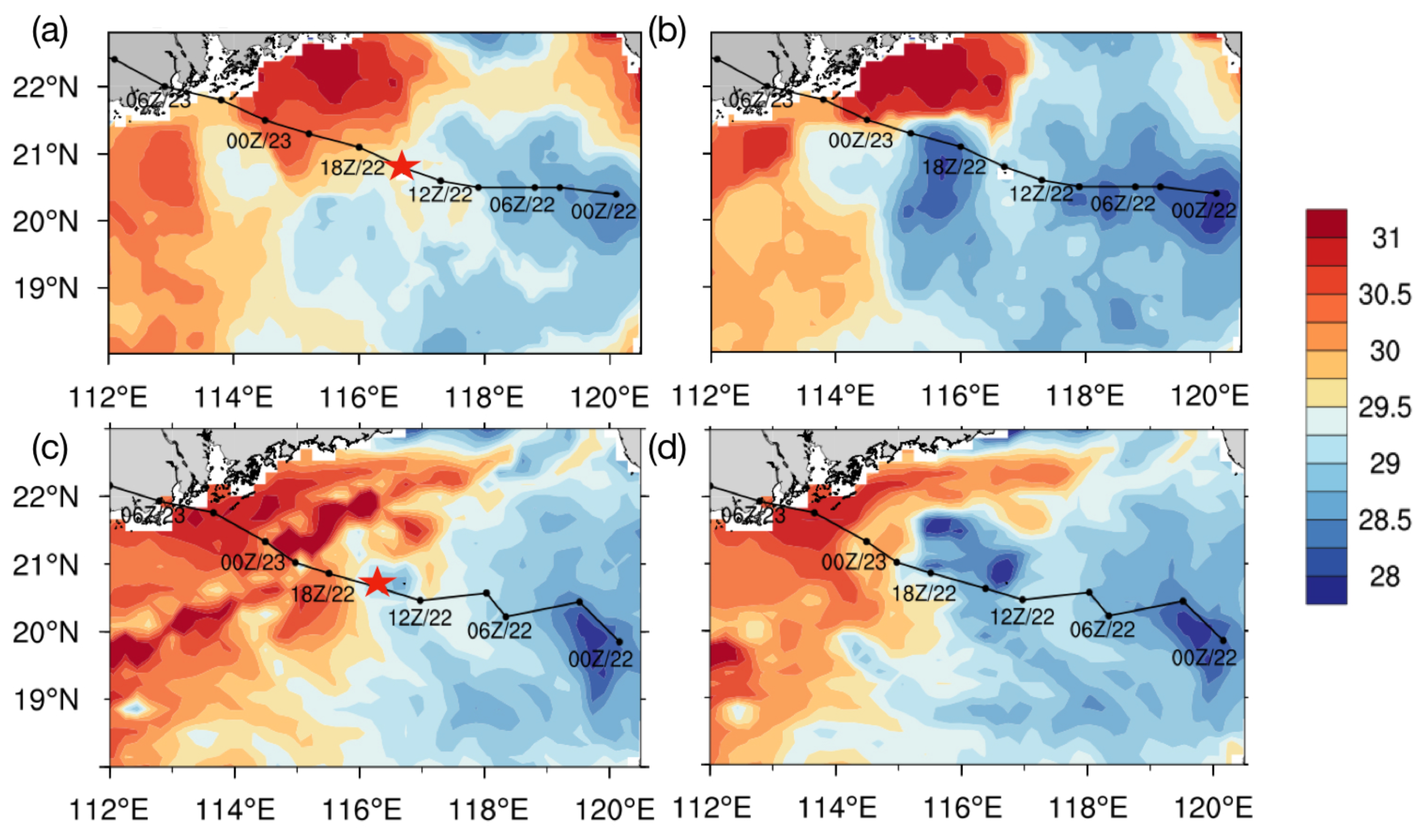
As is shown in Figure 3a, the SST over northern SCS is broadly higher than 28.5 °C by the noontime on 22 August, supplying adequate heat for the rapid intensification of Hato. Over the shallow continental shelf inhabits a thin warm layer with the surface temperature higher than 30.5 °C, whereas the simulated SST is 0.5 °C cooler than the satellite SST. At 1200 UTC 23 August, the satellites observed SST (Figure 3b) cools down by 0.5–1.5 °C beneath the track of Hato but warm SST remained higher than 30 °C near the coastline. The CPL simulated SST pattern at 1200 UTC August 22 is generally consistent with the satellite observations (Figure 3c) with more uniform distribution on the continental shelf and relatively warmer SST over the open sea. One exceptionally cool region, where the SST drops down to ~28.2 °C to the northwest of the Luzon island, is possibly due to the strong simulated vertical mixing over an annually upwelling zone according to the study of Hu et al. [52]. By 1200 UTC on 23 August, the CPL SST captures the surface cooling in the open SCS and the warm layer in the neritic except for a cooling zone over the shelf break which slightly shifts to the north of the track.

The simulated surface cooling during the passage of Hato through the northern SCS, defined as the SST change from the initial time to 30 h throughout the simulation, is depicted in Figure 4a. The major cooling, peaking at approximately −1.7 °C, appears to the rhs of the track from around 117.0° E longitude to the edge of continental shelf and is roughly parallel to the shelf break. Such right-hand-side cooling is usually associated with a strong and fast-moving typhoon, as was suggested in earlier studies [8,27,36]. SST over the shallow continental shelf barely cooled, which is also similar to the observations. Figure 4b shows the hourly local averaged SST changes of the core-region (within 60 km radius) in both experiments. The local averaged SST in FO experiment presents an increasing trend with time and higher value than the CPL results, especially during the period of from 1200 UTC to 1700 UTC 22 August, whereas CPL SST is steady or even lower than the initial value. Concurrently, the FO storm starts RI while the CPL storm intensity is slightly weakened (Figure 2a) owing to the cooling SST band under the core region.

Detailed SST distributions associating with the simulated storms at 1400 UTC and 2100 UTC 22 August are depicted in Figure 5. By 1400 UTC 22 August, a narrow cold SST band appears under the storm inner core with the minimum value of 28.7 °C (Figure 5a). This cooling band strengthens to lower than 28.6 °C during the next 7 h and keeps impacting the CPL storm until 2100 UTC 22 August, when the inner-core of Hato moves out of the cooling area with large northwesterly translation speed of ~8.0 m s⁻¹ (Figure 5c). In contrast, the time-fixed SST in FO experiment is ~0.8 °C higher than that in the CPL one and the original cool band is much weaker to the right of the eye region. The CPL simulated SST becomes ~0.4 cooler than the fixed SST over the broad sea surface (Figure 5c,f) except for the coastal areas, where similar phenomenons were also reported by Miles et al. [48] and Zhang et al. [36]. Another notable feature is that the FO storm also appears a distinctive asymmetric core structure at 1400 UTC 22 August, as was shown by the scrambled wind vector within the 980 hPa isoline (Figure 5b). This would be analyzed in the following text. Note that the eye of a TC, defined as the location with MSLP within 200 km radius, could be quite near to the maximum wind, especially during the early weak stage.

3.2. Storm Structures Associated with Local SST Patterns

The snapshots of composite reflectivity ranging from 1400 UTC to 1700 UTC 22 August in both experiments are shown in Figure 6. Convective activities in CPL storm are weaker than the FO TC, as is referred by the smaller values in both spiral rainbands and inner-core region. Some high reflectivity clusters only appear in the front-left of CPL storm eyewall, where locates higher SST than the inner-core region. In the following hours, deep and strong convections that are far from the primary eyewall move towards the inner-core region. By 1700 UTC 22 August, the outer convective clusters of CPL storm merge into the primary eyewall, leading to larger reflectivity in the eyewall and a more compact structure. Contrastively, the convection in the FO storm is more active over the uniformly warm ocean surface and is in the period of RI (Figure 2a). Though an evident asymmetric structure could be seen in the storm inner-core during the early stage, it quickly adjusts to a rounded eye with stronger rainbands. This suggests that the local SST pattern could largely impact the active convection over it and, thus the core structure of TC.

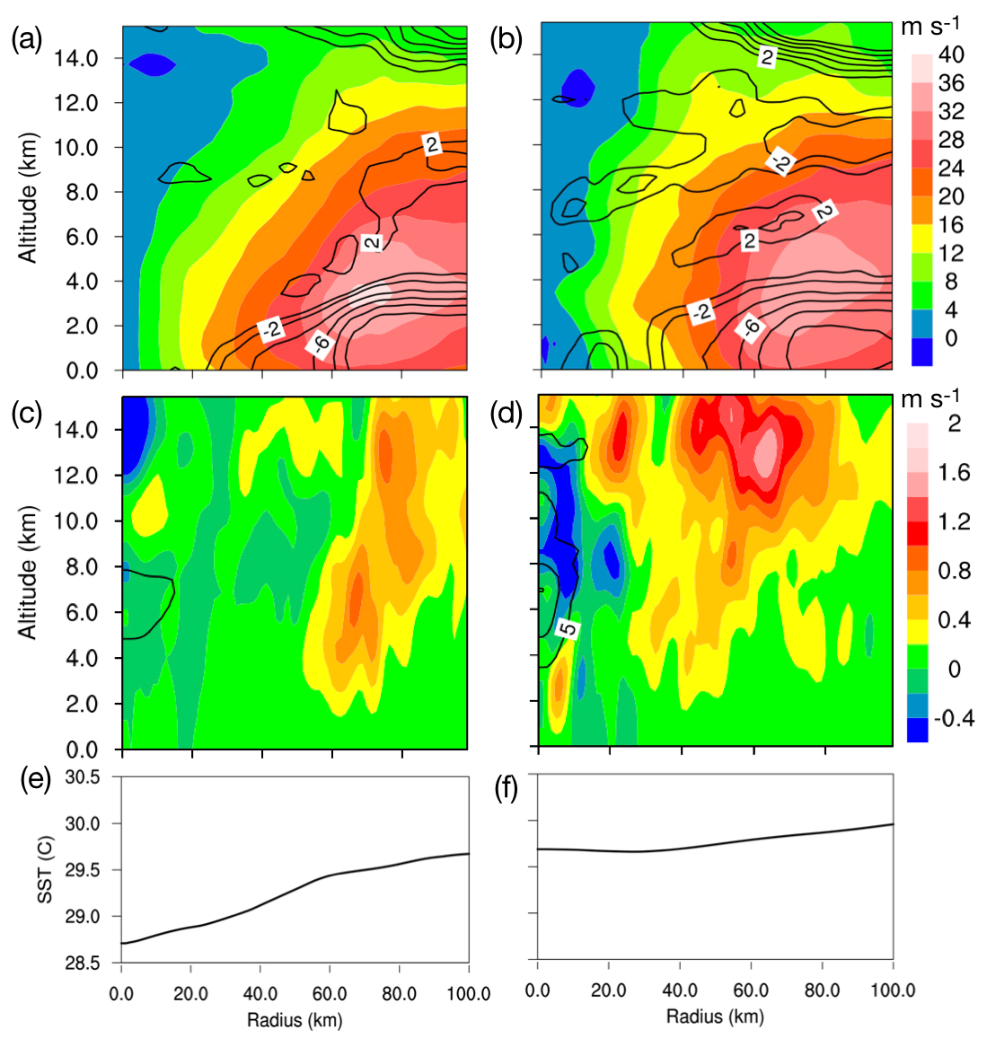
The vertical storm inner core structures vary greatly under different radial SST distributions. Figure 7 shows the azimuthally averaged atmospheric parameters and SST at 1400 UTC on 22 August, when evident SST cooling appears under the CPL storm. Hereinafter, the inner core size is defined roughly as the radius of VMAX (RMW). After 14-h simulation, the azimuthal mean SST in the core region decreases with the appearance of the cooling band. The minimum value is ~28.7 °C and gradually increases outwards to 29.7 °C at 100 km radius. The tangential wind speed is still low within 40 km radius and eyewall tilts outwards, indicating the low heating efficiency in the storm core region. Therefore, the potential temperature anomaly centers at the middle level (~7 km) with the peaking value of about 5 °C. Two branches of intense updraft center outer of the core region of CPL storm at 60–80 km radii, where SST being above ~29.5 °C. Notable inflows could be seen under the primary circulation, indicating the quick eye contraction.

The azimuthally averaged SST below FO storm, however, is uniformly warm at ~29.7 °C, which is ~1.0 °C higher than the core region in CPL storm. In contrast with the weak and loose updraft in CPL storm, intense updraft can be seen at almost all radii behind a 10 km radius (Figure 7b), especially on high altitude (around 12.5 km) with the maximum value of 1.4 m s⁻¹. The mean tangential wind fields develop higher than CPL storm, though the maximum wind speed is slightly weaker. This should be partly ascribed to the asymmetric inner core in the early stage. A vimineous warm core is evident in the middle-to-high level, peaking at 10 °C. Based on the earlier work [53], strong updrafts, high-level outflows, and significant warm core over the warm water are necessities to the storm RI and RMW quickly contraction. With all these conditions, the FO storm undergoes RI earlier than the CPL storm.

By 1700 UTC 22 August, the SST gradient under CPL storm inner-core decreases and the minimum value elevates to ~29.6 °C (Figure 8a). Combine with the increasing low-level inflows, the two branches of updrafts move ~20 km towards the eye and merge at the radius of 60–80 km, peaking at the value of 1.6 m s⁻¹ on 13 km altitude. Due to the strengthened updrafts and mid-to-higher level outflows, the mean tangential wind develops higher and the eyewall tilt less than 1400 UTC. Both intensified updrafts and inflow indicate the onset of RI in CPL storm.

In contrast, the FO storm is undoubtedly stronger than the CPL storm, including the enlarged warm-core, compact eye and less tilt eyewall (Figure 8b,d). Although the local SST under FO storm is just 0.3 °C higher than CPL storm, the updrafts generate broadly from 40 km radius with several centers aligning vertically in the eyewall. The maximum value appears higher and 0.4 m s⁻¹ stronger than the CPL storm.

During the following experimental period, both simulated storms approach the warmer coastal sea surface and undergo RI with increasing updrafts and evident warm-core. The FO storm is still stronger than the CPL one (not shown). Such an intensification process maintains even under the friction effects of the land. Therefore, local SST distributions, as the determining factor of the energy source for TCs, present a strong correlation with the generation of eyewall circulations and thus the storm structure characters.

3.3. Storm Inner-Core Evolution with Local SST Changes

The hourly evolution of the azimuthally averaged tangential wind and radial inflows on the lowest model level (about 30.3 m altitude) are detailed from 0600 UTC 22 August to 0300 UTC 23 August (also shown as the 27 h in the simulation) in Figure 9. Despite the RMW, the radius of azimuthally averaged damaging wind (RDW) is defined as the scope where wind speed excesses 25.7 m s⁻¹. These two indices are proved to be good indications of the storm size evolution based on the discussions in Xu and Wang [32].

Both azimuthally averaged tangential and radial wind of the CPL storm are stronger than the FO storm in the early stage. This is partly because of the highly asymmetric structure of the FO core, as is showed by the shifting RMW. On the other hands, the SST of the two experiments didn’t differ much, which impacts the storm equally. As the SST under the CPL storm inner-core continued to decrease, the tangential wind was suppressed. Therefore, the core develops slowly, showing less compact than that of FO storm with an RMW of ~60 km. In contrast, the FO storm underwent the onset of RI after a quick eye contraction near 1200 UTC 22 August and presented a steady RMW and enlarged RDW. It was not until 1700 UTC 22 August that the CPL storm started its RI with moderate eye contraction, when the core region got rid of the cooling SST band. RDW also expands moderately to ~90 km, indicating the slow development of the prime circulation with warming SST in the late stage.

To examine the effects of local SST changes on the evolution of mid-to-higher level updrafts, the radial-time averaged updrafts at 6.5 km and 12 km altitude are plotted in Figure 10. For both experiments, the eyewall updrafts in the upper-tropospheric (Figure 10c,d) present more sensitivity to the SST distributions than the mid-layer, as is referred to by the larger magnitude of the value and significant changes. Consistent with the similar initial SST patterns, the vertical velocity is weak and differs little in both simulations until 1200 UTC 22 August. Then, local SST patterns differ greatly along with effective ocean responses. For the CPL storm, SST under the eye region shows an evident cooling core between 1300 UTC and 1700 UTC on 22 August. Intense updraft thus only occurred out of 70 km radius, where SST is above ~29.5 °C (Figure 10a,c). After 1800 UTC 22 August, Hato moves out of the cooling band and updraft intensifies quickly near the 75 km radius. The radial SST is uniformly warm with a value of 29.5 °C. Subsequent mid-level updrafts in the CPL storm develop at ∼70 km radius and moves slightly inwards, associating with the gradually increasing SST. Throughout the rest of the simulation, 12-km altitude updrafts are aligned at the ~70 km radius, reaching a value above 2 m s⁻¹.

Eyewall updrafts in the FO storm, however, intensified broadly from 20 km to 80 km radius with a asymmetric core structure, peaking at ~1.75 m s⁻¹, where SST is ~29.7 °C (Figure 10b,d). Significant updrafts maintained on the 12 km altitude, leading to asymmetrical RI process of FO storm. These results suggest that the eyewall updrafts, the leading factor of storm intensification, can be largely impacted by different radial SST distributions especially at the early stage of RI.

The axisymmetricity is usually another important parameter in a RI typhoon, which indicates the degree of axisymmetry for a TC vortex [54,55]. Fudeyasu et al. [54] defined the axisymmetricity as the ratio of the azimuthal mean kinetic energy to the total kinetic energy within a radius of 301 km. Here, we follow this definition using kinetic energy but instead of the area-averaged axisymmetricity used in Fudeyasu et al. [54], we calculate the axisymmetricity for each radial band of 1.25 km to examine the time evolution of axisymmetricity as a function of radius. Figure 11 shows the time evolution of the axisymmetricity in the simulated storms as a function of the radius at 6.5 km and 12.0 km altitude.

Consistent with the above analysis, the FO storm is more asymmetrical before 1200 UTC 22 August. The axisymmetrization occurs significantly on 12 km altitude with the axisymmetricity parameter raising to 0.75 quickly after 1400 UTC 22 August (Figure 11d). The subsequent axisymmetrization is evident near the eyewall between 50 and 90 km, peaking at the value of 0.95. Associating with the strong axisymmetricity, the outer-core sizes of FO storm enlarge considerably. As suggested in the earlier work of Wang and Wang [42], the axisymmetrization always follows the merging of a low-level synoptic depression into the typhoon vortex, which is a critical role in triggering/enhancing the active spiral rainbands in a storm. They also proved that the diabatic heating in spiral rainbands could drive centripetal radial winds in the mid-to-lower troposphere, leading to the acceleration of tangential winds outside the RMW and the significant outward expansion of the storm inner-core size.

The CPL storm gained a more axisymmetric structure on the middle-to-low level than the FO storm before the cooling SST band appeared. However, then it turns to be less axisymmetry at all radii until 1800 UTC 22 August (Figure 11a). Evident axisymmetrization then started from the mid-to-lower troposphere upward after the onset of RI. By 2100 UTC 22 August, the mid-level maximum axisymmetricity parameter (close to 0.93) appears near the outer edge of the eyewall where SST increases relatively high (above 29.8 °C). The storm becomes more axisymmetric at larger radii during the following hours. However, the axisymmetricity parameter on the 12 km altitude becomes much smaller after 1800 UTC, indicating a less favorable high-level condition. The axisymmetricity in the late stage of CPL storm also explains the stability of the RMW during its RI phase.

3.4. Mechanisms Analysis

As the arising of latent energy extracted from the ocean within inflows plays primary role in TC intensity and structure changes, the latent heat flux (LHF) and environmental moisture conditions are analyzed first. According to Equation (1), LHF changes are attributed to the U${}_a$ and the $\mathsf{\Delta }q$, which could be further divided into the atmospheric factors (U${}_a$ and q${}_a$) and the ocean status variable q${}_s$ to access the relative contributions of ocean and atmosphere. To understand the impacts of local SST distributions on storm core evolution, the subsequent analyses are based on the azimuthally averaged LHF and the $\mathsf{\Delta }q$ on the lowest model level (∼30.3 m, Figure 12).

In both experiments, LHF is similar in the first 12-h simulations, except for the core region, where the FO LHF is relatively higher within the 40 km radius. As the wind velocity is still low in the early stage, $\mathsf{\Delta }q$ becomes the primary factor controlling the LHF differences over the hot sea surface. The $\mathsf{\Delta }q$ of the FO storm is about 1.5 g kg⁻¹ larger than the CPL storm at the 40 km radius (4 g kg⁻¹ versus 2.5 g kg⁻¹), indicating the more active evaporation in the inner-core region. After the short time core axisymmetrization around 1300 UTC 22 August, the onset of RI occurs in the FO storm and the azimuthally averaged LHF becomes expectantly uniform and strong, reaching the value of 550 W m⁻¹ at all radii. Associated with the intensified boundary layer inflows and eyewall updrafts (Figure 10b,d), abundant water vapor is transported into the mid-to-higher level, leading to the release of diabatic heating in the inner edge of the eyewall and the initiation of strong convection. Following the increasing LHF over the hot sea surface, the inner-core tangential wind is spun up and the FO storm then experienced the axisymmetric RI period with the LHF exceeds 650 W m⁻². This intensify mechanism is also supported by earlier research [24].

In contrast with the FO storm, LHF in the CPL storm inner-core is inhibited before 1700 UTC 22 August (Figure 12a) with the decreasing SST. Relatively high LHF over 550 W m⁻² only appears from 60 km radius, where the SST is above 29.5 °C (Figure 10c). $\mathsf{\Delta }q$ is also lower than the FO storm. Therefore, the onset of CPL RI lagged until 1700 UTC 22 August, when the local averaged SST reaches 29.7 °C. The corresponding percentage of VMAX increases in FO storm compared to the CPL one is ~50% (from 20 m s⁻¹ to 30 m s⁻¹) and ~22% (from 22.5 m s⁻¹ to 27.5 m s⁻¹), respectively. After 1800 UTC 22 August, evident LHF in CPL storm stay consistent with the contracting eyewall and increasing SST. Note the period after 0000 UTC 23 August, when stronger LHF occurs in CPL storm eyewall with the even weaker tangential wind than FO storm. The local SST becomes higher in the CPL experiment (Figure 10c) because of the TC induced hot onshore surface water [49]. This could further suggest the important role of local SST in modulating the energy source, and thus the inner-core evolution in storms.

To further understand the dynamic mechanisms behind the impacts of radial SST distribution on the inner-core revolution, the azimuthally mean tangential wind tendency is compared in both experiments. As it is our goal to understand why the storm core responded differently with different radial SST distributions, each term in Equation (2) is integrated from 1300 UTC to 1700 UTC 22 August, when the evident cooling band appeared under the storms. As is shown by Figure 13a, the CPL storm low-level tangential wind intensified moderately near 60 km radius, while it was slightly inhibited inside the RMW with cooling SST in the core region. However, in the FO experiment, the storm experienced the onset stage of RI in a more asymmetric structure with intensified eyewall in the whole vertical volume. The time integrated azimuthal mean tangential wind intensified form ~30 km radius, which is consistent with previous results.

Within the RMW, the budget results of both experiments indicate that the radial eddy flux of perturbation absolute vorticity (REDY) takes the main part in the tangential wind intensification (Figure 13c,d). With the warmer sea surface in the core region, stronger REDY appeared in the mid-to-lower level of the FO storm. However, most radial eddy flux is offset by the sum of the advection terms (RADV and VADV), especially the outward radial transportation of the absolute vorticity (RADV), as is shown by the negative value in Figure 13e,f. Therefore, even with evident eddy flux inside the core region, the FO storm gained moderate intensification only near the RMW, owing to significant outwards eddy flux transportation.

Out of the RMW, the sum of the advection terms determines the intensified storm. In the low level, the inwards transportation of the absolute angular momentum is significant under the eyewall. However, most of the transportation could be dissipated in the boundary layer by the friction effects (not shown), which is also supported by the earlier research [35]. Above the boundary layer, abundant radial advection of the absolute angular momentum could be offset by the vertical advection term, as is indicated by a similar pattern with the opposite symbol in Figure 13e–h. With strong inflows, the positive residual that penetrates the eyewall inwards could be transported upwards by the intense updrafts in the eyewall, facilitating the spin-up near the RMW. Consistent with the impacts of the cooling SST band on the primary updrafts in the storm core region, evident VADV is mainly confined at a 60 km radius, leading to the vortex intensification at the outside edge of the eyewall in CPL storm. In contrast, the inwards advection of the absolute angular momentum in the mid-to-lower level atmosphere is stronger in the FO storm, and vertical advection centered higher at the inner side of the RMW. Therefore, more momentum could be taken upwards to the higher level by the intense vertical movement, resulting in a stronger intensity and earlier RI.

Although the boundary layer inflows, as was proved at the beginning of this section, plays important role in the thermodynamics processes, its critical contribution in the dynamics process during the storm RI stage should also be addressed. Figure 14 shows the time-averaged radial inflows, absolute vorticity and the RADV term from 1300 UTC to 1700 UTC 22 August. To present the features in the boundary layer, each term is vertically averaged in the lowest 1 km altitude with an interval of 250 m.

The radial wind speed in the inner 30 km radius is undoubtedly low in both experiments but it increases greatly with distance, reaching the value of ~8.5 m s⁻¹ near 70 km radius. The inner core inflow in the FO storm is much stronger than the CPL outputs, indicating a rapidly contracting inner-core. Though the absolute vorticity of FO storm is close to, or slightly stronger than the CPL storm within 60 km radius (Figure 14b), the RADV term of FO experiment is greatly larger in the inner core, leading to the vortex intensification at the inner edge of the eyewall. Therefore, the boundary layer inflow plays a primary role in modulating the tangential wind development in storm core region. Note the extraordinary high absolute vorticity within the 20 km radius of the FO storm, this could be ascribed to the highly asymmetric FO core structure, as is shown in Figure 6, and the eye could be rather near the local convective burst. Nevertheless, its contribution to the RADV is negligible due to weak radial velocity in this small area.

The inner-core evolution can also be understood from potential vorticity (PV) thinking and the vortex developments. As is demonstrated by earlier research [56], generating in the active outer spiral rainbands, the PV anomaly can be a significant source for the inner-core PV that impacts the wind field evolution. Generally, the PV monotonic radial distribution implies a barotropic stable eyewall structure [57], whereas the hollow one corresponds to the unstable eyewall status. In addition, the eddy kinetic energy (EKE) is also a good indicator to address the evolution of asymmetries in storms. Figure 15 shows the radius-time cross-section of the azimuthally averaged PV and EKE on the level of 6 km.

When the CPL storm travels over the cooling SST region, the convection is greatly suppressed (Figure 6) and thus, both PV and EKE are weak in the storm core region. Moderate PV develops near the 29.5 °C isotherm (Figure 10a,c), where locates the active convection of CPL storm. The monotonic radial distributions of PV within 50 km radius and relatively weak EKE in the mid-level indicate a roughly stable eyewall and less active core development. When Hato moves out of the cooling water, the inwards transport of the diabatic PV increases, leaving the PV hollow at near the 50 km radius, consistent with the centered EKE at 1800 UTC 22 August. The CPL storm regains a large intensification rate and intense vertical motions around the eye region. The subsequent PV generation is modulated by the rainbands and its radial transport. Namely, increasing inward transportation of PV decreases the PV gradient in the inner-core, showing an unstable eyewall in the late stage and quickly intensification over the hot sea surface.

Both PV and EKE distributions in FO storm are different from the CPL experiment (Figure 15b) over the abnormally hot water. During the early stage, PV generates inside the 20 km radius, whereas EKE develops quickly at all radii, indicating the active disturbance energies and asymmetric storm structure. After 1200 UTC 22 August, as the primary circulation intensified, EKE decreases and increasing PV presents within 20∼60 km radii with the formation of a more symmetric eye. The convergence of EKE and PV not only induces the quick RMW contraction in the early 15-h simulation, but also the onset of RI in the following hours. Strengthened inflow transports the diabatic PV and the EKE inwards, leading to evident hollows near 40 km radii at 1900 UTC. The radial distribution of EKE is consistent with the PV hollows at the peak value of ~200 m² s⁻². Following the structure adjustment, the FO storm shows a quasi-steady stage for roughly 3 h with monotonic PV inside the RMW. These results indicate that hot SST in the eye region could significantly affect the TC evolution by modulating the eyewall stability and eddy development throughout the troposphere.

4. Discussion

Our results indicate the close relationship between the storm inner-core structure and the radial SST gradient under it. Different SST distributions control the surface latent heat flux greatly and thus determine the locations of intense convection. Results in this study could also be supported by the earlier work. Wang et al. [24] claimed that the near-surface high-energy air in the core region could significantly contribute to the storm intensification. The previous work [42] also suggested that intense and tall updrafts could be the leading factor of the boundary layer inflows, and thus the trigger of RI. Similarly, real-case simulations [58] found that there are vigorous deep convections within the RMW when TC is undergoing the intensification, whereas active updrafts locate outside of the RMW during the steady-state or even weakening period. In our experiments, when SST was higher under the inner-core region, i.e., the early 18 h in both simulations, azimuthal mean LHF (Figure 1) in FO storm was about 100 W m⁻² higher than the CPL storm while intense and deep updrafts generated near the inner edge of the eyewall, compare with that in the outer rainbands of CPL storm (Figure 10). Results also suggest that warmer SST outside the RMW induce secondary updrafts that lead to the delayed onset of RI.

The storm structure changes could also affect the RI process. According to the study of Chen et al. [59], the storm with warmer SST underwent RI several hours earlier than the lower SST experiment, when the RMW contraction reaching a specific degree. In this study, it was also noted that the FO storm went through a quick eye contraction in the early stage (at around 1200 UTC 22 August in Figure 9b) before the onset of RI, whereas the CPL storm kept a larger eye without significant contraction. Consistent with the evident eye contraction, the near-surface water vapor was transported inwards through the strong inflows, assisting the formation of deep updrafts and stronger intensity of the FO storm. Asymmetric structure, such as vortex tilt, could be another factor affecting the TCs intensification. According to the results of idealized experiments [60], the upright vortex structure changes in the moderate vertical wind shear could lead to different intensification rates of the TC, which is mainly controlled by deep convection rather than the vortex alignment. We also noticed that the FO storm showed less tilt (Figure 7a,b) and earlier flow structure symmetrization (Figure 11c,d) than the weaker CPL storm. Therefore, if local SST distributions could modify the near-surface heat fluxes, the intense vertical motions and boundary layer inflows would impact the evolution of the inner-core structure, and thus the storm intensification rate. Our results also implicate the importance of TC observations, especially simultaneous ocean conditions. The high spatial and temporal resolution in situ SST observational data (currently not available to us) is urgent to further verify the TC-forced ocean responses and SST patterns in the storm core region as was found in our coupled model simulation.

5. Conclusions

The impacts of different local sea surface temperature (SST) distributions on the RI typhoon Hato (2017)—a category-3 typhoon crossing the abnormally warm northern SCS—were studied using both oceanic coupled (experiment CPL) and uncoupled (experiment FO) high-resolution cloud-resolving atmospheric models. The fully coupled WRF-ROMS model reproduced the TC features reasonably well, including the northwestwards track, maximum intensity, the rapid intensification prior to landfall and the high translation speed (>8.0 m s⁻¹), compared with the best-track data. Similar to the satellite observed OI_SST data set, SST distributions and ocean cooling responses were well reproduced in the CPL experiment. Due to the negative ocean feedbacks under typhoon Hato, SST inside the storm inner-core region decreased significantly and became 0.7 °C colder than outside. Although this radial SST pattern only lasts for hours before it restored to 29.5 °C, it was found to account for the lagged onset of the RI process, compare with the storm in the ocean-fixed experiment (FO storm).

Results from the latent heat flux (LHF) and azimuthal mean tangential wind tendency analysis indicated that the surface moisture condition controlled by SST distribution and vertical advection of the absolute vorticity were the primary mechanisms in storm inner-core evolution during the RI process. When SST was lower inside the core region, intense surface latent heat flux would arise at the outer edge of the eyewall, where SST was 0.5 °C higher than the cool core region. Strong evaporation and updrafts were facilitated in the outer rainbands rather than the core region, resulting in inhibited intensification and lagged onset of RI. Once Hato moved out of the cool region, core SST regained 29.5 °C uniformly, then, interactions between the primary circulation and secondary circulation became the major mechanism for the inner-core evolution. Intense convective cloud cluster moved inwards to form an axisymmetric eyewall that penetrated the high-troposphere, resulting in higher diabatic heating efficiency in the inner-core. Concurrently, friction-driven inflows in the boundary layer transported massive moisture and radial eddy momentum inwards, leading to the onset of RI.

The possible impacts of different local SST distribution on RI typhoons were verified by the ocean-fixed experiment (FO), where radial SST was uniformly high under the storm. As expected, adequate LHF generated at almost all radii with active evaporation near the inner edge of the eyewall. Following the intensified eyewall updrafts, boundary layer inflows penetrated inward outside the RMW, transporting evident radial eddy momentum and the diabatic PV to the core region, and, finally triggered the onset of RI hours earlier than the CPL storm. Therefore, the high sensitivity of the typhoon inner-core evolution to the radial SST profiles was demonstrated.

Although this study demonstrated that radial SST distributions played a critical role in the storm onset of RI, we also notice that only one group of experiment was conducted. It is better to perform the ensemble simulations to further confirm whether the differences in experiments are physically robust. Moreover, local SST distributions could be isolated in more experiments to provide insights into the impacts of SST gradient on storm evolution. Nevertheless, considering the short simulation period for the Hato case, the overall conclusions would not likely change if ensemble simulations were conducted. Further, in spite of the Typhoon Hato, more TC cases in this region can be simulated in the future to confirm the results from this study and to see how the features identified in this study depend on the motion direction, translational speed, and intensity of the approaching storm. As both TC characteristics and detailed SST distributions could change significantly in air–sea coupled model, our results highlight the need for improving the high-resolution coupled model in the future.

References

- Elsberry, R.L.; Lambert, T.D.; Boothe, M.A. Accuracy of Atlantic and eastern North Pacific tropical cyclone intensity forecast guidance. Weather Forecast. 2007, 22, 747–762. [Google Scholar] [CrossRef]
- DeMaria, M.; Sampson, C.R.; Knaff, J.A.; Musgrave, K.D. Is tropical cyclone intensity guidance improving? Bull. Am. Meteorol. Soc. 2014, 95, 387–398. [Google Scholar] [CrossRef] [Green Version]
- Reasor, P.D.; Eastin, M.D.; Gamache, J.F. Rapidly intensifying Hurricane Guillermo (1997). Part I: Low-wavenumber structure and evolution. Mon. Weather Rev. 2009, 137, 603–631. [Google Scholar] [CrossRef]
- Chen, H.; Zhang, D.L. On the rapid intensification of Hurricane Wilma (2005). Part II: Convective bursts and the upper-level warm core. J. Atmos. Sci. 2013, 70, 146–162. [Google Scholar] [CrossRef]
- Emanuel, K.A.; Živković-Rothman, M. Development and evaluation of a convection scheme for use in climate models. J. Atmos. Sci. 1999, 56, 1766–1782. [Google Scholar] [CrossRef] [Green Version]
- Shay, L.K.; Goni, G.J.; Black, P.G. Effects of a warm oceanic feature on Hurricane Opal. Mon. Weather Rev. 2000, 128, 1366–1383. [Google Scholar] [CrossRef]
- Lin, I.; Wu, C.C.; Emanuel, K.A.; Lee, I.H.; Wu, C.R.; Pun, I.F. The interaction of Supertyphoon Maemi (2003) with a warm ocean eddy. Mon. Weather Rev. 2005, 133, 2635–2649. [Google Scholar] [CrossRef]
- Lin, I.; Pun, I.F.; Wu, C.C. Upper-ocean thermal structure and the western North Pacific category 5 typhoons. Part II: Dependence on translation speed. Mon. Weather Rev. 2009, 137, 3744–3757. [Google Scholar] [CrossRef]
- Wada, A.; Chan, J. Relationship between typhoon activity and upper ocean heat content. Geophys. Res. Lett. 2008, 35, L17603. [Google Scholar] [CrossRef] [Green Version]
- Mainelli, M.; DeMaria, M.; Shay, L.K.; Goni, G. Application of oceanic heat content estimation to operational forecasting of recent Atlantic category 5 hurricanes. Weather Forecast. 2008, 23, 3–16. [Google Scholar] [CrossRef]
- Jaimes, B.; Shay, L.K. Mixed layer cooling in mesoscale oceanic eddies during Hurricanes Katrina and Rita. Mon. Weather Rev. 2009, 137, 4188–4207. [Google Scholar] [CrossRef] [Green Version]
- Jaimes, B.; Shay, L.K. Near-inertial wave wake of Hurricanes Katrina and Rita over mesoscale oceanic eddies. J. Phys. Oceanogr. 2010, 40, 1320–1337. [Google Scholar] [CrossRef]
- Kaplan, J.; DeMaria, M. Large-scale characteristics of rapidly intensifying tropical cyclones in the North Atlantic basin. Weather Forecast. 2003, 18, 1093–1108. [Google Scholar] [CrossRef] [Green Version]
- Stevenson, S.N.; Corbosiero, K.L.; Molinari, J. The convective evolution and rapid intensification of Hurricane Earl (2010). Mon. Weather Rev. 2014, 142, 4364–4380. [Google Scholar] [CrossRef]
- Ito, K. Errors in tropical cyclone intensity forecast by RSMC Tokyo and statistical correction using environmental parameters. SOLA 2016, 12, 247–252. [Google Scholar] [CrossRef] [Green Version]
- Kaplan, J.; DeMaria, M.; Knaff, J.A. A revised tropical cyclone rapid intensification index for the Atlantic and eastern North Pacific basins. Weather Forecast. 2010, 25, 220–241. [Google Scholar] [CrossRef]
- Mei, W.; Pasquero, C. Spatial and temporal characterization of sea surface temperature response to tropical cyclones. J. Clim. 2013, 26, 3745–3765. [Google Scholar] [CrossRef]
- Lin, I.I.; Chen, C.H.; Pun, I.F.; Liu, W.T.; Wu, C.C. Warm ocean anomaly, air sea fluxes, and the rapid intensification of tropical cyclone Nargis (2008). Geophys. Res. Lett. 2009, 36, L03817. [Google Scholar] [CrossRef] [Green Version]
- Bender, M.A.; Ginis, I. Real-case simulations of hurricane–ocean interaction using a high-resolution coupled model: Effects on hurricane intensity. Mon. Weather Rev. 2000, 128, 917–946. [Google Scholar] [CrossRef]
- Lin, I.I.; Black, P.; Price, J.F.; Yang, C.Y.; Chen, S.S.; Lien, C.C.; Harr, P.; Chi, N.H.; Wu, C.C.; D’Asaro, E.A. An ocean coupling potential intensity index for tropical cyclones. Geophys. Res. Lett. 2013, 40, 1878–1882. [Google Scholar] [CrossRef]
- Price, J.F. Upper ocean response to a hurricane. J. Phys. Oceanogr. 1981, 11, 153–175. [Google Scholar] [CrossRef] [Green Version]
- Pun, I.; Chang, Y.T.; Lin, I.I.; Tang, T.Y.; Lien, R.C. Typhoon-ocean interaction in the western North Pacific: Part 2. Oceanography 2011, 24, 32–41. [Google Scholar] [CrossRef]
- Wada, A.; Uehara, T.; Ishizaki, S. Typhoon-induced sea surface cooling during the 2011 and 2012 typhoon seasons: Observational evidence and numerical investigations of the sea surface cooling effect using typhoon simulations. Prog. Earth Planet. Sci. 2014, 1, 11. [Google Scholar] [CrossRef] [Green Version]
- Wang, Y.; Heng, J. Contribution of eye excess energy to the intensification rate of tropical cyclones: A numerical study. J. Adv. Model. Earth Syst. 2016, 8, 1953–1968. [Google Scholar] [CrossRef] [Green Version]
- Walker, N.D.; Leben, R.R.; Pilley, C.T.; Shannon, M.; Herndon, D.C.; Pun, I.F.; Lin, I.I.; Gentemann, C.L. Slow translation speed causes rapid collapse of northeast Pacific Hurricane Kenneth over cold core eddy. Geophys. Res. Lett. 2014, 41, 7595–7601. [Google Scholar] [CrossRef]
- Halliwell, G., Jr.; Gopalakrishnan, S.; Marks, F.; Willey, D. Idealized study of ocean impacts on tropical cyclone intensity forecasts. Mon. Weather Rev. 2015, 143, 1142–1165. [Google Scholar] [CrossRef]
- Kanada, S.; Tsujino, S.; Aiki, H.; Yoshioka, M.K.; Miyazawa, Y.; Tsuboki, K.; Takayabu, I. Impacts of SST patterns on rapid intensification of Typhoon Megi (2010). J. Geophys. Res. Atmos. 2017, 122, 13–245. [Google Scholar] [CrossRef] [Green Version]
- Črnivec, N.; Smith, R.K.; Kilroy, G. Dependence of tropical cyclone intensification rate on sea-surface temperature. Q. J. R. Meteorol. Soc. 2016, 142, 1618–1627. [Google Scholar] [CrossRef]
- Malkus, J.S.; Riehl, H. On the dynamics and energy transformations in steady-state hurricanes. Tellus 1960, 12, 1–20. [Google Scholar] [CrossRef] [Green Version]
- Pendergrass, A.G.; Willoughby, H.E. Diabatically induced secondary flows in tropical cyclones. Part I: Quasi-steady forcing. Mon. Weather Rev. 2009, 137, 805–821. [Google Scholar] [CrossRef] [Green Version]
- Vigh, J.L.; Schubert, W.H. Rapid development of the tropical cyclone warm core. J. Atmos. Sciences 2009, 66, 3335–3350. [Google Scholar] [CrossRef] [Green Version]
- Xu, J.; Wang, Y. Sensitivity of the simulated tropical cyclone inner-core size to the initial vortex size. Mon. Weather Rev. 2010, 138, 4135–4157. [Google Scholar] [CrossRef]
- Molinari, J.; Dodge, P.; Vollaro, D.; Corbosiero, K.L.; Marks, F., Jr. Mesoscale aspects of the downshear reformation of a tropical cyclone. J. Atmos. Sci. 2006, 63, 341–354. [Google Scholar] [CrossRef] [Green Version]
- Nguyen, L.T.; Molinari, J. Simulation of the downshear reformation of a tropical cyclone. J. Atmos. Sci. 2015, 72, 4529–4551. [Google Scholar] [CrossRef]
- Chen, X.; Wang, Y.; Zhao, K.; Wu, D. A numerical study on rapid intensification of Typhoon Vicente (2012) in the South China Sea. Part I: Verification of simulation, storm-scale evolution, and environmental contribution. Mon. Weather Rev. 2017, 145, 877–898. [Google Scholar] [CrossRef]
- Zhang, H.; Chen, D.; Zhou, L.; Liu, X.; Ding, T.; Zhou, B. Upper ocean response to typhoon Kalmaegi (2014). J. Geophys. Res. Oceans 2016, 121, 6520–6535. [Google Scholar] [CrossRef]
- Shay, L.K. Upper ocean structure: Responses to strong atmospheric forcing events. In Encyclopedia of Ocean Sciences; Elsevier Ltd.: Amsterdam, The Netherlands, 2010; pp. 192–210. [Google Scholar]
- Jaimes, B.; Shay, L.K.; Halliwell, G.R. The response of quasigeostrophic oceanic vortices to tropical cyclone forcing. J. Phys. Oceanogr. 2011, 41, 1965–1985. [Google Scholar] [CrossRef]
- Skamarock, W.C.; Klemp, J.B.; Dudhia, J.; Gill, D.O.; Barker, D.M.; Wang, W.; Powers, J.G. A Description of the Advanced Research WRF Version 2; Technical Report; National Center For Atmospheric Research: Boulder, CO, USA, 2005. [Google Scholar]
- Shchepetkin, A.F.; McWilliams, J.C. The regional oceanic modeling system (ROMS): A split-explicit, free-surface, topography-following-coordinate oceanic model. Ocean Model. 2005, 9, 347–404. [Google Scholar] [CrossRef]
- Powers, J.G.; Klemp, J.B.; Skamarock, W.C.; Davis, C.A.; Dudhia, J.; Gill, D.O.; Coen, J.L.; Gochis, D.J.; Ahmadov, R.; Peckham, S.E.; et al. The weather research and forecasting model: Overview, system efforts, and future directions. Bull. Am. Meteorol. Soc. 2017, 98, 1717–1737. [Google Scholar] [CrossRef]
- Wang, Y.; Wang, H. The inner-core size increase of Typhoon Megi (2010) during its rapid intensification phase. Trop. Cyclone Res. Rev. 2013, 2, 65–80. [Google Scholar]
- Mlawer, E.J.; Taubman, S.J.; Brown, P.D.; Iacono, M.J.; Clough, S.A. Radiative transfer for inhomogeneous atmospheres: RRTM, a validated correlated-k model for the longwave. J. Geophys. Res. Atmos. 1997, 102, 16663–16682. [Google Scholar] [CrossRef] [Green Version]
- Dudhia, J. Numerical study of convection observed during the winter monsoon experiment using a mesoscale two-dimensional model. J. Atmos. Sci. 1989, 46, 3077–3107. [Google Scholar] [CrossRef]
- Lin, Y.; Colle, B.A. A new bulk microphysical scheme that includes riming intensity and temperature-dependent ice characteristics. Mon. Weather Rev. 2011, 139, 1013–1035. [Google Scholar] [CrossRef]
- Kain, J.S. The Kain–Fritsch convective parameterization: An update. J. Appl. Meteorol. 2004, 43, 170–181. [Google Scholar] [CrossRef] [Green Version]
- Stauffer, D.R.; Seaman, N.L. Use of four-dimensional data assimilation in a limited-area mesoscale model. Part I: Experiments with synoptic-scale data. Mon. Weather Rev. 1990, 118, 1250–1277. [Google Scholar] [CrossRef] [Green Version]
- Miles, T.; Seroka, G.; Glenn, S. Coastal ocean circulation during Hurricane Sandy. J. Geophys. Res. Oceans 2017, 122, 7095–7114. [Google Scholar] [CrossRef]
- Zhang, Z.; Wang, Y.; Zhang, W.; Xu, J. Coastal Ocean Response and its Feedback to Typhoon Hato (2017) over the South China Sea: A Numerical Study. J. Geophys. Res. Atmos. 2019. Early View. [Google Scholar] [CrossRef]
- Zheng, Z.W.; Ho, C.R.; Zheng, Q.; Lo, Y.T.; Kuo, N.J.; Gopalakrishnan, G. Effects of preexisting cyclonic eddies on upper ocean responses to Category 5 typhoons in the western North Pacific. J. Geophys. Res. Oceans 2010, 115, C09013. [Google Scholar] [CrossRef]
- Umlauf, L.; Burchard, H. A generic length-scale equation for geophysical turbulence models. J. Mar. Res. 2003, 61, 235–265. [Google Scholar] [CrossRef]
- Hu, J.; Wang, X.H. Progress on upwelling studies in the China seas. Rev. Geophys. 2016, 54, 653–673. [Google Scholar] [CrossRef]
- Rogers, R.; Reasor, P.; Lorsolo, S. Airborne Doppler observations of the inner-core structural differences between intensifying and steady-state tropical cyclones. Mon. Weather Rev. 2013, 141, 2970–2991. [Google Scholar] [CrossRef]
- Fudeyasu, H.; Wang, Y.; Satoh, M.; Nasuno, T.; Miura, H.; Yanase, W. Multiscale interactions in the life cycle of a tropical cyclone simulated in a global cloud-system-resolving model. Part I: Large-scale and storm-scale evolutions. Mon. Weather Rev. 2010, 138, 4285–4304. [Google Scholar] [CrossRef]
- Miyamoto, Y.; Takemi, T. A transition mechanism for the spontaneous axisymmetric intensification of tropical cyclones. J. Atmos. Sci. 2013, 70, 112–129. [Google Scholar] [CrossRef]
- Hill, K.A.; Lackmann, G.M. Influence of environmental humidity on tropical cyclone size. Mon. Weather Rev. 2009, 137, 3294–3315. [Google Scholar] [CrossRef]
- Schubert, W.H.; Montgomery, M.T.; Taft, R.K.; Guinn, T.A.; Fulton, S.R.; Kossin, J.P.; Edwards, J.P. Polygonal eyewalls, asymmetric eye contraction, and potential vorticity mixing in hurricanes. J. Atmos. Sci. 1999, 56, 1197–1223. [Google Scholar] [CrossRef] [Green Version]
- Hazelton, A.T.; Hart, R.E.; Rogers, R.F. Analyzing simulated convective bursts in two Atlantic hurricanes. Part II: Intensity change due to bursts. Mon. Weather Rev. 2017, 145, 3095–3117. [Google Scholar] [CrossRef]
- Chen, X.; Xue, M.; Fang, J. Rapid Intensification of Typhoon Mujigae (2015) under Different Sea Surface Temperatures: Structural Changes Leading to Rapid Intensification. J. Atmos. Sci. 2018, 75, 4313–4335. [Google Scholar] [CrossRef]
- Miyamoto, Y.; Nolan, D.S. Structural changes preceding rapid intensification in tropical cyclones as shown in a large ensemble of idealized simulations. J. Atmos. Sci. 2018, 75, 555–569. [Google Scholar] [CrossRef]
Figure 1.
Model domains with triply nested, movable meshes used for the Typhoon Hato (2017) simulation in this study. The inner two meshes (d02 and d03) would automatically track the vortex center during the simulations. Note that the resolution of three domains are 18, 6, and 2 km, respectively. The PRD denotes the Pearl River Delta.
Figure 2.
The comparison of typhoon trajectory and intensity between the best track data and the simulated results. (a) The 10-m maximum sustained wind speed (VMAX in solid lines, m s−1) and MSLP (dash, hPa) from the best-track data set (black), control simulation (CPL, red), and the fixed ocean experiment (FO, green). The dotted lines denote the onset of RI in both storms. (b) The zoomed map of the northern SCS and the 3-hourly storm centers in the same color bar with (a). The dots with numbers indicate TC centers at the specific time in August. TWI denotes the Taiwan Island and PRD is for the Pearl River Delta.
Figure 3.
The comparison between the OI_SST and the simulated results (°C). Panel (a) is MV_IR_SST at 1200 UTC on 22 August and panel (b) is MV_IR_SST at 1200 UTC on 23 August, on which is the observed best track. Panels (c,d) are ROMS output SST at the same time as in panels (a,b), overlaying the CPL simulated track. The numbers by two trajectories indicate the location of the TC center at the specific time. The red star indicates the storm center simultaneously with the SST snapshot.
Figure 4.
SST changes in the air–sea coupled model and the comparison of inner-core area averaged SST in two simulations (°C). (a) SST difference between 0600 UTC 23 August and 0000 UTC 22 August, on which the black line with dots indicates the CPL simulated TC trajectory while the red one is for the FO simulation. The numbers by the path are same with Figure 3. (b) The hourly local SST changes with time averaged in an area of 60 km radius from the storm center. The abscissa values indicates the time of day. Black line is for the CPL experiment and the red one denotes the FO storm, overlaying the RI onset time in two experiments shown in dash lines.
Figure 5.
The horizontal plane of SST and atmospheric parameters at 1400 UTC and 2100 UTC on 22 August. (a) SST (shade, °C), SLP (contours with the interval of 10 hPa) and 10-m high wind speed (vector) at 1400 UTC 22 August in CPL experiment. Panel (b) is same as panel (a) but in FO experiment. (c) is the SST difference between the FO and CPL experiment (FO minus CPL), on which the black dot with solid arrow shows the CPL storm center and moving direction at 1400 UTC while the one with dotted arrow is for the FO storm simultaneously. The green dots indicate the storm centers 3 h later during both simulations. Panels (d–f) are same as panels (a–c) but for the 2100 UTC on 22 August, respectively.
Figure 6.
The hourly composite reflectivity (units: dBz) in CPL experiment (a1–d1) and FO experiment (a2–d2) from 1400 UTC to 1700 UTC 22 August.
Figure 7.
The radial distribution of the azimuthally averaged fields at 1400 UTC 22 August. Panel (a) is tangential (shaded, m s−1) and radial wind (contours, m s−1, positive values indicate the inflow) in CPL experiment. (c) updrafts (shaded, m s−1) and the potential temperature anomalies (contours with the interval of 5 °C, measured with respect to the mean potential temperature within a radius of 300 km) in CPL storm. Panel (e) is SST (°C) under the CPL storm. Panels (b,d,f) are same with (a,c,e) but in the FO experiment, respectively.
Figure 8.
Same with Figure 7 but at 1700 UTC on 22 August.
Figure 9.
Radial-time cross section of the azimuthally averaged tangential wind (shade, m s−1) and radial wind (contours, m s−1, negative values indicated the inflows) on the lowest model level (∼30 m altitude) for (a) CPL experiment and (b) FO experiment. The thick solid line with dots denotes the RMW in both experiments. Ordinate values are time from 0600 UTC on 22 August to 0300 UTC 23 August.
Figure 10.
Radial-time cross section of the azimuthally averaged vertical velocity (shade, m s−1) at 6.5 km and 12.0 km altitude. (a) CPL and (b) FO experiments at 6.5 km altitude; (c) CPL and (d) FO experiments 12.0 km altitude. Contours denote azimuthally mean SST (°C) distributions in both experiments. Ordinate values are time from 0600 UTC on 22 August to 0300 UTC 23 August.
Figure 11.
Evolution of the azimuthally averaged axisymmetry parameter (shade) at 6.5 km altitude (upper row) and 12.0 km altitude (lower row) for the CPL (a,c) and FO experiments (b,d). Ordinate values are time from 0600 UTC on 22 August to 0300 UTC 23 August.
Figure 12.
Evolution of the azimuthally averaged surface latent heat flux (shade, W m−2) and on the lowest model later (red contours with the interval of 0.5 g kg−1) for the (a) CPL and (b) FO experiment, respectively. Ordinate values are time from 0600 UTC on 22 August to 0300 UTC 23 August.
Figure 13.
The time integrated azimuthally averaged tangential wind budget (unit: m s−1) in Equation (2) from 1300 UTC to 1700 UTC 22 August for CPL experiment (left column) and FO experiment (right column). Panels (a,b) are the azimuthal mean tangential wind tendency (c,d) are the mean radial eddy flux (REDY). Panels (e,f) are the mean radial advection of the absolute vorticity and panels (g,h) are the vertical advection of the absolute vorticity by the vertical motion. The solid lines indicate the roughly RMW at 1700 UTC 22 August.
Figure 14.
The azimuthally averaged (a) radial wind (negative denotes the inflow, unit: m s−1), (b) absolute vorticity (10−3 s−1) and (c) radial advection of the absolute vorticity (RADV) term in Equation (2). The averaged period is from 1300 UTC to 1700 UTC on 22 August.
Figure 15.
Radial-time cross section of the azimuthally averaged PV (shaded, unit: PVU, i.e., 10−6 m2 s−1 K kg−1) and EKE (contours, unit: m2 s−2) on the level of 6 km for (a) CPL experiment and (b) FO experiment, respectively. Ordinate values are time from 0600 UTC on 22 August to 0300 UTC 23 August.
© 2020 by the authors. Licensee MDPI, Basel, Switzerland. This article is an open access article distributed under the terms and conditions of the Creative Commons Attribution (CC BY) license (http://creativecommons.org/licenses/by/4.0/).
Share and Cite
MDPI and ACS Style
Zhang, Z.; Zhang, W.; Zhao, W.; Zhao, C. Radial Distributions of Sea Surface Temperature and Their Impacts on the Rapid Intensification of Typhoon Hato (2017). Atmosphere 2020, 11, 128. https://doi.org/10.3390/atmos11020128
AMA Style
Zhang Z, Zhang W, Zhao W, Zhao C. Radial Distributions of Sea Surface Temperature and Their Impacts on the Rapid Intensification of Typhoon Hato (2017). Atmosphere. 2020; 11(2):128. https://doi.org/10.3390/atmos11020128
Chicago/Turabian StyleZhang, Ze, Weimin Zhang, Wenjing Zhao, and Chengwu Zhao. 2020. "Radial Distributions of Sea Surface Temperature and Their Impacts on the Rapid Intensification of Typhoon Hato (2017)" Atmosphere 11, no. 2: 128. https://doi.org/10.3390/atmos11020128
Note that from the first issue of 2016, this journal uses article numbers instead of page numbers. See further details here.