GPU Parallelization of a Hybrid Pseudospectral Geophysical Turbulence Framework Using CUDA


1
Cooperative Institute for Research in the Atmosphere, Boulder, CO 80305, USA
2
Departamento de Física, Facultad de Ciencias Exactas y Naturales & IFIBA, CONICET, Ciudad Universitaria, Buenos Aires 1428, Argentina
3
CSRA Inc., at NOAA/NWS/NCEP/Environmental Modeling Center, College Park, MD 20740, USA
4
Laboratory for Atmospheric and Space Physics, CU, Boulder, CO 80309, USA
5
National Center for Atmospheric Research, Boulder, CO 80307, USA
*
Author to whom correspondence should be addressed.
Atmosphere 2020, 11(2), 178; https://doi.org/10.3390/atmos11020178
Submission received: 16 January 2020
/
Revised: 2 February 2020
/
Accepted: 3 February 2020
/
Published: 8 February 2020
(This article belongs to the Special Issue Turbulence, Waves and Transport in Stratified, Rotating Fluid and Plasma Flows)
Abstract
:An existing hybrid MPI-OpenMP scheme is augmented with a CUDA-based fine grain parallelization approach for multidimensional distributed Fourier transforms, in a well-characterized pseudospectral fluid turbulence code. Basics of the hybrid scheme are reviewed, and heuristics provided to show a potential benefit of the CUDA implementation. The method draws heavily on the CUDA runtime library to handle memory management and on the cuFFT library for computing local FFTs. The manner in which the interfaces to these libraries are constructed, and ISO bindings utilized to facilitate platform portability, are discussed. CUDA streams are implemented to overlap data transfer with cuFFT computation. Testing with a baseline solver demonstrated significant aggregate speed-up over the hybrid MPI-OpenMP solver by offloading to GPUs on an NVLink-based test system. While the batch streamed approach provided little benefit with NVLink, we saw a performance gain of when tuned for the optimal number of streams on a PCIe-based system. It was found that strong GPU scaling is nearly ideal, in all cases. Profiling of the CUDA kernels shows that the transform computation achieves 15% of the attainable peak FlOp-rate based on a roofline model for the system. In addition to speed-up measurements for the fiducial solver, we also considered several other solvers with different numbers of transform operations and found that aggregate speed-ups are nearly constant for all solvers.
1. Introduction
Turbulence in the atmosphere and in the oceans prevails over a very wide range of scales, from planetary motions down to the millimeter scale where dissipation begins to set in Reference [1,2]. The nonlinearities characteristic of turbulence also lead to the development in the flow of intermittency, in the form of strong localized events and multi-fractal scaling [3,4]. In turn, these extreme events impact the dynamics of atmospheric and oceanic flows, such as, e.g., in the observed persistence of strong aerosol contents in the atmosphere [5]. The multiscale nature of geophysical flows, and the localized development of structures in space and time, thus require high order methods for their proper numerical modeling. Moreover, flows in the atmosphere and in the oceans often display dynamics at disparate time scales, with slow wave motions as those observed to be persistent over Antarctica at large scales [6], fast waves, such as as gravity waves, which are often modeled in current global circulation models [7], and slow three-dimensional eddies in the ocean which lead to a redistribution of mixing and salinity [8]. Understanding the interplay between such waves and turbulent eddies is a key question in the study of geophysical flows, which is in many cases answered using highly accurate numerical simulations.
As a result, turbulent flows and multi-scale interactions are often studied computationally using the pseudospectral numerical method [9,10]. This is because of its inherent high order truncation, its consequent lack of diffusivity and dispersion and, importantly, because of its local (per node) computational complexity, which, using fast spectral transforms at a linear grid resolution of N, goes as instead of . However, the grid resolutions required to study geophysically relevant turbulent flows–without resorting to modeling–vary as a high power of the Reynolds number that characterizes the flow. For geophysical fluids with Reynolds numbers often larger than , this can translate into grids requiring more than gridpoints in three dimensions, yielding a truly exascale computation. Moreover, pseudospectral methods when parallelized require all-to-all communication patterns (i.e., all computing tasks must eventually communicate with each other), and to different extents, this problem is also common to other high order numerical methods. For these reasons, even when lower Reynolds numbers are considered, computational fluid dynamics (CFD) approaches to geophysical turbulence require efficient parallelization methods with good scalability up to a very large number of processors.
In Mininni et al. [11] (hereafter, M11), we presented a hybrid MPI-OpenMP pseudospectral method to study geophysical turbulence, and showed its scalability and parallel efficiency up to reasonably high core counts. We also provided guidance on optimization on NUMA systems which touched on issues of MPI task and thread affinity to avoid resource contention. The present paper builds upon this previous study. It was recognized early that we could achieve significant performance gains if we could essentially eliminate the cost of local Fast Fourier Transforms (FFTs) and perhaps other computations by offloading this work to an accelerator. The CUDA FFT library [12] together with the CUDA runtime library [13] allow us to do this. The idea is straightforward: copy the data to the device, compute the local transform and perhaps other local calculations, and copy back so that communication and additional computation may be carried out.
Because of the shear number of applications in geophysical fluid dynamics (GFD) and in space physics, and because of the desire to reach higher Reynolds numbers and larger and more complex computational domains, fluid and gas dynamics applications have often been at the forefront of development for new computational technology. The most successful of these efforts for accelerators have generally been particle-based or particle-like methods that are known to scale well and have been ported to GPU-based systems [14,15], and even to cell processor-based systems [16]. It is not uncommon, however, to find even with ostensibly highly scalable methods that reported performance measurements are restricted to single nodes or even to single kernels on a single accelerator rather than to holistic performance. On the other hand, global modeling efforts have shown superb aggregate performance on GPU-based systems [17], but such codes often used for numerical weather or climate are typically low-order, and not suited for studies of detailed scale interactions.
While there are some efforts in the literature to port pseudospectral methods to GPUs (see, e.g., Reference [18]), most appear to be tailored to smaller accelerated desktop solutions that avoid the issue of network communication that necessarily arises in massively distributed applications of the method (see Section 2). This communication is usually considered such a severe limitation [15] that it has repeatedly sounded the death knell for pseudospectral methods for some time, reputedly preventing scaling to large node counts and yielding poor parallel efficiency in multi-node CPU- and GPU-based systems. This may eventually be borne out; however, as demonstrated in M11 and in subsequent work [19], our basic hybrid scheme continues to scale on CPU-based multicore systems with good parallel efficiency, likely due in part to the one-dimensional (1D) domain decomposition scheme that is used (see Section 2).
While ours appears to be the first in the published literature on extreme scaling, other state-of-the art pseudospectral codes have also recently adopted a 1D decomposition to accommodate current-generation large-scale GPU systems that utilize comparatively few well-provisioned nodes [20]. Alternative two-dimensional (2D) or “pencil” decompositions [21,22,23,24,25], however, have also demonstrated good scaling on many multicore (non-GPU) systems. As we will see below, good scaling is expected to continue on emerging GPU-based systems with our new CUDA implementation.
In this paper, we present a new method based on the hybrid algorithm originally discussed in M11 that allows the efficient computation of geophysical turbulent flows with a parallel pseudospectral method using GPUs. The problem is formulated and given context in Section 2, where we also update the formulation in M11 to accommodate anisotropic grids, of importance to the modeling of atmospheric and oceanic flows. In Section 3, the implementation of the method is discussed, showing how the interfaces to the CUDA runtime and cuFFT libraries are handled, as well as how portability is maintained; these details form a chief contribution of this work. Results showing the efficacy of the CUDA implementation on total runtimes are provided in Section 4 for our reference equations, and aggregate speed-ups for other solvers are also presented. Heuristics tailored for our application are used to indicate the way in which transfer to and from the device can affect the gains otherwise achieved by reducing computational cost on the GPUs, and we show how CUDA streams may be used to diminish the impact of data transfer on different systems. Finally, in Section 5, we offer our conclusions, as well as some observations about the code and future work. Overall, the method we present gives significant speed-ups on GPUs, ideal or better than ideal parallel scaling when multiple nodes and GPUs are used, and can be used to generate fast parallel implementations of FFTs, or three-level (MPI-OpenMP-CUDA) parallelizations of pseudospectral CFD codes, or of other CFD methods requiring all-to-all communication.
2. Problem Description
Our motivation is to solve systems of partial differential equations (PDEs) that describe fluids in periodic Cartesian domains for purposes of investigating turbulent interactions at all resolvable scales. In GFD, a prototypical system of PDEs that describes the conservation of momentum of an incompressible fluid in a stably stratified domain is given by the Boussinesq equations:
in which is the velocity, p the pressure (effectively a Lagrange multiplier used to satisfy the incompressibility constraint given by Equation (3)), the temperature (or density) fluctuations, and is the Brunt-Väisälä frequency which establishes the magnitude of the background stratification. The dissipation terms are governed by the viscosity and the scalar diffusivity . These equations, essentially the incompressible Navier–Stokes equations together with an active scalar (the temperature) and additional source terms, are relevant for many studies of geophysical turbulence, and in the following will be considered as our reference equations for most tests.
We will also consider three other systems of PDEs often used for turbulence investigations in different physical contexts, of similar form except for the last case relevant for condensed matter physics. These cases are considered for the sole purpose of illustrating the adaptability of our parallelization method to other PDEs. When in the equations above the temperature is set to zero (), we are only left with the incompressible Navier–Stokes equations, given by Equations (1) and (3). This set of equations is used to study hydrodynamic (HD) turbulent flows. In space physics, magnetohydrodynamic (MHD) flows are often considered, which describe the evolution of the velocity field and of a magnetic field :
where is the magnetic diffusivity. Finally, to study quantum turbulence the Gross–Pitaevskii equation (GPE) describes the evolution of a complex wavefunction :
where g is a scattering length and m a mass. The four sets of equations (Boussinesq, HD, MHD, and GPE) allow us to explore the performance of the method for different equations often used in CFD applications.
Our work relies on the Geophysical High Order Suite for Turbulence (GHOST) code (M11), which provides a framework for solving these types of PDEs using a pseudospectral method [10,26,27]. To discretize the PDEs, in general, each component of the fields is expanded in terms of a discrete Fourier transform of the form
where represent the (complex) expansion coefficients in spectral space. We focus here on 3D transforms and neglect any normalization. The expansion above represents the forward Fourier transform; a similar equation holds for the backward transform but with a sign change in the exponential (again, neglecting any normalization). The indices represent the physical space grid point, and represent the wave number grid location. Note that both the physical box size, , and the number of physical space points, , may be specified independently in each direction in our implementation, enabling non-isotropic expansions in the domain. This is a major difference between the current algorithm and the version discussed in M11 [28].
Taking the continuous Fourier transform and utilizing the discrete expansion given by Equation (8) in the system of PDEs, yields a system of time-dependent ordinary differential equations (ODEs) in terms of the complex Fourier coefficients, , for each field component. These represent the solution at a point (or mode) in the associated 3D spectral space. In GHOST, the system of ODEs is solved using an explicit Runge-Kutta scheme (of 2nd-4th order); explicit time stepping is used to resolve all wave modes. In the pseudospectral method, the nonlinear terms appearing in Equations (1)–(3) (or in any other of the PDEs considered) are computed in physical space, and then transformed into spectral space using the multidimensional Fourier transform, in order to obviate the need to compute the convolution integrals explicitly, which is expensive. Since the pressure is a Lagrange multiplier, its action is taken by projecting the nonlinear term in spectral space onto a divergence-free space, so that the velocity update will satisfy Equation (3). If not for the physical space computation of nonlinear terms, the method, as is done in pure spectral codes, would solve the PDEs entirely in spectral space.
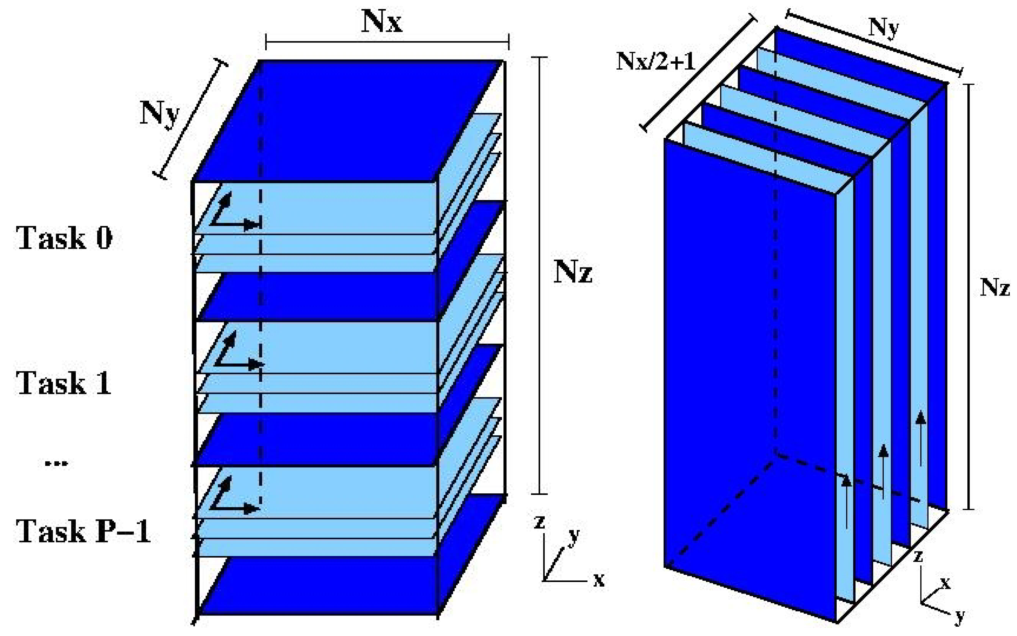
The global physical domain may be represented schematically as shown in Figure 1 left. The domain is decomposed in the vertical direction (a so-called 1D or slab decomposition) in such a way that the the vertical planes are evenly distributed to all MPI tasks (the slabs will be further decomposed into smaller domains using OpenMP, as described below). A relatively common alternative to this approach is to use the 2D “pencil” decomposition [23,25], whose performance implications were considered in M11. If P is the number of MPI tasks, there are planes of the global domain assigned as work to each task, and from the figure, it is clear that each task “owns” a slab of size points. The forward transform (for the moment, only considering MPI parallelization) consists of three main steps:
- A local 2D transform is carried out on the real physical data in each plane (lightly shaded in the figure) of the local slab, over the coordinates indicated by the arrows in Figure 1 left, which produces a partial (complex) transform that is z-incomplete because of the domain decomposition.
- Next, a global transpose (Figure 1, right) of the partially transformed data block is made so that the data becomes z- and y-complete (and, hence, x-incomplete).
- Finally, a local 1D transform is performed in the now complete z-direction for each plane of the data in the partially transformed slab (indicated by an arrow on the lightly shaded planes in Figure 1b ), producing a fully transformed data block.
Note that the total number of data points in Figure 1 left is now , and reflects the fact that the data is now complex, and that the transform satisfies the relation (assuming the data in physical space is real). However, the total amount of complex (real and imaginary) data is still the same as in the original data block. The reverse transform essentially reverses these steps to produce a real physical space field. On the CPU, the local transforms are computed using the Fast Fourier Transform (FFT) in the open source FFTW package [29,30].
The global transpose in the second step requires that all MPI tasks communicate a portion of their data to all other tasks, in an MPI all-to-all. This is handled using a non-blocking scheme detailed in [11,31], so we do not describe it further here, except to state this MPI communication is the only communication involved in the solution of the PDEs, and that it usually represents a large fraction of the global transform time, as seen below. In addition to the communication, the data local to each task must also be transposed, which can be identified as a separate computational cost. Thus, the three steps involved in computing the global FFT transform yield in turn three distinct operations whose costs (times) will be considered further below: (1) the local FFT (i.e., computation of the 2D and 1D FFTs), (2) communication (to do the global transpose), and (3) the local transpose of data.
Our previous work in M11 demonstrated how OpenMP directives enable loop-level thread parallelization of the algorithm described above to compute parallel forward transforms, its implementation in the MPI-parallelized GHOST code, and provided a detailed examination of single NUMA node performance, as well as a discussion of scaling to large core counts. This thread parallelization, on top of the MPI parallelization, results in operations performed by each thread over a smaller portion of the slab that belongs to each MPI task, and thus can be equivalent (depending on the number of MPI tasks and threads) to a pencil decomposition, in which the MPI tasks operate over slabs, and the threads over pencils in each slab. While the motivation in M11 was mainly to show the overall efficacy of this hybrid MPI-OpenMP parallelization scheme, we also described the specific directives for thread parallelization and the cache-blocking procedure used for the local transpose step. Because of the centrality of the transform, we investigate here the effect of placing as much as possible of the multidimensional Fourier transform on GPUs using CUDA, while leaving other operations done by the CFD code on the CPUs. Thus, the method we present has three layers of parallelization: MPI and OpenMP for operations done on the CPUs, and CUDA for the operations that will be moved to the GPUs.
In order to estimate the benefit of a potential GPU port of the transform, we consider timings of the basic transform operations in typical simulations at various resolutions. In Table 1 are presented fractional timing results of runs solving Equations (1)–(3) on uniform isotropic 3D grids of size for , 256, 512, and 1024. These runs were made on the NCAR-Wyoming Cheyenne cluster described in Table 2, using 4 MPI tasks per node without threading. No attempts were made to optimize MPI communication via task placement or changes to the default MPI environment. As with all subsequent timing results, the code runs in “benchmark” mode in which all computations are performed in solving the PDEs—thus, both forward and backward transforms are done—but with no intermediate I/O for time steps, and the overall time, as well as the operation (component) times, are averaged over this number of time steps. Table 1 provides the fraction of total average runtime spent on each of the transform operations identified above.
The sum of the fractional times shows that the cumulative time fraction of the distributed transform (counting FFTs, communication, and transpose) is high, and reasonably constant at about 90%, which justifies our focus on the distributed transform in isolation from the remaining computations. Indeed, the last column in Table 1 shows the maximum speed-up that could be achieved if the time to do FFTs and transposition is reduced to zero (leaving communication time the same). In terms of the component times (where represents costs not included in the transform), we can estimate this maximum possible speed-up assuming no additional costs by offloading to an accelerator as:
where the denominator approximates the aggregate runtime by using acceleration on the distributed transform, assuming and both go to 0, and that does not change by simply adding the accelerators. Here, indicates the time to compute the operation when using CPUs only, where can be communication (Comm), local FFTs (FFT), or local transpose (Transp). Since the aggregate time fraction of the transform component is so high, we can neglect . The final column in Table 1 gives this potential speed-up for each resolution.
This estimate indicates that speed-up is strongly connected to performance of the local FFT and transform relative to the communication time. While the potential speed-ups in the table may look impressive, any optimization that serves to reduce the time for the FFT and transpose on the CPU relative to the communication time will also reduce the speed-up. An obvious such optimization is threading (which is already implemented in the code, as discussed above), but we will see in Section 4 that the realized speed-ups when using GPUs are still superior to the purely CPU-based code even when multithreading is enabled.
3. CUDA Implementation
The basic CUDA implementation of the distributed transform involves interfacing directly or indirectly with CUDA code and primarily with the CUDA runtime and cuFFT libraries. We describe in the following subsections how this is accomplished in GHOST.
3.1. Preliminaries
As mentioned in Section 2, our goal for the GPU implementation of the distributed transform is to place as much work on the device as possible for as long as possible, in order to reduce the number of transfers. Of the three operations involved in the transform, the communication alone will be explicitly handled on the CPU, although future work will examine the ability of NVIDIA GPUDirectTM to at least reduce latency in transferring data directly to and from the network. The other two operations, the local transpose and local FFTs are handled with interfaces to CUDA kernels, the former to our own CUDA transpose kernel (or to the cuBLAS kernel) and the latter to the cuFFT library. GHOST (as other GFD codes) is mainly a Fortran 90/95/2003 code, so for interfacing directly or via C wrappers with CUDA we rely heavily on ISO C bindings. All calls to C or CUDA from the GHOST code occur by way of ISO C bindings which standardize the Fortran-to-C datatypes and also prevents us from having to maintain C function wrappers that accommodate compiler-specific name-mangling. A single ISO C binding interface is written for each routine called in the cuFFT, the CUDA runtime library, or made to a C function that we have written to, say, launch a CUDA kernel. An example of a binding is given in the listing below, in which the CUDA runtime function name is specified in the bind clause, and the function name called from Fortran is taken in this example to be the same:
 !****************************************************************
 ! cudaHostAlloc
 !****************************************************************
 INTEGER(C_INT) function cudaHostAlloc(buffer, isize, flags) &
    bind(C,name="cudaHostAlloc")
  USE, INTRINSIC :: iso_c_binding
  IMPLICIT NONE
  TYPE(C_PTR)        :: buffer
  INTEGER(C_SIZE_T),value  :: isize
  INTEGER(C_INT),value    :: flags
 END FUNCTION cudaHostAlloc
We note that Fortran bindings to the CUDA runtime and cuFFT libraries are available as part of Portland Group’s (PGI, [32]) CUDA Fortran language compiler. But we have a requirement to support as many compilers as possible in order to serve as broad a research community as possible, and cannot require users to use any particular compiler. For this reason, and given the ease with which they are seen to be implemented, we have implemented the required CUDA Fortran bindings in GHOST.
Many of the CUDA runtime or cuFFT library calls require parameters, or provide return values that may be examined, and are standardized. We have classified these as directives (such as cuFFT_R2C, that tells cuFFT the direction in which to compute the transform on the GPU), return codes both for cuFFT and the CUDA runtime library, and finally, device properties. The cuFFT directives and return codes are taken from the library header files, and encoded in a Fortran 90 module as parameters. Similarly, the CUDA runtime return codes are translated from the CUDA headers to a Fortran ‘enum’ type with C binding:
 ENUM, BIND(C)
  ENUMERATOR ::                              &
  cudaSuccess                =0 ,  &
  cudaErrorMissingConfiguration       =1 ,  &
  cudaErrorMemoryAllocation         =2 ,  &
  cudaErrorInitializationError        =3 ,  &
  cudaErrorLaunchFailure           =4 ,  &
  cudaErrorPriorLaunchFailure        =5 ,  &
        ...
 END ENUM
Finally, the CUDA device properties structure is also taken from the CUDA header files and made inter-operable with Fortran by encapsulating within a Fortran structure with C binding. This type may therefore be passed as a datatype to CUDA device property runtime calls. This structure takes the form:
 TYPE, BIND(C) :: cudaDevicePropG
  INTEGER   (C_INT) :: canMapHostMemory
  INTEGER   (C_INT) :: clockRate
  INTEGER   (C_INT) :: computeMode
  INTEGER   (C_INT) :: deviceOverlap
  INTEGER   (C_INT) :: integrated
  INTEGER   (C_INT) :: kernelExecTimeoutEnabled
        ...
 END TYPE cudaDevicePropG
  iret = cudaHostAlloc (planpccarr_, planszccd_, cudaHostAllocPortable)
3.2. Memory Management
lListing 1: Partial listing of the GFFTPLAN_DATA distributed plan data type. This structure is contained within the GHOST transform module. It contains the declarations for the Fortran host pointers carr, ccarr, rarr, the device pointers used in cuFFT calls, cu_dd, cu_ccd, cu_rd, and the host C_PTR blocks, pcarr, pccarr, and prarr for passing host data to CUDA runtime functions. The size variables sz* give the byte size of each host (and device) array. CUDA stream pointers and local data sizes are provided in pstream and str_*, respectively (cf., Section 3.3). Handles for the local cuFFT plans for real-to-complex (icuplanrc) and complex-to-real (icuplancr) transforms are also contained within this larger encapsulating plan.
 USE iso_c_binding
 TYPE GFFTPLAN_DATA
   COMPLEX(KIND=GP),POINTER,DIMENSION(:,:,:) :: carr,ccarr
   REAL(KIND=GP),POINTER,DIMENSION(:,:,:) :: rarr
   TYPE(C_PTR) :: pcarr,pccarr,prarr
   TYPE(C_PTR) :: cu_cd,cu_ccd,cu_rd
   TYPE(C_PTR),DIMENSION(nstreams) :: pstream
   INTEGER(C_SIZE_T) :: szcd,szccd,szrd
   INTEGER(C_SIZE_T),DIMENSION(nstreams) :: str_szcd,str_szccd,str_szrd
   INTEGER(C_SIZE_T),DIMENSION(nstreams) :: icuplanrc,icuplancr
      ...
 END TYPE GFFTPLAN_DATA
The distributed transform in GHOST is a Fortran 90 module that handles everything from set up to cleanup. The set up works in the same vein as FFTW [29,30], by creating a ’plan’ for the distributed transform. The plan contains all data required for the local FFTs, transposes and communication, and it also creates and maintains the device pointers and other data required to perform local operations on the GPU. Though in operation there are separate plans for each of the forward and backward distributed transforms, the data allocated to each plan is shared. It is also the responsibility of the GHOST plan to create the cuFFT plans that are used to carry out the local CUDA FFT transforms.
Non-device local data that are passed to CUDA runtime functions, e.g., for copying to and from device memory, are declared within the module as of TYPE(C_PTR). An example of such declarations is provided in Listing 1. The plan establishes the sizes required for each of these quantities, and these are determined by the size and datatype of the input data. There is a TYPE(C_PTR) declaration for each type of data the cuFFTs need, but the same data is used for the forward and backward transforms. They are, in all respects, standard C pointers. Each of these TYPE(C_PTR) variables is allocated on the CPU host in the creation step for a distributed plan with a call in Fortran like
 iret = cudaHostAlloc(plan%pcarr , plan%szcd , cudaHostAllocPortable)
 iret = cudaHostAlloc(plan%ppcarr , plan%szccd , cudaHostAllocPortable)
 iret = cudaHostAlloc(plan%prarr , plan%szrd , cudaHostAllocPortable)
using the cudaHostAlloc CUDA runtime function. This function allocates page-locked (pinned) memory that can be accessed directly by the GPU at higher bandwidths than, say, with malloc. In Section 3.3, we will see that this is also required for asynchronous data transfer. In all cases, the cudaHostAllocPortable flag is used to specify that the memory is pinned in all CUDA contexts. Note in this call that the C_PTR type, and the data size are contained within the distributed plan (see also Listing 1). Each cudaHostAlloc is paired with a call to cudaFreeHost in the plan’s cleanup method in order to free the host memory properly.
Once this pinned host memory is allocated, the “traditional” Fortran arrays can be associated with it for use in purely host-based operations, like MPI communication, host copies, etc. The plan therefore declares an associated Fortran pointer of the required signature (type and rank). This Fortran pointer is associated with the corresponding C_PTR block using the following ISO C binding run time call:
 CALL c_f_pointer(plan%pcarr ,plan%carr , (/Nx/2+1,Ny,kend-ksta+1/))
 CALL c_f_pointer(plan%pccarr ,plan%ccarr ,  (/Nz,Ny,iend-ista+1/))
 CALL c_f_pointer(plan%prarr ,plan%rarr , (/Nx,Ny,kend-ksta+1/))
Note that, (), and (), refer to the bounding indices of the global grid that define the work region of each MPI task, as described in Section 2: The k-bounds are required due to the z-incompleteness of the real and partially transformed data (rarr and carr), and the i-bounds are required because of the x-incompleteness of the the full complex transform (ccarr) as shown in Figure 1 left and right, respectively. Thus, while the manifestly Fortran arrays are not the central, allocated quantities used in the distributed transform method on the host, due to the interfaces with cuFFT and CUDA run time, the C_PTR host blocks lare.
Lastly, the device pointers contained within the plan are created:
 iret = cudaMalloc(plan%cu_cd , plan%szcd )
 iret = cudaMalloc(plan%cu_ccd , plan%szccd )
 iret = cudaMalloc(plan%cu_rd , plan%szrd )
These calls, and the scope of these device pointers within the transform module, allow for the persistence of the pointers until the the plan’s clean up method is called.
3.3. CUDA Streams for Overlapping Device Data Transfer and Computation
CUDA streams are used in an attempt to overlap the data transfer to the device for local cuFFT device computations [33]. The basic procedure is illustrated in Figure 2, and involves three distributed transform plan execution steps: (1) copying the data for each stream to the device asynchronously using cudaMemcpyAsync, (2) performing the local FFT on the device using the appropriate streamed cuFFT method for the local FFT being computed, and (3) having each stream copy the data back to the host again using cudaMemcpyAsync. The local cuFFT task is completed by calling the cudaStreamSynchronize, after which we are guaranteed that the computation has completed. Each of these steps is done in a “batch” process for the entire set of streams by the main thread. We emphasize that the batch processing by the main thread highlights the fact that a single GPU is bound to a single MPI task.
As mentioned in Section 3.2, the host and device storage for each of these operations, as well as the data sizes, are computed in the GHOST plan creation routine. The CUDA streams are also created there using cudaStreamCreate, and they are destroyed using a call to cudaStreamDestroy in the GHOST plan clean up method. If the local transpose operation (cf., Section 2) is performed on the device, as it is for the results presented below, execution step (3) must be postponed until after the transpose is complete.
In each batch call in execution step (2), each stream calls the appropriate cuFFT function with a cuFFT plan created for that stream. These “local” plans are created in the GHOST plan creation method; the local plan handles are carried in the GFFTPLAN_DATA in Listing 1, where icuplanrc are the plan handles for real-to-complex transforms, and icuplancr are those for complex-to-real transforms. Each of these local stream plans uses the cuFFT “advanced data layout” for batch processing of FFTs. These local plans specify the data stride between successive input and output elements, and the number of input and output elements for the FFT. Offsets for the the input and output data in the cudaMemcpyAsync in steps (1) and (3) above may also be computed in the GHOST plan creation step, and carried in the plan data for use on demand. These same offsets can be used in the calls to the cuFFT routines in execution step (2) to specify the starting location of the input and output data for a stream (see lListing A2 ). Note that the actual data passed to the cudaMemcpyAsync call and to the cuFFT routines are just the host C_PTR blocks and the device pointers discussed in Section 3.2 and stored in GFFTPLAN_DATA. Sample code for creating the real-to-complex plans is provided in lListing A1 in Appendix A.
A code sample of the three transform execution steps is provided in lListing A2 for (most of) the forward distributed transform. This code shows explicitly the “batching” of the three execution steps using CUDA streams, as well as the use of the host and device data previously discussed when interfacing with the CUDA runtime and cuFFT calls.
Additional comments about our GPU implementation are warranted. In general, the maximum number of streams allowed is set at build time. But not all GPUs support overlapping data transfer with computation as we have outlined. One should use cudaGetDeviceProperties to check the deviceOverlap field of the cudaDeviceProp structure, in order to determine if overlapping data transfer with computation is supported on a given device. If not, nstreams should be set to 1 in Listing A1. Because a single MPI task is bound to a single GPU, we cannot at this time use the multiple GPU cuFFT transforms that are available in cuFFT 8 [12]. Finally, it is worth pointing out that even when CUDA is used in the distributed transform, the code not operating on the device may still be threaded as discussed in M11. Given that the implementation binds an MPI task to a single device, the extra threading is able to exploit effectively multicore nodes that have significantly fewer GPUs than compute elements. Thus, and as previously mentioned, the code can utilize three levels of parallelization: a coarse (MPI) level, a finer-grain CPU threading level (OpenMP), and a fine grain (GPU) level. All three will be in used in Section 4.
4. Results: Scaling and Performance
A series of tests have been performed to evaluate the implementation discussed in Section 3. Most of these tests have been conducted on Oak Ridge Leadership Computing Facility’s SummitDev described in Table 2, using CUDA 9. For all tests on this system, we restrict ourselves to 16 of the 20 CPU cores on each node. Using runtime directives, the MPI tasks are placed symmetrically across the sockets, and threads from each socket are bound to their respective tasks; the GPUs are selected to optimize data transfer. When stated, for comparison purposes, we have also run on the NCAR-Wyoming Caldera analysis and visualization cluster, also described in Table 2, for which only CUDA 8 is available.
The test procedure is the same as described in Section 2, and the resulting timing output contains the total average runtime per time step (), and the component operation times for the local FFTs (), for the the MPI communication (), and for the transpose time (). The additional data transfer time (, to and from the GPUs) now also appears. These times are measured by the main thread using primarily the MPI_WTIME function, and, on the GPU, the timers wrap the entire kernel launch and execution. We compared the results of these times with Fortran, OpenMP, and CUDA timers, to verify consistency. In addition to the solver for Equations (1)–(3), we now also examine briefly the other solvers in Section 2, since we want to evaluate the performance when different sets of PDEs are used (requiring different numbers of distributed transforms). As with timings of Equations (1)–(3) presented in Section 2, we examine aggregate timings that reflect complete solutions to the equations being considered, not just of the transform kernels. Thus, component times are accumulated over both the forward and backward transforms that occur in a timestep before averaging over the number of timesteps integrated. Table 3 provides the “fiducial” runs we consider. Others, unless otherwise stated, derive from these, most often by changing task or GPU counts.
4.1. Variation with Nstreams
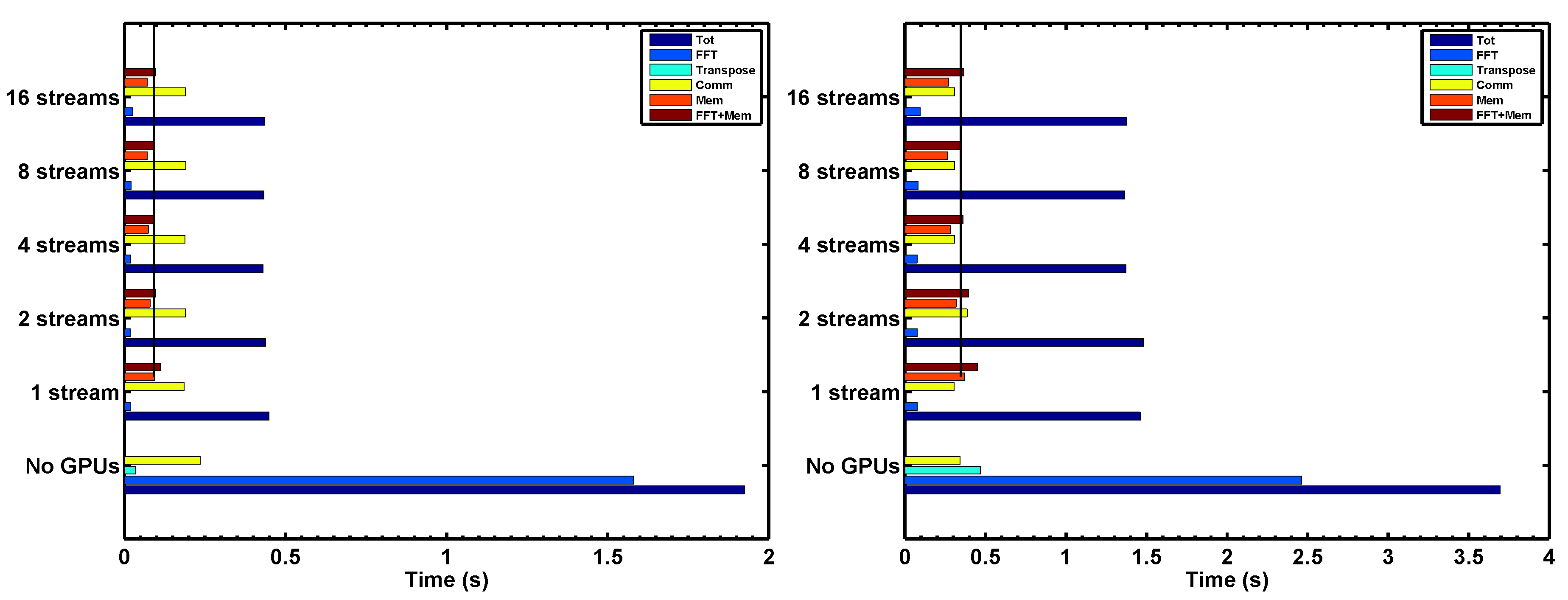
We examine first the performance of the CUDA streams for overlapping communication and computation. The pure HD equations are used here (so the temperature evolution equation Equation (2) is omitted, as is the temperature term in Equation (1)), corresponding to run 1 in Table 3. Therefore, there are two fewer (forward plus backward) distributed transforms required when compared to the full system of Equations (1)–(3) (as the HD system has one fewer nonlinear term when compared with the Boussinesq system). The grid is taken to be isotropic with points. Sixteen cores and 2 GPUs of one SummitDev (Table 2) node are used; since each GPU is bound to a single MPI task, this implies that 2 MPI tasks each with 8 threads are used (configuration 1 in Table 3). Figure 3 left shows the timings as the number of CUDA streams is varied in this system, at the bottom the times are compared to a CPU-only run. The first thing seen in the figure is that there is a good speed-up over the CPU-only case, about a factor of 4.4, achieved with the best GPU time. As expected, the FFT and local transpose times have been reduced significantly, by factors of 85 and 1300, respectively, making them nearly negligible on the GPU runs. Unexpectedly, the communication time for the identical run without GPUs is somewhat longer than for the GPU runs, and this behavior is persistent for this problem. It had been observed on the Titan development system (predecessor to SummitDev) that power supply performance on a node could explain such communication timings, at least episodically. Here, we emphasize that the slight differences in the communication timings between the GPU and CPU-only runs affect neither our subsequent results nor our conclusions.
Since both the local FFTs and the device transfers add up to the total time to compute FFTs on the GPUs, we must add the two measured times in order to determine the optimal number of streams. The and 8 runs yield nearly the same aggregated time , but gives a slightly better result, so we adopt this as the optimal number of streams for subsequent tests. The speed-up, , over the time to move data to and from the GPU and to compute the FFTs, for over that for , is . Testing on the PCIe-based Caldera system (in Table 2) for comparison (see Figure 3, right), we also find that gives the best times, but that , a larger effect due to importance of using stream optimization in the slower PCIe port. As expected, the PCIe transfer times are uniformly slower than for NVLink (see Figure 3). Because of this, the improvement when using multiple streams on the total runtime of the CFD code (when compared with the case using GPUs with 1 stream) is about on the NVLink system, versus on the PCIe system with the optimized streamed transforms. Similar results were obtained when varying for anisotropic grids with , as well as for other PDEs.
Heuristically, the aggregate speed-up, , afforded by the (streamed) GPU transforms over the CPU-only version on this system may be computed by setting the GPU times and to zero (see Figure 3), yielding
where is the remainder of the time spent on the CPU that is unrelated to distributed transform operations. For these tests, . Plugging in the values , , and for this stream test yields , which is very close to the observed speed-up. As expected, the speed-up results from the gains in the FFT computed on the GPUs, minus the cost of moving the data to the device (which is reduced by overlapping memory copies and computation using multiple streams). From this value, we also see that the speed-ups obtained are close to the maximum we can achieve (given the fraction of computations that were moved to the GPUs, see also Table 1); thus, we now consider the scaling of the method with increasing number of MPI tasks and GPUs.
4.2. Speedups on an Anisotropic Grid
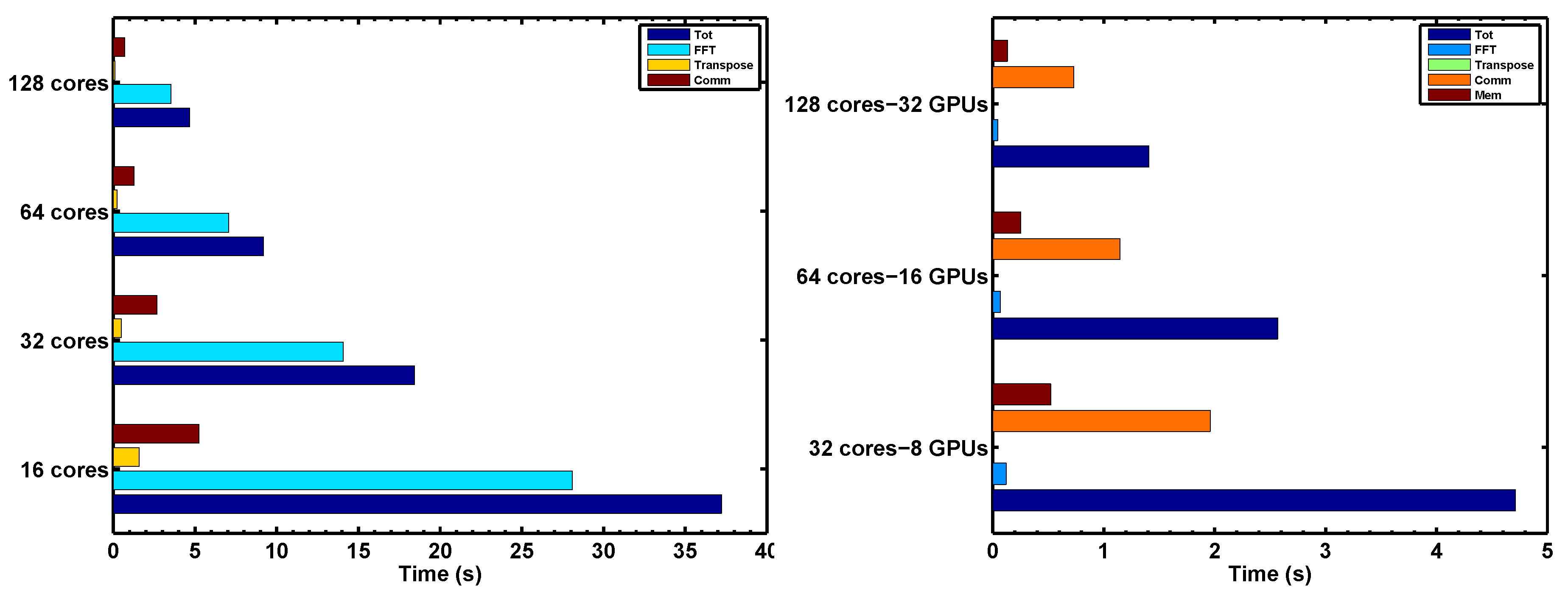
Since we are motivated strongly by the need to solve the equations for atmospheric dynamics, we consider speedup on solutions of Equations (1)–(3) on an anisotropic grid [28] (configuration 3 in Table 3). On the left in Figure 4 is a plot of CPU-only process timers, increasing the number of nodes in order to increase the number of MPI tasks. The timers indicate that each operation scales well on this system. Indeed, the average parallel efficiency , with respect to the reference aggregate time at the smallest core count , is about 98% for this problem.
In Figure 4 (right), is shown the process timers when all parallelization is turned on in configuration 3, for the SummitDev NVLink system. Comparing the aggregate speedup of the GPU runs to the CPU in Figure 4 left, we find an average speedup of over all task/node-counts. Like in Section 4.1, we observe that the FFT and local transpose times have been reduced significantly at each task/node count as well.
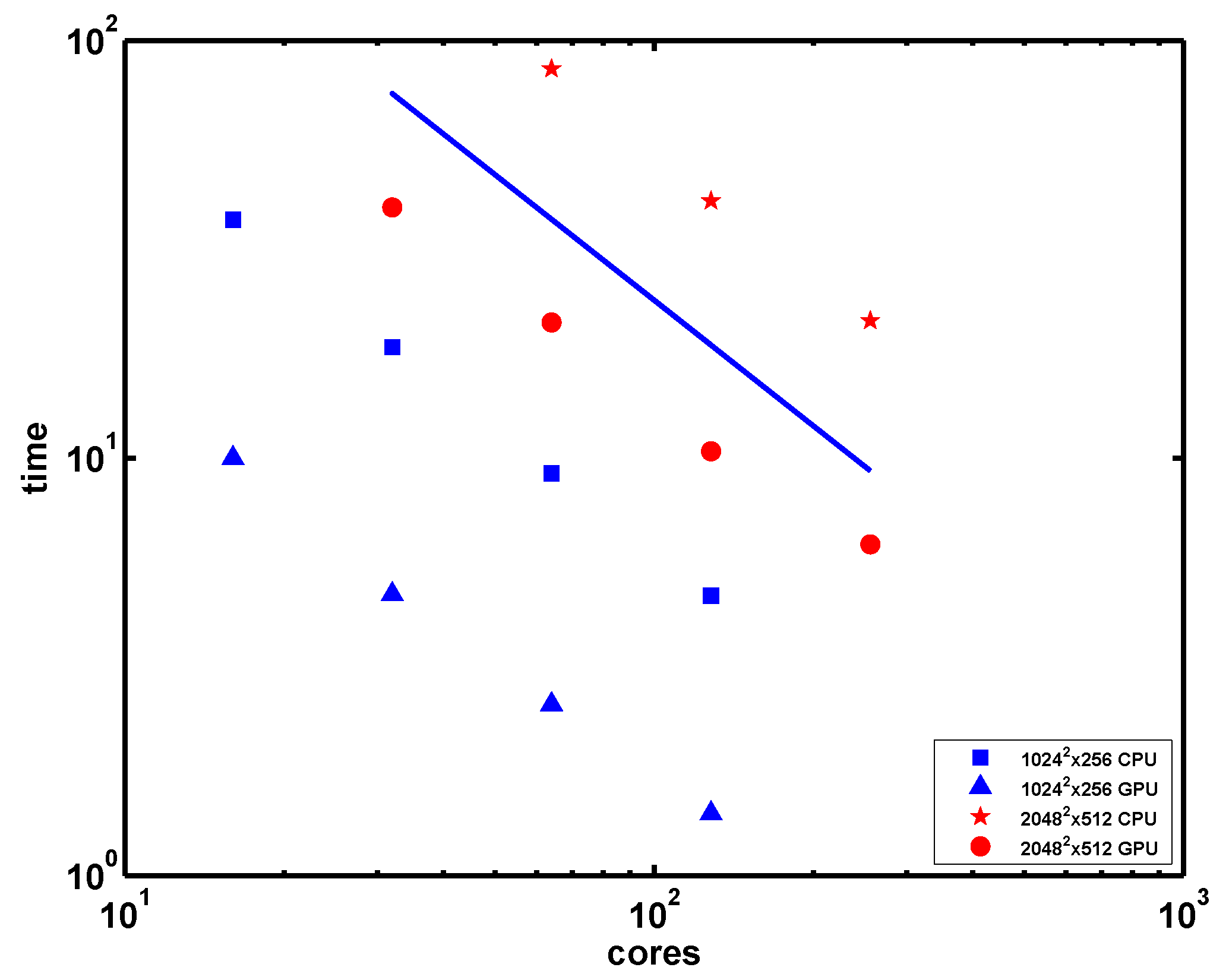
Strong scaling is perhaps seen better in the more traditional scaling plot of Figure 5, in which CPU-only and GPU total times are provided for Boussinesq runs at two different spatial resolutions (, and grid points). The simulations for the largest resolution in Figure 5 are performed using configuration 4 in Table 3. It is clear from this figure that the scaling is nearly ideal on this system for all cases considered. The average parallel efficiency of the lower resolution GPU runs based on the aggregate time is around 1, and for the higher resolution runs is .
4.3. Profiling Results
Here, we consider the GPU performance in more detail. Since the CUDA modifications apply currently only to the 3D transforms, we apply NVIDIA NVProf [34] to these CUDA kernels to examine total FlOp counts, and number of read and write transactions from/to memory. To do this, NVProf is used to examine the flop_count_sp, dram_read_transactions, and dram_write_transactions metrics. Our goal is to compute FlOp-rate and arithmetic computational intensity (CI), which is the ratio of FlOp count to the total number of memory posts and retrievals. For each metric, NVProf provides the number of invocations over all time steps and the minimum, maximum, and average of the metrics over this number for each kernel. Using run configuration 2 in Table 3, we select the average FlOp count and the average number of memory transactions for a single time step; the data is provided in Table 4. All kernels represented are from the cuFFT library, except the final transpose kernel. Note that the transpose does no computation, and only operates on memory, so it contributes nothing to the FlOp count.
The aggregate number of FlOps is given by the number of invocations times the number of total FlOp counts per invocation in Table 4, and this is GFlOps. We determine the total lcompute time for the transform as the sum of the relevant component times
and we can obtain the FlOp rate for the transform computation by dividing the FlOp count by to get 737 GFlOps/s. The nominal single-precision performance metric is 9300 GFlOps/s [35], which means we are seeing about 8% of the lnominal peak for the transform computations.
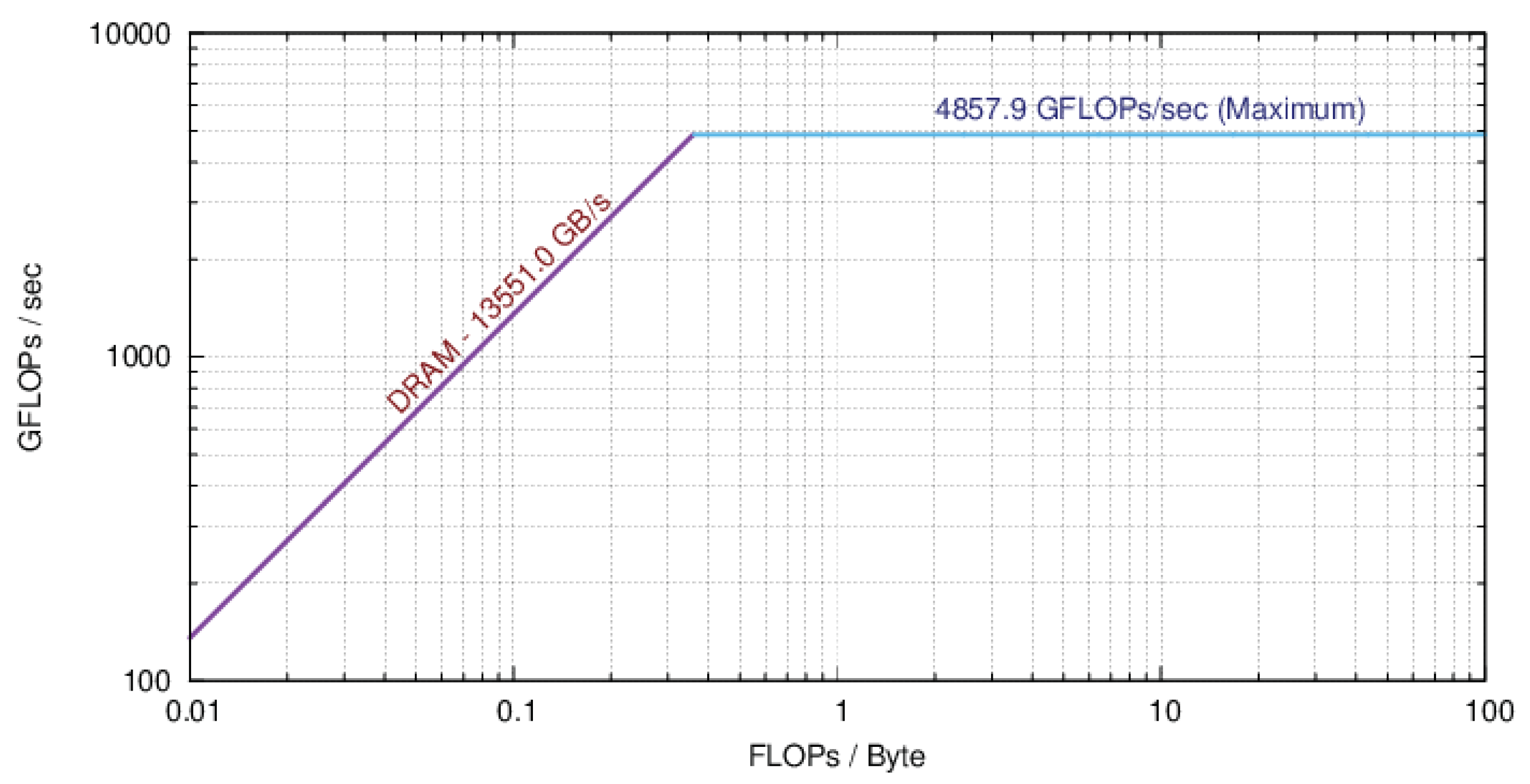
Roofline Modeling
While the nominal performance on the SummitDev P100 GPUs is 9300 GFlOps/s, this is never achievable by a real application. To determine what is achievable, we turn to a roofline model [36], namely, the Empirical Roofline Toolkit (ERT) [37] on SummitDev. This is presented in Figure 6 in a plot of attainable FlOp-rate versus computational intensity. The curve shows that below a threshold (or “machine balance”), in computational intensity, the FlOp-rate is governed by memory bandwidth, and that above machine balance, it is compute-bound, reflecting a competition between memory bandwidth, memory locality (reuse), and computation (peak FlOp-rate). ERT sweeps over a variety of micro-kernel configurations to collect its data using actual kernels while operating within lactual power environments.
Given these results, we can compute the percent-of-actual-peak performance of the GPU implementation. In Table 4, we find that the computational intensity for the transform is 12 FlOps/byte on SummitDev. From the ERT plot, Figure 6, we see that this value places us in the compute-bound region, and in the range of the realizable peak in FlOp-rate, about 4860 GFlOp/s, which is slightly greater than half of the nominal, theoretical peak. Compared with this maximum attainable value, the transform then achieves about 15% of the attainable peak performance.
4.4. Behavior of Different Solvers
In the previous subsections, we have shown that the the total runtime (and component times) for the GPU implementation follow largely the CPU-only results in their strong scaling, when solving the Boussinesq and HD equations. We expect that, as the number of nonlinear terms in the PDEs (or the number of primitive variables) is changed by a change of PDEs, the overall scaling will remain good for each PDE solver for both the CPU-only and GPU results, and we have verified this (not shown). We also expect that the speed-up in the runs with the CUDA transform over the hybrid runs for different PDEs will be similar to those in Section 4.2, another behavior that was verified by our tests. For the sake of brevity, here we summarize those studies by providing some actual measurements on the SummitDev NVLink test system.
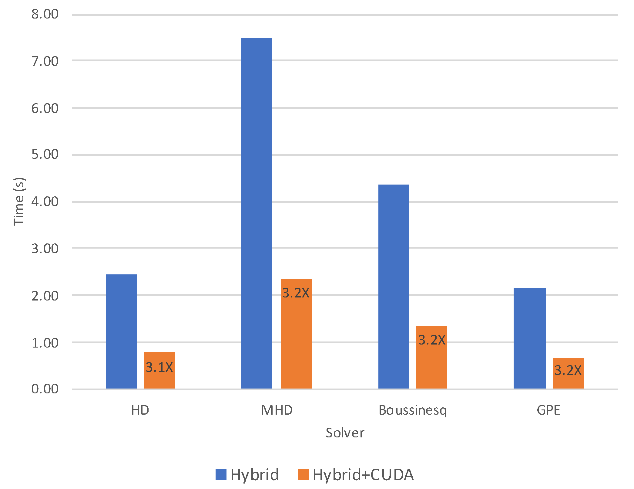
Figure 7 shows the aggregate runtimes for four different solvers. Total times are provided for a CPU-only run and a GPU run in order to compare observed speed-ups. The solvers, HD [38], MHD [39], GPE [40], and Boussinesq [19], have 3, 6, 1 complex (or 2 real), and 4 primitive fields, respectively, each solver requiring a number of distributed forward and backward transforms per time step proportional to the number of nonlinear terms in the equations (and proportional to the number of fields). The node layout is the same as that in Section 4.2, and four nodes are used for each solver, each on a grid of points. The measured speed-up of the GPU implementation of each solver over its CPU-only counterpart is indicated. All solvers see approximately the same speed-up of , similar to the anisotropic Boussinesq runs above. It is clear that neither the number of distributed transforms nor the type of grid affects the aggregate speed-up on this system. This finding, together with the scaling (admittedly to small node counts) gives us strong confidence that we will see a convincing advantage in using the CUDA implementation in our production turbulence runs on forthcoming GPU-based systems.
5. Discussion and Conclusions
We have built upon the hybrid MPI-OpenMP parallelization scheme presented in M11 to add a third level of parallelization by developing a CUDA implementation of the Geophysical High Order Suite for Turbulence (GHOST) code’s distributed multi-dimensional Fourier transform. GHOST is an accurate and highly scalable pseudospectral code that solves a variety of PDEs often encountered in studies of turbulent flows, with a special focus on the modeling of atmospheric, oceanic, and space physics turbulent flows. Whereas in M11 an isotropic grid alone was considered, in this paper, the tests admit grids with non-unit aspect ratio, a useful device for atmospheric and ocean turbulence studies. The method leverages the 1D coarse domain decomposition of the basic hybrid (CPU-only) scheme, and each MPI task now binds one GPU for additional fine grain parallelization. Our implementation hinges on the NVIDIA cuFFT advanced data layout library for device-capable local FFT routines, and depends considerably on the CUDA runtime to help manage data motion between the host and device. Implementation details have been provided that show how we integrated the access to the CUDA run time and cuFFT libraries into the code in a portable manner by using ISO bindings. We also explain how the additional parallelism leverages the existing hybrid (“CPU-only”) scheme and may be useful for multicore systems that may have fewer GPUs than cores. The resulting method is portable and provides three levels of parallelization, allowing the usage by a high-order CFD code of all CPU cores and GPUs in a system, while providing typical realizable speed-ups between 3 and 4 in tests with multiple GPUs.
Results have been presented that test the new hybrid/CUDA, GPU-based approach using, importantly, timings measuring the aggregate benefit of the implementation. As mentioned, we have demonstrated that the method can provide significant speed-up over the CPU-only computations with the addition of GPU-based computations of the distributed transform. We showed that the speed-ups are reasonably consistent with heuristics when factoring in the performance enhancement afforded by threads for the primary costs in the transform. Aside from communication, which remains a major issue in a distributed transform like ours, device data transfer times can be a significant bottleneck with this method, but we saw that NVIDIA’s NVLink effectively remedies this situation. Lastly, we examined the efficiency of the GPU implementation by examining NVProf metrics and demonstrating that we achieved about 15% of the lattainable peak of the system, based on a roofline model.
While we saw that 80–90% of total runtime is spent on the distributed transform alone, the rest of the computations could in principle be placed on the device, as well. One possibility is to use OpenACC [41], which is a directive-based programming model that allows access to the offloading device with a rich set of features particularly for GPUs. Indeed, this is the route many developers take to port legacy Fortran codes. There are several reasons why we chose not to initially adopt the OpenACC approach. First, despite early testimonials and some demonstrations of initial promise about the ease of use, we had difficulty finding clear successes in terms of aggregate performance for legacy fluid codes. Second, by the end of our development effort most compiler vendors had stopped supporting the OpenACC standard, leaving essentially a single commercial compiler vendor that does (NVIDIA via its procurement of Portland Group). Relying on a single compiler is a rather severe risk, especially in view of our requirements highlighted in Section 3.1. The implementation described herein enables the code to run with any compiler that implements OpenMP producing code that can be linked with NVCC-compiled code. That said, beginning with OpenMP 4 and and with additional features to be added to OpenMP 5 [42], it is clear that OpenMP will also provide significant support for offloading to specified “target” devices. Given the broad support by compiler vendors for OpenMP, it seems that the directive-based approach for offloading espoused by OpenACC will again be supported widely in the near future and should be considered again.
While in our implementation we transfer data from the GPU back to the host in order to handle our all-to-all communication, GPUDirectTM (see Section 3.1) may even help incentivize migrating all computations to the GPU. GPUDirectTM enables the GPU to share (page-locked) memory with network devices without having to go through the CPU using an extra copy to host memory. This should, at a minimum, reduce communication latency and may prove to be an important future path to explore.
We concentrated on the CUDA stream implementation in this version as a way to overlap data transfer with computation of the cuFFTs. In general, we see a benefit on runtimes of about 30% when using PCIe, but that this benefit is reduced when using NVLink. We have not explored whether zero-copy access of the data by the CUDA kernels can provide a larger gain when using PCIe. Since we are already using the page-locked host memory, it may be possible to see still more improved transfer speeds using zero-copy access with the CUDA Unified Memory model [43], but with the sizable improvement offered by NVLink, it seems a questionable investment. On the other hand, Unified Memory also offers the potential to considerably clean up the data management code presented in this work. We have begun such an implementation and will report on it in the future.
As parallel pseudospectral methods (as well as other high order numerical methods which require substantial communication when parallelized in distributed memory environments) are heavily used in the study of geophysical turbulence, we believe the method described here, with three levels of parallelization and with GPUs used for acceleration, can be useful for other GFD codes and for general PDEs solvers that require fast dispersion–less and dissipation–less estimations of spatial derivatives at high spatial resolutions.
Author Contributions
Conceptualization, D.R., P.D.M., A.P.; methodology, D.R., P.D.M.; validation, D.R., P.D.M., R.R.; resources, A.P., D.R., P.D.M.; writing—original draft preparation, D.R., P.D.M.; writing—review and editing, D.R., P.D.M., R.R., A.P. All authors have read and agreed to the published version of the manuscript.
Funding
D.R. acknowledges funding by Colorado State University Cooperative Institute for Research in the Atmosphere at NOAA/OAR/ESRL/Global Systems Division Award Number: NA14OAR4320125.
Acknowledgments
Computer time on Cheyenne was provided by NSF under sponsorship of the National Center for Atmospheric Research and is gratefully acknowledged. This research also used resources of the Oak Ridge Leadership Computing Facility, which is a DOE Office of Science User Facility supported under Contract DE-AC05-00OR22725. Support for AP from LASP and, in particular, from Bob Ergun, is gratefully acknowledged.
Conflicts of Interest
The authors declare no conflict of interest.
Appendix A
This Appendix contains code listings that elucidate statements made in Section 3.3. This first provides sample code for creating the complex local FFT “plans”, including the creation of the streams and the local stream cuFFT plans for 2D real-to-complex cuFFTs:
lListing A1: Partial code listing of the GHOST plan creation code showing the creation of the streams and the local stream cuFFT plans for 2D real-to-complex cuFFTs.
 DO i = 1,nstreams
   iret = cudaStreamCreate(pstream(i))
 ENDDO
  nrank= 2
 DO i = 1,nstreams
  CALL range(ista,iend,nstreams,i-1,first,last)
  issta (i) = first
  issnd (i) = last
  CALL range(ksta,kend,nstreams,i-1,first,last)
  kssta (i) = first
  kssnd (i) = last
  plan%str_szccd(i) = max(2* Nz     *Ny*(issnd(i)-issta(i)+1) &
                             *GFLOATBYTESZ,GFLOATBYTESZ)
  plan%str_szcd (i) = max(2*(Nx/2+1)*Ny*(kssnd(i)-kssta(i)+1) &
                             *GFLOATBYTESZ,GFLOATBYTESZ)
  plan%str_szrd (i) = max(   Nx   *Ny*(kssnd(i)-kssta(i)+1) &
                             *GFLOATBYTESZ,GFLOATBYTESZ)
  na   (2) = Nx      ; na   (1) = Ny;
  pinembed(2) = Nx      ; pinembed(1) = Ny*(kssnd(i)-kssta(i)+1);
  ponembed(2) = Nx/2+1    ; ponembed(1) = Ny*(kssnd(i)-kssta(i)+1);
  istr     = 1       ; idist     = Nx*Ny         ;
  ostr     = 1       ; odist     = Ny*(Nx/2+1)   ;
  iret = cufftPlanMany(plan%icuplanrc(i),nrank,na,pinembed,istr,idist, &
                     ponembed,ostr,odist,CUFFT_R2C,kssnd(i)-kssta(i)+1);
 ENDDO
The range routine in this listing computes for each stream indices that are comparable to the quantities (), and () denoting the bounds of an MPI task’s subdomain in Section 3.2, but in this case it returns the beginning and end of data chunks in each stream. The value of GFLOATBYTESZ is a constant parameter that specifies the byte size of the configurable GHOST floating type.
The second listing provides a code sample for the three transform execution steps, use of which is made in computing here just the forward distributed transform. Note that code for the computation of the local data transpose and for the final 1D batch cuFFT of the now x-complete data is omitted but indicated:
lListing A2: Partial code listing the forward GHOST transform plan execution. The three execution steps are seen clearly. The byte offsets for the input and output data are given explicitly here. Note the association of the cuFFT plans with their corresponding streams. This must be done prior to any batch cuFFT calls using a new plan so that the streamed cuFFT API can be used. The cudaMemCpyAsyncOffDev2Host is simply an ISO C-bound wrapper to the cudaMemcpyAsync that applies the offsets locating the appropriate input and output data for that batch call.
 DO i = 1,nstreams ! Associate cuFFT plans with streams
   iret = cufftSetStream(plan%icuplanr(i),pstream(i));
 END DO
 plan%rarr = real_input_data ! Copy real input data to host pointer
 DO  i = 1,nstreams ! Batch copy of input data to device
    byteoffset1 = plan%Nx*plan%Ny*(kssta(i)-ksta)*GFLOATBYTESZ
    byteoffset2 = plan%Nx*plan%Ny*(kssta(i)-ksta)*GFLOATBYTESZ
    iret = cudaMemcpyAsyncOffHost2Dev(  plan%cu_rd, & ! Dev
                             byteoffset1, & ! OFFSET Dev
                             plan%prarr, & ! Host
                             byteoffset2, & ! OFFSET Host
                  plan%str_szrd(i), pstream(i) )
 END DO
 DO  i = 1,nstreams ! Batch 2D cuFFT
    byteoffset1 = plan%Nx*plan%Ny*(kssta(i)-ksta)*GFLOATBYTESZ
    byteoffset2 = 2*(plan%Nx/2+1)*plan%Ny*(kssta(i)-ksta)*GFLOATBYTESZ
    iret = cufftExecOffR2C(plan%icuplanr(i), plan%cu\_rd, & ! Dev
                               byteoffset1, & ! OFFSET Dec
                               plan%cu_cd, & ! Dev
                               byteoffset2)    ! OFFSET Host
 END DO
 DO i = 1,nstreams ! Batch copy from device to host
  byteoffset1 = 2*(plan%Nx/2+1)*plan%Ny*(kssta(i)-ksta)*GFLOATBYTESZ
  byteoffset2 = 2*(plan%Nx/2+1)*plan%Ny*(kssta(i)-ksta)*GFLOATBYTESZ
  iret = cudaMemCpyAsyncOffDev2Host(  plan%pcarr, & ! Host
                           byteoffset1, & ! OFFSET Host
                           plan%cu_cd, & ! Dev
                           byteoffset2, & ! OFFSET Dev
                plan%str_szcd(i), pstream(i) )
 END DO
 DO  i = 1,nstreams ! Batch synchronization
    iret = cudaStreamSynchronize(pstream(i))
 END DO
 ! <Do local transpose step>
 ! <Do final batch local 1D transform in x-complete direction>
The three execution steps are seen clearly. The byte offsets for the input and output data are given explicitly. Note the association of the cuFFT plans with their corresponding streams. This must be done prior to any batch cuFFT calls using a new plan so that the streamed cuFFT API can be used. The cudaMemCpyAsyncOffDev2Host is simply an ISO C-bound wrapper to the cudaMemcpyAsync that applies the offsets locating the appropriate input and output data for that batch call.
References
- Mahrt, L. Stably Stratified Atmospheric Boundary Layers. Ann. Rev. Fluid Mech. 2014, 46, 23–45. [Google Scholar] [CrossRef] [Green Version]
- Gregg, M.; D’Asaro, E.; Riley, J.; Kunze, E. Mixing Efficiency in the Ocean. Ann. Rev. Mar. Sci. 2018, 10, 9.1–9.31. [Google Scholar] [CrossRef] [PubMed]
- Lovejoy, S.; Schertzer, D. Multifractal Cascades and the Emergence of Atmospheric Dynamics; Cambridge University Press: Cambridge, UK, 2012. [Google Scholar]
- Kalamaras, N.; Tzanis, C.G.; Deligiorgi, D.; Philippopoulos, K.; Koutsogiannis, I. Distribution of Air Temperature Multifractal Characteristics Over Greece. Atmosphere 2019, 10, 1–18. [Google Scholar] [CrossRef] [Green Version]
- Lopez, D.H.; Rabbani, M.R.; Crosbie, E.; Raman, A., Jr.; Arellano, A.F.; Sorooshian, A. Frequency and Character of Extreme Aerosol Events in the Southwestern United States: A Case Study Analysis in Arizona. Atmosphere 2016, 7, 1–13. [Google Scholar] [CrossRef] [PubMed] [Green Version]
- Cava, D.; Giostra, U.; Katul, G. Characteristics of Gravity Waves over an Antarctic Ice Sheet during an Austral Summer. Atmosphere 2015, 6, 1271–1289. [Google Scholar] [CrossRef] [Green Version]
- Medvedev, A.S.; Yigit, E.Y. Gravity Waves in Planetary Atmospheres: Their Effects and Parameterization in Global Circulation Models. Atmosphere 2019, 10, 531. [Google Scholar] [CrossRef] [Green Version]
- Zhang, Y.; Chen, X.; Dong, C. Anatomy of a Cyclonic Eddy in the Kuroshio Extension Based on High-Resolution Observations. Atmosphere 2019, 10, 553. [Google Scholar] [CrossRef] [Green Version]
- Orszag, S.A. Comparison of pseudospectral and spectral approximation. Stud. Appl. Math. 1972, 51, 253–259. [Google Scholar] [CrossRef]
- Canuto, C.; Hussaini, M.Y.; Quateroni, A.; Zang, T.A. Spectral Methods in Fluid Dynamics; Springer: New York, NY, USA, 1988. [Google Scholar]
- Mininni, P.; Rosenberg, D.; Reddy, R.; Pouquet, A. A hybrid MPI-OpenMP scheme for scalable parallel pseudospectral computations for fluid turbulence. Parallel Comput. 2011, 37, 316–326. [Google Scholar] [CrossRef] [Green Version]
- NVIDIA. cuFFT Development. 2018. Available online: https://developer.nvidia.com/cufft (accessed on 14 March 2018).
- NVIDIA. CUDA Runtime API. version v9.2.148. 2018. Available online: http://docs.nvidia.com/cuda/cuda-runtime-api/index.html (accessed on 26 July 2018).
- Ripesi, P.; Biferale, L.; Schifano, S.; Tripiccione, R. Evolution of a double-front Rayleigh-Taylor system using a graphics-processing-unit-based high-resolution thermal lattice-Boltzmann model. Phys. Rev. E 2014, 89, 043022. [Google Scholar] [CrossRef] [Green Version]
- Yokota, R.; Barba, L.A.; Narumiand, T.; Yasuoka, K. Petascale turbulence simulation using a highly parallel fast multipole method on GPUs. Comp. Phys. Commun. 2013, 184, 445–455. [Google Scholar] [CrossRef] [Green Version]
- Stürmer, M.; Götz, J.; Richter, G.; Dörfler, A.; Rüde, U. Fluid flow simulation on the Cell Broadband Engine using the lattice Boltzmann method. Comput. Math. Appl. 2009, 58, 1062–1070. [Google Scholar] [CrossRef] [Green Version]
- Govett, M.; Rosinski, J.; Middlecoff, J.; Henderson, T.; Lee, J.; MAcDonald, A.; Wang, N.; Madden, P.; Schrann, J.; Duarte, A. Parallelization and Performance of the NIM Weather Model on CPU, GPU, and MIC Processors. Bull. Am. Meteorol. Soc. 2017, 98, 2201–2213. [Google Scholar] [CrossRef] [Green Version]
- Thibault, J.C.; Senocak, I. CUDA Implementation of a Navier-Stokes solver on multi-GPU desktop platforms for incompressible flows. In Proceedings of the 47th AIAA Aerospace Sciences Meeting Including the New Horizons Forum and Aerospace Exposition, Orlando, FL, USA, 5–8 January 2009. [Google Scholar]
- Rosenberg, D.; Pouquet, A.; Marino, R.; Mininni, P.D. Evidence for Bolgiano-Obukhov scaling in rotating stratified turbulence using high-resolution direct numerical simulations. Phys. Fluids 2015, 27, 055105. [Google Scholar] [CrossRef] [Green Version]
- Ravikumar, K.; Appelhans, D.; Yeung, P. GPU acceleration of extreme scale pseudo-spectral simulations of turbulence using asynchronism. In Proceedings of the International Conference for High Performance Computing, Networking, Storage and Analysis, Denver, CO, USA, 17–22 November 2019. [Google Scholar]
- Dmitruk, P.; Wang, L.P.; Matthaeus, W.H.; Zhang, R.; Seckel, D. Scalable parallel FFT for simulations on a Beowulf cluster. Parallel Comput. 2001, 27, 1921–1936. [Google Scholar] [CrossRef]
- Kaneda, Y.; Ishihara, T.; Yokokawa, M.; Itakura, K.; Uno, A. Energy dissipation rate and energy spectrum in high-resolution DNS of turbulence in a periodic box. Phys. Fluids 2003, 15, L21–L24. [Google Scholar] [CrossRef] [Green Version]
- Yeung, P.; Donzis, D.; Sreenivasan, K. High Reynolds number simulation of turbulent mixing. Phys. Fluids 2005, 17, 081703. [Google Scholar] [CrossRef] [Green Version]
- Donzis, D.A.; Yeung, P.K.; Pekurovksy, D. Turbulence simulations at O(104) core counts. In Proceedings of the TeraGrid ’08 Conference, Las Vegas, NV, USA, 9–12 June 2008. [Google Scholar]
- Chatterjee, A.G.; Verma, M.K.; Kumarand, A.; Samtaney, R.; Hadri, B.; Khurram, R. Scaling of a Fast Fourier Transform and a pseudo-spectral fluid solver up to 196608 cores. J. Parallel Distrib. Comput. 2018, 113, 77–91. [Google Scholar] [CrossRef] [Green Version]
- Patterson, G.; Orszag, S.A. Spectral calculations of isotropic turbulence: Efficient removal of aliasing interactions. Phys. Fluids 1971, 14, 2538–2541. [Google Scholar] [CrossRef]
- Gottlieb, D.; Hussaini, M.Y.; Orszag, S.A. Spectral Methods for Partial Differential Equations; SIAM: Philadelphia, PA, USA, 1984. [Google Scholar]
- Sojovolosky, N.E.; Mininni, P.D.; Pouquet, A. Generation of turbulence through frontogenesis in sheared stratified flows. arXiv 2018, arXiv:1708.10287. [Google Scholar] [CrossRef]
- Frigo, M.; Johnson, S.G. The design and implementation of FFTW. Proc. IEEE Int. Conf. Acoust. Speech Signal Process. 1998, 3, 1381. [Google Scholar]
- Frigo, M.; Johnson, S.G. The Design and Implementation of FFTW3. Proc. IEEE 2005, 93, 216–231. [Google Scholar] [CrossRef] [Green Version]
- Gómez, D.O.; Mininni, P.D.; Dmitruk, P. Parallel simulations in turbulent MHD. Phys. Scr. 2005, T116, 123–127. [Google Scholar] [CrossRef]
- PGI. PGI CUDA Fortran Compiler. 2019. Available online: https://www.pgroup.com/resources/cudafortran.htm (accessed on 10 January 2020).
- Sanders, J.; Kandrot, E. CUDA By Example; Addison-Wesley: Boston, MA, USA, 2011. [Google Scholar]
- NVIDIA. cuDA Toolkit Documentation. 2019. Available online: https://docs.nvidia.com/cuda/profiler-users-guide/index.html (accessed on 21 October 2019).
- NVIDIA. NVIDIA Tesla P100 GPU Accelerator. 2019. Available online: https://images.nvidia.com/content/tesla/pdf/nvidia-tesla-p100-PCIe-datasheet.pdf (accessed on 1 October 2019).
- Konstantinidis, E.; Cotronis, Y. A quantitative roofline model for GPU kernel performance estimation using micro-benchmarks and hardware metric profiling. J. Parallel Distrib. Comput. 2017, 107, 37–56. [Google Scholar] [CrossRef]
- Yang, C.; Gayatri, R.; Kurth, T.; Basu, P.; Ronaghi, Z.; Adetokunbo, A.; Friesen, B.; Cook, B.; Doerfler, D.; Oliker, L.; et al. An Empirical Roofline Methodology for Quantitatively Assessing Performance Portability. In Proceedings of the 2018 IEEE/ACM International Workshop on Performance, Portability and Productivity in HPC (P3HPC), Dallas, TX, USA, 16 November 2018; pp. 14–23. [Google Scholar]
- Mininni, P.; Alexakis, A.; Pouquet, A. Nonlocal interactions in hydrodynamic turbulence at high Reynolds numbers: The slow emergence of scaling laws. Phys. Rev. E 2008, 77, 036306. [Google Scholar] [CrossRef] [Green Version]
- Mininni, P.D.; Pouquet, A. Energy spectra stemming from interactions of Alfvén waves and turbulent eddies. Phys. Rev. Lett. 2007, 99, 254502. [Google Scholar] [CrossRef] [Green Version]
- Di Leoni, P.C.; Mininni, P.D.; Brachet, M.E. Spatiotemporal detection of Kelvin waves in quantum turbulence simulations. Phys. Rev. A 2015, 92, 063632. [Google Scholar] [CrossRef] [Green Version]
- OpenACC Organization. OpenACC. 2018. Available online: https://www.openacc.org/ (accessed on 14 March 2018).
- OpenMP. OpenMP 5.0 Is a Major Leap Forward. 2019. Available online: https://www.openmp.org/press-release/openmp-5-0-is-a-major-leap-forward/ (accessed on 1 October 2019).
- NVIDIA. NVIDIA Unified Memory. 2018. Available online: https://devblogs.nvidia.com/maximizing-unified-memory-performance-cuda (accessed on 14 March 2018).
Figure 1.
Schematic of the global grid and its 1D or slab-based domain decomposition used for the global Fourier transform. (Left) The real data block in physical space, together with the decomposition of the block among MPI tasks, where the dark shaded planes indicate MPI task boundary. This decomposition highlights the z-incompleteness (and x- and y-completeness) of the physical space data. The first step of the global transform is indicated by the arrows and represents a local 2D transform in each plane of the slab owned by the task, indicated by the lightly shaded planes. (Right) The original data block has been transposed in a second global transform step, so that the partially transformed data on the left is now z- and y-complete (and x-incomplete), in order that the final step in the global transform may be done: a final 1D transform done in the direction of the arrow for the data in each of the complex (shaded) planes.

Figure 2.
Schematic of CUDA stream use to overlap data transfer from the host to the device (H2D) with cuFFT host to the device (H2D) computation. Each stream operates on only a section of the data block. The data is transferred asynchronously, and the computation starts on a stream as soon as the data transfer is complete. Black “Mcpy H2D” (“D2H”) boxes indicate copies of the data from the host to the device (or vice versa), while white “FFT” boxes correspond to the computation of the FFTs on the data available in that stream.

Figure 3.
Total time (Tot) and operation times for GPU runs (time to compute FFTs, transpose, MPI communication, memory copy from and to the GPU, and FFTs plus copies) with varying number of CUDA streams. (Left) On the NVLink system and (right) on the PCIe system (see Table 2). The minimum transfer time in both cases is seen for , and its time is indicated by the dark vertical line (compare the increase in this time for ). In the bottom of each figure, the total and component times (excluding device transfer time) are provided for a corresponding CPU-only run using the same number of MPI tasks and threads per task.

Figure 4.
Process timers (total time and operation times) for (left) CPU-only (right) GPU runs on an anisotropic grid using configuration 3 in Table 3. Note the nearly ideal scaling of each of the timers with core-count.
Figure 4.
Process timers (total time and operation times) for (left) CPU-only (right) GPU runs on an anisotropic grid using configuration 3 in Table 3. Note the nearly ideal scaling of each of the timers with core-count.

Figure 5.
Traditional strong scaling plot for anisotropic Boussinesq solves, comparing the CPU-only and GPU aggregate times for two different sets of Boussinesq runs distinguished by their resolutions (see legend), on the SummitDev NVLink system. The reference line indicates ideal scaling.
Figure 5.
Traditional strong scaling plot for anisotropic Boussinesq solves, comparing the CPU-only and GPU aggregate times for two different sets of Boussinesq runs distinguished by their resolutions (see legend), on the SummitDev NVLink system. The reference line indicates ideal scaling.

Figure 6.
lERT Roofline model of SummitDev GPUs, to show attainable peak FlOp-rate.

Figure 7.
Bar plot of the total time per time step (for the full CFD code) in CPU-only and GPU runs for each of four solvers on an isotropic grid of points with 4 nodes, 4 MPI tasks and GPUs per node, and 4 threads per MPI task. The speed-up of the GPU runs for each solver is indicated in the runtime bar for the GPU run.


Table 1.
Fraction of total runtime for each of the main operations involved in the distributed transform: FFTs (), transpose (), and communications (), for runs done with different linear resolutions N and number of cores . The remainder of the time in each run is spent on other computations. The last column gives the maximum speed-up possible if the cost for the local FFTs and transposes are driven to zero.
| N | Max Speed-Up | ||||
|---|---|---|---|---|---|
| 128 | 16 | 0.68 | 0.08 | 0.13 | 7 |
| 256 | 32 | 0.62 | 0.1 | 0.17 | 5 |
| 512 | 64 | 0.61 | 0.09 | 0.21 | 4 |
| 1024 | 128 | 0.62 | 0.08 | 0.22 | 4 |
Table 2.
Test system descriptions.
| System Name | Description |
|---|---|
| Caldera | 16 dual socket nodes, each with 2–8 core Intel Xeon E5-2670 (Sandy Bridge) CPUS, 2 NVIDIA Tesla K20Xm GPUs with PCIe Gen2 bus; FDR Mellanox Infiniband, full fat tree network. |
| Cheyenne | 145,152 dual socket nodes, each with 2–18 core Intel Xeon E5-2697 v4 (Broadwell) CPUs; enhanced hypercube interconnect. |
| SummitDev | 54 dual socket nodes, each with 2–10 core IBM Power8 CPUs, 4 NVIDIA Tesla P100 GPUs with NVLink 1.0s; EDR Infiniband, full fat tree network. |
Table 3.
Configurations for fiducial runs. Tasks and GPUs (if used) refer to the number per node, threads refers to the number per task, and streams are the number of GPU streams. The “B” designation refers to the Boussinesq equations, Equations (1)–(3), while the “H” refers to the HD equations. All runs were conducted on the SummitDev system in Table 2 and, if stated explicitly, also on the Caldera system.
| ID | Grid Size | Nodes | Tasks | Threads | GPUs | Streams |
|---|---|---|---|---|---|---|
| 1 | (H) | 1 | 2 | 8 | 2 | 1–16 |
| 2 | (B) | 1 | 4 | 5 | 4 | 8 |
| 3 | (B) | 1–8 | 4–32 | 4 | 0, 4 | 8 |
| 4 | (B) | 2–16 | 8–64 | 4 | 4 | 8 |
Table 4.
NVProf output for configuration 2 in Table 3 for each invocation of each kernel. All kernels are from cuFFT, except the transpose kernel. Computational intensity is provided in the last column. The number of invocations of each kernel in one time step of the run is 260.
Table 4.
NVProf output for configuration 2 in Table 3 for each invocation of each kernel. All kernels are from cuFFT, except the transpose kernel. Computational intensity is provided in the last column. The number of invocations of each kernel in one time step of the run is 260.
| Kernel | Avg. FlOp | Avg. Reads | Avg. Writes | CI (%) |
|---|---|---|---|---|
| spVector | 68 | |||
| spRealComplex | 78 | |||
| regular_fft | 83 | |||
| vector_fft | 68 | |||
| CUTranspose3C | 0 | – | ||
| total | 12 |
© 2020 by the authors. Licensee MDPI, Basel, Switzerland. This article is an open access article distributed under the terms and conditions of the Creative Commons Attribution (CC BY) license (http://creativecommons.org/licenses/by/4.0/).
Share and Cite
MDPI and ACS Style
Rosenberg, D.; Mininni, P.D.; Reddy, R.; Pouquet, A. GPU Parallelization of a Hybrid Pseudospectral Geophysical Turbulence Framework Using CUDA. Atmosphere 2020, 11, 178. https://doi.org/10.3390/atmos11020178
AMA Style
Rosenberg D, Mininni PD, Reddy R, Pouquet A. GPU Parallelization of a Hybrid Pseudospectral Geophysical Turbulence Framework Using CUDA. Atmosphere. 2020; 11(2):178. https://doi.org/10.3390/atmos11020178
Chicago/Turabian StyleRosenberg, Duane, Pablo D. Mininni, Raghu Reddy, and Annick Pouquet. 2020. "GPU Parallelization of a Hybrid Pseudospectral Geophysical Turbulence Framework Using CUDA" Atmosphere 11, no. 2: 178. https://doi.org/10.3390/atmos11020178
Note that from the first issue of 2016, this journal uses article numbers instead of page numbers. See further details here.