Abstract
Whistler mode waves play a major role in regulating the lifetime of trapped electrons in the Earth’s radiation belts. Specifically, interaction with whistler mode hiss waves is one of the mechanisms that maintains the slot region between the inner and outer radiation belts. The generation mechanism of hiss is a topic still under debate with at least three prominent theories present in the literature. Lightning generated whistlers in their ducted or non-ducted modes are considered to be one of the possible sources of hiss. We present a study of new observations from the Radio Receiver Instrument (RRI) on the Enhanced Polar Outflow Probe (ePOP: also known as SWARM-E). RRI consists of two orthogonal dipole antennas, which enables polarization measurements, when the satellite boresight is parallel to the geomagnetic field. Here we present 105 ePOP - RRI events from 2014–2018, in which lightning whistlers(75) and hiss waves(39) were observed. In more than 50% of those whistler observations, hiss found to co-exist. Moreover, the whistler observations are correlated with observations of wave power at the lower-hybrid resonance. The observations and a whistler mode ray-tracing study suggest that multiple-hop lightning induced whistlers can be a source of hiss and plasma instabilities in the magnetosphere.
1. Introduction
Whistler mode waves play a dominant role in Earth’s radiation belt energy dynamics. Hence lightning generated whistlers, chorus and hiss have been topics of interest for the scientific research community for more than half a century [1,2,3,4,5,6,7,8,9,10,11,12,13,14,15,16]. Chorus, a naturally occurring type of a whistler mode wave, usually exists in two frequency bands, with a gap in wave energy at around half the electron cyclotron frequency. According to the general consensus, chorus waves originate outside the plasmapause, around the magnetic equator and are driven by the pitch angle anisotropy of the energetic electron distribution [17,18,19,20,21]. Hiss, on the other hand, is less discrete in time, covers a wider bandwidth, and the source mechanism is still a topic of debate. In early work it was proposed that hiss is generated by lightning generated whistlers [6,22,23,24]. This mechanism was supported by satellite observations as well as raytracing studies. Another proposed concept posits that hiss is generated by the same nonlinear process from pitch angle anisotropy as chorus [8,25]. It has been proposed that hiss is generated in the plasma plume region and there are also hiss sources within the plasmasphere [26,27,28,29,30]. The third, and perhaps most widely accepted theory today, is that hiss is sourced from chorus waves that have undergone multiple magnetospheric reflections and propagated into the plasmasphere. This notion has also been supported by observational evidence and raytracing studies [31,32,33,34]. Chen et al. [35] identified that the plasmaspheric hiss and partly chorus being the source of low latitude ionospheric hiss. However, recently the prevalence of the chorus-to-hiss mechanism was challenged by Hartley et al. [36] who analyzed observations on the Van Allen Probes spacecraft. In all likelihood, none of the above mentioned mechanisms are mutually exclusive and there can be multiple competing sources of these waves. In this context it is also worth mentioning that lightning induced whistlers are also observed to sometimes trigger chorus waves [37].
Whistler mode waves have been observed on the ground as well as on satellites [16,28,38,39,40,41]. In this work, we present new observations of lightning whistlers and hiss observed by the enhanced Polar Outflow Probe (ePOP) Radio Receiver Instrument (RRI) [42,43,44]. RRI consists of two m orthogonal dipole antennas. This configuration allows collecting in-phase and quadrature data from 10 Hz–18 MHz. The bandwidth of the receiver is 30 kHz and the sampling rate is 62.5 kHz [42,43]. During the time from January 2014 to December 2018, RRI has observed lightning generated whistlers in 75, 4-min events. Out of those around 50% of the time whistler mode hiss was also observed. One other important observation is the presence of significant wave power at the lower hybrid (LH) resonance frequency. The LH frequency is determined by ion composition, the geomagnetic field and the plasma temperature. LH waves were first observed by Brice and Smith [45,46]. The generation of lower hybrid waves has been theoretically analyzed by Lee and Kuo [47]. Interaction between high intensity whistlers and lightning generated sferics can amplify LH noise [45,46] The presence of small scale density irregularities has also been highlighted as an important feature of LH observations [48,49]. Out of the 75 events in which we observed lightning generated whistlers, we have observed the LH waves 70% of the time showing a correlation between lightning activity and the production of LH waves.
The organization of this paper is as follows: in Section 2 we present observations of whistlers, hiss and LH resonance emissions from ePOP-RRI. In Section 3 we analyze the eccentricity of hiss for the cases presented in Section 2, followed by a ray-tracing study on the possibility of lightning generated whistlers being the source of hiss. For the raytracing study presented in this work, we used the whistler mode raytracer originally developed at Stanford University [50] and later modified at University of Colorado Denver [51]. Details of the raytracer are given in Section 4. In Section 5 we discuss the results and present conclusions in Section 6.
2. Observations
We have categorized 105 distinct observations into four cases: (1) lightning generated whistlers co-existing with hiss, (2) multi-hop ducted whistlers filling the low frequency whistler-mode band, (3) hiss observation in the absence of whistlers and (4) some special cases where observed emissions are not clearly classified. In this section we present multiple examples of the above 4 categories. Details of all observations are tabulated in Table A1, Table A2 and Table A3.
2.1. Co-Existence of Whistlers and Hiss
Figure 1 shows two spectrograms of observations made by ePOP containing whistlers with hiss. These records also include observations of wave power at the LH frequency. Figure 1a shows a two-minute record from 19 June 2015 wherein ducted whistlers are observed, with increasing dispersion with successive hops (traverses of the magnetic equator along a geomagnetic field line). The spacecraft was at . The energy from whistlers below 2.5 kHz is seen to add to pre-existing hiss wave energy in this band. In Figure 1a an emission of LH wave energy is present initially at 7 kHz, after which its frequency slightly increases and later gradually decrease to about 5 kHz at the end of the record. According to Brice and Smith [45,46], intense whistlers can excite LH waves, which is clearly observed by the higher intensities of the whistlers near and above the LH frequency. This whistler-LH interaction can be said to be the source of incoherent and broadband emissions above the LH frequency.
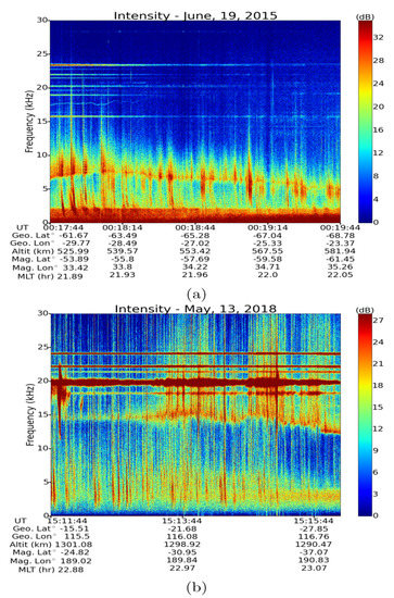
Figure 1.
Radio Receiver Instrument (RRI) frequency–time spectrograms of signal intensity of whistlers co-exisiting with hiss and lower hybrid (LH) frequency. (a) Ducted whistlers, hiss and LH frequency spectra observed on 19 June 2015. (b) Lighting generated fractional-hop whistlers, hiss and LH waves observed on 13 May 2018. In addition to the natural low frequency waves, the low frequency navy transmissions (horizontal lines within 16–24 kHz) are also visible in both spectra.
Figure 1b shows another observation of whistlers, hiss and LH frequency made by ePOP RRI on 13 May 2018. In this 4 min record fractional hop whistlers, characterized by less dispersion, are observed. This lower amount of dispersion is as expected for the spacecraft location at where ducted propagation is not expected. A hiss-like band is present throughout the record, that appears to become more intense in the final 2 mins. Compared to the case presented in Figure 1a, the hiss bandwidth is about 1 kHz higher in this observation. Moreover, the LH frequency (15 kHz) is also higher compared to the previous case (7 kHz). The frequencies of terrestrial VLF transmitters at frequencies around ∼20 kHz also exhibit spectral broadening that has been identified to be a LH resonance phenomenon [52].
2.2. Whistlers Appearing to Generate a Hiss Band
Figure 2 shows two observations of echoing ducted whistlers filling the hiss band. In Figure 2a, the observation was made by ePOP-RRI on 19 February 2014 and in addition to the hiss band (1 kHz–4 kHz) clearly shows the intensification of LH noise by the echoing whistlers at higher frequencies (5 kHz–15 kHz). In Figure 2a, echoing whistlers can be clearly identified in the 2–4 kHz frequency band and the dispersion characteristics of whistlers are visible for about 90 s. With multiple echoes, the whistlers get more dispersed and become more hiss-like. Around 14:30:14 UT, there appears to be LH plasma turbulence (a sudden intensification of the LH frequency), characterized by significant spectral broadening of the LH emission. This turbulence further intensified the LH noise around (10 kHz). This high intensified LH noise increases the entire noise level above and below the LH frequency. In the observed spectrogram, prior to the VLF turbulence (a sudden intensification in the VLF range, here we are referring to the LH turbulence, mentioned above), the noise level below LH is significantly lower compared to the noise level above it. In fact the echoing whistlers are not seen as continuous but can be said to be band rejection filtered from about 4 kHz to the LH frequency.
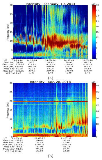
Figure 2.
RRI frequency–time spectrograms of ducted whistlers forming the hiss band. (a) Multiple echoes of ducted whistlers are forming the hiss band observed on 19 February 2014. LH plasma turbulence is observed around 14:30:14, and that increases the noise level above and beyond the LH frequency. (b) Multiple hops of ducted whistlers observed on 28 July 2018. The echoing whistlers forming the hiss band is clearly visible. In both figures the interaction of whistlers amplifying and broadening LH emissions is clearly seen.
In the spectrogram shown in Figure 2b, the echoing whistlers are filling the hiss band frequencies below 2 kHz. In this observation also, the LH frequency is present starting at 4 kHz and increasing until 7 kHz by the end of the spectrogram. Throughout the spectrogram, whistler energy intensifies the hiss frequency band. Especially in the latter half of the observation, the echoing whistler structures are clearly visible below 2 kHz. Similar to the observation made in Figure 2a, in this case also, the echoing whistlers get more dispersed with each hop. With each echo, whistlers interact with LH waves, therefore the LH noise above the LH frequency gets intensified.
2.3. Whistlers Interaction at the Lower Hybrid Resonace without Prominent Hiss
Figure 3 shows two spectrograms where there is a strong presence of LH frequency emissions without a prominent hiss band. In the spectrogram shown in Figure 3a, the LH frequency is centered around 5 kHz, and the noise level above it is significantly higher compared to the noise level below it. Although there is lightning activity present above the LH frequency, the whistler activity is lower. An important observation of this spectrogram is the absence of identifiable hiss.
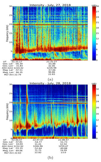
Figure 3.
RRI frequency–time spectrograms of lightning generated whistlers and lower hybrid resonance frequency without prominent hiss. (a) A short ePOP flyover observed on 27 July 2018 where interaction of lightning generated whisters amplifying LH emissions and (b) shows a more clear event observed on 28 July 2018, in which the noise level below LH frequency is significantly lower than the noise level above it.
On the observation made on 28 July 2018 shown in Figure 3b similar features are observed with whistlers driving broadening of LH noise. In this observation the LH frequency starts around 5 kHz and gradually increases up to about 8 kHz. Weaker hiss emissions are seen around 1 kHz.
2.4. Hiss Without Whistlers
Figure 4 shows an observation of plasmaspheric hiss in the absence of whistlers. The lightning activity is visible but there are no observable lightning generated whistlers. It is important to note here, that this is one of the very few clear example within 4 years worth of low frequency data of ePOP-RRI, where only hiss is visible for more than two minutes. In all the other cases there are clear signatures of whistler activity in the presence of hiss. The LH frequency is also observed in the spectrogram around 5 kHz, but the intensity of the LH is low compared to the previously presented cases. Comparing this observation with the previously presented spectrograms in Figure 1, Figure 2 and Figure 3, we can make an assertion that LH emissions are significantly reduced in the absence of whistlers.
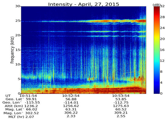
Figure 4.
RRI frequency–time spectrogram of hiss in the absence of whistlers observed on 27 April 2015. The LH frequency is visible in the spectra, but the intensity of it is low compared to the intensity of hiss.
2.5. More Complicated VLF Emissions
Figure 5 shows two examples of emissions in the ELF/VLF band that are harder to classify. The spectrogram presented in Figure 5a from April 28, 2015, shows structured emissions reminiscent of chorus. During the last 2.5 mins of the record there are rising tone structures present in the frequency range 2–3.5 kHz. In this spectrogram also, the LH frequency emission is initially visible around 6 kHz, but the intensity of the LH noise is lower compared to the cases presented before. There is a general absence of whistler activity in this observation.
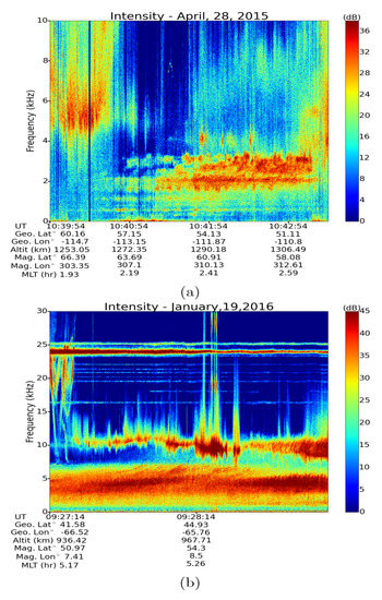
Figure 5.
RRI frequency–time spectrograms of signal intensity of low frequency waves observed by Enhanced Polar Outflow Probe (ePOP)-RRI. (a) The zoomed in spectrogram of a low frequency structures observed on 28 April 2015. There are chorus-like structures in the second portion of the spectrogram, on top of the hiss-like signals. (b) A spectrogram of low frequency noise and a strong LH frequency from 19 January 2016. The low frequency noise structure is similar to quasi-periodic (QP) emissions.
Figure 5b shows another spectrogram of low frequency and LH frequency emissions made on 19 January 2016. In this observation also, there are few whistlers observed. But, the LH frequency presented around 10 kHz is strong, and the VLF emissions extends up to 7 kHz. The VLF noise shows rising tone structures similar to quasi-periodic (QP) emissions of the type observed by Gołkowski and Inan [15]. There is some lightning activity observed around 9:27:14 UT and around 9:28:14 UT. At the time of those lightning events, the LH noise amplifies and broadens.
3. Eccentricity Analysis of Hiss
Based on the observations presented in Figure 2, echoing ducted whistlers can form a 1–2 kHz hiss-band. Depending on the number of ducted whistlers and the background noise level, the composite signal structure might look very similar to the cases presented in Figure 1. Here we perform a brief eccentricity analysis of high frequency hiss (1–2 kHz) for the sample cases presented in Figure 1, Figure 2 and Figure 4. For this analysis, we extracted amplitude maxima from the 2.5 mins observations of hiss from 1–2 kHz frequency band, and calculated the eccentricity.
As mentioned earlier, RRI consists of two orthogonal 6 m dipole antennas. When the RRI normal (boresight) is along the geomagnetic field, this configuration gives accurate polarization parameters with respect to the geomagnetic field. During all these observations the RRI normal was along the geomagnetic field. For this analysis, we have calculated the Stokes’ parameters [53] and using those, calculated the eccentricity of extracted high frequency hiss band, with the eccentricity equation given in Bass et al. [54]. Eccentricity gives a measurement of ellipticity. Our calculated eccentricity values produced a large number of data points within a small range of values. Therefore, the eccentricity presented here, is after averaging over all frequencies from 1–2 kHz and then median filtered using sets of 21 samples. Eccentricity is widely used within the magnetospheric research community than the ellipticity angle itself, hence it makes it easier to compare with the previously published data.
According to Figure 6, the eccentricities of observed hiss from all cases in this study, agree well with those calculations from previous studies [16] in which the eccentricity of magnetospheric whistler mode emissions is in the range of 0.8–0.9. The blue curve, which represents hiss in the absence of whistlers, approximately marks the center of observations. The red curves represent the two cases where the whistlers were concurrent with pre-existing hiss and the green curves represent the cases where whistlers from the upper hiss band. From the eccentricity analysis, the dashed red curve (13 May 2018) overlaps with the solid green curve (19 February 2014). Moreover, there is an overlap between the dashed green curve (28 July 2018) and the solid blue curve (27 April 2015). For the first minute of observations there is agreement between the solid red curve (19 June 2015) and the dashed green curve (28 July 2018). This analysis shows that the difference between hiss, hiss existing with whistlers, and whistlers filling the hiss band is minimal.
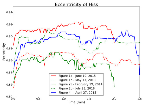
Figure 6.
Eccentricity for the hiss in the frequency band 1–2 kHz for the cases presented in Figure 1, Figure 2 and Figure 4. The eccentricity curve shown in blue is for the hiss shown in Figure 4 in the absence of whistlers. In other cases lightning generated whistlers are co-existing (or forming) hiss, therefore the eccentricity shown here, the eccentricity of whistlers is implicitly included.
4. Raytracing Results
In Figure 2 above, two cases were shown in which lightning generated ducted whistlers were echoing to fill the hiss frequency band. Table A1 and Table A2 in the Appendix A list all whistler observations made by ePOP-RRI from 2014 to 2018. The number of whistler observations were high in 2018 because in that year we requested extra ePOP observations in the very low frequency(VLF) range. In the previous years, the VLF observations were less often. We performed a raytracing study to observe the dispersion of whistlers into hiss. It is worth mentioning here that although we have made ducted whistler observations, raytracing assumes a smoothly varying background plasma and does not take special density structures such as ducts into account, causing a slight disagreement between observation and simulation background plasmaspheric conditions.
The raytracer used in this study was originally developed at the Stanford University for whistler mode raytracing in a cold (K) background magnetospheric plasma [50]. The background plasmasphere consists of electron and ions (H, He and O). This raytracer was later modified at the University of Colorado Denver, to have the option of including finite electron and ion temperature [51]. The background plasma densities used in this work were from the Global Core Plasmasphere Model (GCPM) [55].
In this work we launched waves from Hz to kHz, in Hz increments, and with initial angles from to from the vertical, and with increments from geographic latitudes to (in increments) at an altitude of 1000 km. It is important to note here that on the raytracer the launching angles are specified from the vertical axis (geographic North), hence the launching angles and the wave normal angles are the same only at the equator. At all the other latitudes the wave normal angle is different from the launching angle depending on the angle of the geomagnetic field. All waves were traced until the power of the wave reached dB from the initial power. We traced the wave normal angle along each wave trajectory.
The frequency—time spectrogram from the simulations is shown in Figure 7. The spectrogram in Figure 7 shows the simulated data points passing through a 1200 km × 1200 km square cross section, with its bottom edge located at the equator and extending upwards. The cross section is located 2000 km from the surface of the Earth. Out of 3000 echoing whistlers passing through that surface, we have picked 300 waves (interleaved by 10) to create the frequency time spectrogram in Figure 8. The frequency dispersion visible with lightning generated echoing whistlers can be seen in Figure 8, but that pattern becomes less visible after 10 s. From there onward, there is no distinguishable pattern observed and the data points are distributed randomly creating a hiss-like pattern.
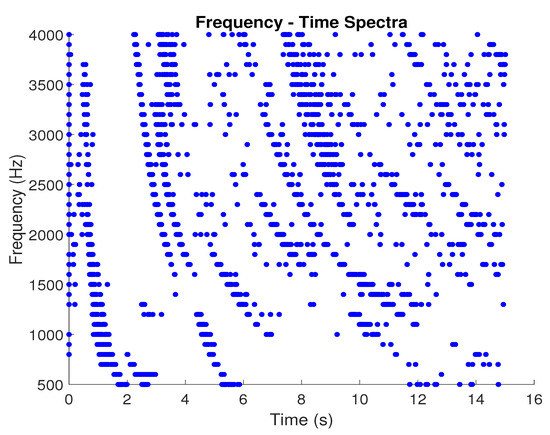
Figure 7.
Frequency-time spectrogram of simulated waves passing through a 1200 km × 1200 km section extending from the equator, which is located km away from the surface of the Earth. Out of all the waves passing though this surface only 300 waves were used to plot this spectrogram to show that the initial frequency dispersion observed with whistlers disappears after about 10 s and the observation becomes random and hiss-like.
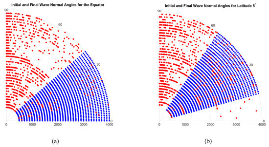
Figure 8.
In both figures, initial wave normal angles are indicated in blue and the final values are in red. Figure (a) shows the initial and final wave normal angles for the waves launched at the equator and (b) shows the initial and final wave normal angles for the waves launched at latitude . In both cases, the near-parallel wave normal angles change to more oblique values as a wave propagates. In otherwords the whistler wave normal angles become more hiss-like wave normal angles.
As mentioned above, the raytracing result is based on a smooth magnetosphere without density structures such as ducts. This causes the low frequency waves to spread-out in space with each magnetospheric reflection. Whereas the high frequency waves show multiple reflections within a small space. Therefore, as the time progresses, the reflections of low frequency waves go out of the collection region. The presence of ducts would change this result and this is the reason for the absence data points from frequencies Hz as the time progresses.
5. Discussion
In the early 1990s, researchers predicted multiple reflections of lightning generated whistlers can be a possible source of hiss [23,24]. Their conclusion was based on analysis of the wave normal angles, which showed low (<40) wave normal angles for whistlers with the wave normal angle increasing to become more characteristic of hiss-like emissions as the whistlers echo between the two hemispheres. The observed wave normal angle for hiss waves were around [23]. We revisit this concept with a raytracing study. (It deserves mentioning here that ePOP-RRI cannot measure the wave normal angles.) We also want to point out that, these final simulated wave normal angles were obtained assuming a smoothly varying magnetoplasma in the absence of density ducts. In the presence of ducts the wave normal angle distributions can vary [56].
Figure 8 presents the results from the raytracing study. Blue markers represent initial wave normal angles and red markers show the final wave normal angles for launches from the equator and from latitude. The initial wave normal angles resemble whistler wave normal angles and the final wave normal angles are more oblique representing hiss. Our wave normal angle simulation results agree with the raytracing studies and observations of Draganov et al. [23] and Sonwalkar and Inan [24]. Based on the spectrograms, eccentricity studies and raytracing studies, we see evidence for the argument that lightning generated whistlers can be a source of whistler mode hiss in the plasmasphere.
The broadband and incoherent nature of hiss waves means there is always a risk in misidentifying noise, interference, or electrostatic waves as a magnetospheric hiss emission. Unlike many studies of satellite data were waves are automatically identified using often simple predefined criteria, the records classified herein have all been visually inspected by the authors. The majority of magnetospheric hiss wave energy has been previously observed to be between and [24]. In Table A1 and Table A2 we have indicated the L values for each of our observations, and a histogram of those values is shown in Figure 9. For the observations made between latitudes , there were no L shell mappings, because of the diffusive region. According to Figure 9, the majority of our hiss observations were made between . Although our results are based on a limited number of observations, those agree with most of the previous findings and reinforcing that we are considering the same type of magnetospheric hiss.
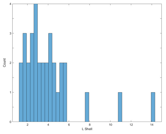
Figure 9.
Occurrence of hiss with respect to the L value is shown in this figure. The majority of the observations were made with in .
Table A3 presents the ePOP events where hiss was observed in the absence of whistlers within the 2014–2018 period. The number of observations of hiss without whistlers is less than the co-existence of both. Also, once hiss is generated it can exist for a long period of time; hence, the source signals are not present by the time of observation.
Figure 10 shows a map indicating all the observation locations listed in Table A1, Table A2 and Table A3. In Figure 10 markers in red indicate the locations where hiss coexisting with whistlers, green indicates the locations of whistlers in the absence of hiss and blue markers show the locations where hiss was observed without whistlers. Significant number of events are from the North American sector, because at the time the authors requested more low frequency ePOP passes over North America. We have not shown the geomagnetic footprint here since we have observed a mix of ducted and non-ducted whistlers.
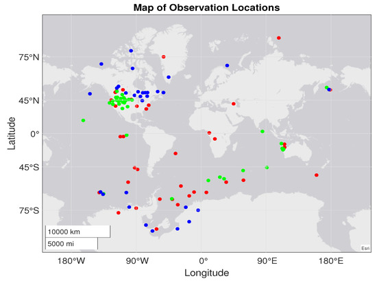
Figure 10.
A map showing the geographic locations of ePOP events. Red markers indicate events where whistlers coexist with hiss, green markers show the locations where whistlers were observed but no hiss, and blue markers represent the events hiss was observed but no whistlers.
We also observed prominent emissions at the LH frequency in our observations. Our observations show a close correlation between the occurrence of whistlers and the occurrence of LH emissions. Both LH frequency and whistlers are triggered by lightning strokes therefore, when there is high lightning activity, there is a high probability of generating both whistlers and LH waves. Interaction between high intensity whistlers and LH waves increases the wave energy level above the LH frequency. In the presence of strong LH emissions, the amount of lightning whistler energy observed below the LH frequency is low. With each bounce whistlers are observed to lose intensity due to the interaction with LH emissions.
In any single point measurement, it is often very difficult to discriminate between generation effects and propagation effects when two types of waves are observed. For example, the coexistence of hiss and whistlers could be facilitated by both of these waves being guided by magnetospheric ducts. On the other hand, wave-particle interactions can drive frequency-dependent wave amplification and wave generation. We believe that the observations presented here give evidence for the latter. In this context, linear growth from cyclotron resonance with the energetic electron distribution in the 1–4 kHz band, coupled with LH resonance driven growth at 5 kHz–15 kHz best explains the observations. As an example of these processes occurring concurrently, a closer look at Figure 3 shows that spectral broadening of a VLF transmitter signal just below 25 kHz is concurrent with growth of the hiss band below 3 kHz. There is also a clear role for cold plasma density irregularities since guiding of waves by large scale structures (ducts) favors cyclotron growth while small scale irregularities are favorable to LH instabilities. The realistic plasmasphere will host both types of irregularities concurrently and full wave simulations in multiple dimensions may be needed to model both mechanisms simultaneously.
6. Conclusions
In this work we presented new VLF observations by the Radio Receiver Instrument (RRI) on the Enhanced Polar Outflow Probe (e-POP or SWARM-E). In several years of data, 51% of the time whistler mode hiss is observed to coexist with lightning induced whistlers. Moreover, in individual cases the hiss band can be seen to be partially or fully composed of high order whistler echoes. Out of those 75 whistler observations, 70% of the time we observed the lower hybrid (LH) resonance as well. We presented cases where whistlers co-existing with hiss, whistlers forming the hiss band, whistlers and LH emissions without hiss and hiss in the absence of whistlers. Our observations suggested a strong probability of observing whistlers, LH and hiss simultaneously.
The eccentricity analysis for hiss showed no difference in eccentricity between different categories of hiss suggesting that whether the observed hiss is composed of multiple echoes of ducted whistlers or in the absence of whistlers, the wave propagation properties are similar. Frequency-time spectrograms produced from our raytracing study also suggested that whistlers show a more hiss-like behavior after multiple reflections.
Strong interactions between whistlers and LH noise were also observed wherein LH emissions would gain in intensity and bandwidth when a whistler was present. The stronger the interaction between whistlers and LH emission, the less whistler energy was observed below the LH frequency, hence a band-rejection filter effect between the highest hiss frequencies and the LH frequency. Our observations suggest that the amplitude of observed lightning induced whistlers is frequency dependent and depends on wave-particle interactions in the hiss band and LH band. The notion of lightning whistlers not only experiencing, but also driving these interactions and generating the other waves is worthy of renewed theoretical consideration.
7. Materials and Methods
All data used in this paper are publicly available from the e-POP data repository at https://epop-data.phys.ucalgary.ca/ [57]. Observation data were analyzed with the Python software and the scripts will be available upon request.
Author Contributions
Conceptualization, A.M., M.G. and G.H., methodology M.G. and A.M., data curation and software, A.M., writing–original draft preparation A.M. and M.G., writing–review and editing, A.M., M.G. and G.H., funding acquisition G.H. and M.G. All authors have read and agreed to the published version of the manuscript.
Funding
This research was funded by Canadian Space Agency under grant 16SUSTSSPI, e-POP/SWARM-E satellite mission is funded by Natural Science and Engineering Research Council under Discovery Grant RGPIN/06069-2014, and the European Space Agency (ESA) under the Third Party Mission Program. MG is funded by National Aeronautics and Space Administration(NASA) grant 80NSSC19K0264.
Acknowledgments
Authors would like to acknowledge Andrew Yau at the University of Calgary, the principal investigator of e-POP.
Conflicts of Interest
The authors declare no conflict of interest.
Abbreviations
The following abbreviations are used in this manuscript:
| RRI | Radio Receiver Instrument |
| e-POP | Enhanced Polar Outflow Probe |
| GCPM | Global Core Plasmasphere Model |
Appendix A
Appendix A.1.

Table A1.
List of events in which whistlers were observed and indicating whether the hiss and or the lower hybrid resonance was observed too.
Table A1.
List of events in which whistlers were observed and indicating whether the hiss and or the lower hybrid resonance was observed too.
| Number | Date | Pass Start Time (UT) | Altitude (km) | L-shell | Ducted? | Hiss? | LHR? |
|---|---|---|---|---|---|---|---|
| 1 | 2014-Feb-19 | 14:29:14 | 600 | 2.72 | Y | Y | Y |
| 2 | 2014-Feb-22 | 14:29:14 | 500 | 5.34 | Y | N | Y |
| 3 | 2014-Aug-03 | 03:49:09 | 884 | 4.49 | Y | Y | Y |
| 4 | 2014-Oct-11 | 02:43:08 | 1282 | 2.60 | Y | N | N |
| 5 | 2015-May-19 | 22:14:44 | 443 | 5.35 | Y | Y | Y |
| 6 | 2015-Jun-19 | 00:17:44 | 553 | 3.26 | Y | Y | Y |
| 7 | 2015-Jun-29 | 06:36:14 | 800 | 4.79 | Y | Y | Y |
| 8 | 2015-Jul-03 | 05:44:13 | 950 | 5.32 | Y | N | N |
| 9 | 2016-Jan-17 | 13:23:04 | 877 | 2.04 | N | N | N |
| 10 | 2016-Jan-22 | 20:11:04 | 500 | 1.51 | N | N | N |
| 11 | 2016-Mar-08 | 14:00:29 | 1352 | 2.17 | N | N | N |
| 12 | 2016-Oct-21 | 10:18:44 | 836 | 3.92 | Y | Y | Y |
| 13 | 2017-Jun-13 | 00:14:44 | 358 | 3.59 | Y | N | Y |
| 14 | 2017-Jun-21 | 04:02:14 | 477 | 5.53 | Y | Y | Y |
| 15 | 2017-Jun-22 | 18:58:14 | 633 | 5.10 | Y | Y | Y |
| 16 | 2018-Mar-07 | 15:19:44 | 651 | 2.60 | N | N | Y |
| 17 | 2018-Mar-10 | 11:37:44 | 1150 | 1.65 | N | N | Y |
| 18 | 2018-Mar-12 | 14:59:13 | 530 | 2.37 | N | N | Y |
| 19 | 2018-Mar-13 | 00:50:43 | 900 | – | N | Y | Y |
| 20 | 2018-Apr-28 | 21:30:14 | 1300 | 3.85 | N | N | Y |
| 21 | 2018-Apr-30 | 19:00:14 | 1311 | 4.18 | N | N | Y |
| 22 | 2018-May-10 | 09:08:14 | 550 | 14.29 | N | Y | Y |
| 23 | 2018-May-12 | 15:36:14 | 1300 | – | N | N | Y |
| 24 | 2018-May-13 | 15:11:44 | 1300 | 1.60 | N | Y | Y |
| 25 | 2018-May-14 | 06:00:44 | 1057 | 2.42 | N | Y | Y |
| 26 | 2018-May-15 | 03:53:44 | 1074 | 2.90 | N | Y | Y |
| 27 | 2018-May-19 | 05:37:44 | 1140 | 2.86 | N | Y | Y |
| 28 | 2018-May-19 | 14:24:44 | 1260 | 1.59 | N | Y | Y |
| 29 | 2018-May-24 | 01:50:14 | 1250 | 2.33 | N | Y | Y |
| 30 | 2018-May-25 | 01:25:14 | 1260 | 2.28 | N | Y | Y |
| 31 | 2018-Jun-04 | 09:47:14 | 381 | 3.41 | Y | Y | Y |
| 32 | 2018-Jun-19 | 05:09:44 | 370 | 4.15 | Y | Y | N |
| 33 | 2018-Jun-20 | 04:44:48 | 380 | 3.72 | Y | Y | Y |
| 34 | 2018-Jun-20 | 06:24:42 | 350 | 7.77 | Y | Y | Y |
| 35 | 2018-Jun-29 | 02:40:47 | 372 | 5.47 | Y | Y | N |
| 36 | 2018-Jun-30 | 00:35:44 | 373 | 4.36 | N | Y | N |
| 37 | 2018-Jun-30 | 02:15:46 | 500 | 4.36 | N | Y | N |
| 38 | 2018-Jul-14 | 23:25:41 | 928 | 4.21 | Y | N | Y |
| 39 | 2018-Jul-21 | 00:42:15 | 1290 | – | N | Y | Y |
| 40 | 2018-Jul-21 | 07:10:15 | 1128 | 1.94 | Y | Y | Y |
| 41 | 2018-Jul-21 | 22:50:45 | 1096 | 1.92 | N | Y | N |
| 42 | 2018-Jul-22 | 06:48:45 | 1190 | 1.70 | N | Y | Y |
| 43 | 2018-Jul-22 | 08:43:45 | 1285 | – | N | Y | N |
| 44 | 2018-Jul-22 | 23:52:15 | 1286 | – | N | Y | Y |
| 45 | 2018-Jul-23 | 06:23:45 | 1228 | 1.53 | N | Y | Y |
Table A2.
List of events in which whistlers were observed and indicating whether the hiss and or the lower hybrid resonance was observed too.
Table A2.
List of events in which whistlers were observed and indicating whether the hiss and or the lower hybrid resonance was observed too.
| Number | Date | Pass Start Time (UT) | Altitude (km) | L-shell | Ducted? | Hiss? | LHR? |
|---|---|---|---|---|---|---|---|
| 46 | 2018-Jul-23 | 08:18:45 | 1277 | – | N | Y | N |
| 47 | 2018-Jul-24 | 07:53:44 | 1270 | – | N | N | N |
| 48 | 2018-Jul-27 | 21:31:17 | 1225 | 4.12 | Y | N | Y |
| 49 | 2018-Jul-28 | 08:08:15 | 785 | 10.87 | N | Y | Y |
| 50 | 2018-Jul-28 | 21:05:17 | 1264 | 3.47 | Y | Y | Y |
| 51 | 2018-Jul-28 | 22:46:47 | 1269 | 2.93 | Y | N | Y |
| 52 | 2018-Aug-10 | 06:01:45 | 660 | 2.56 | N | N | Y |
| 53 | 2018-Aug-12 | 06:52:15 | 563 | 3.23 | N | N | Y |
| 54 | 2018-Aug-13 | 06:26:45 | 570 | 2.78 | N | Y | Y |
| 55 | 2018-Aug-14 | 09:15:15 | 736 | 1.25 | N | N | N |
| 56 | 2018-Aug-26 | 22:32:15 | 800 | 1.28 | Y | Y | Y |
| 57 | 2018-Aug-29 | 04:45:45 | 336 | 3.25 | Y | N | Y |
| 58 | 2018-Aug-30 | 04:19:15 | 335 | 3.03 | N | N | Y |
| 59 | 2018-Sep-01 | 03:27:45 | 331 | 2.82 | N | N | Y |
| 60 | 2018-Oct-05 | 09:32:14 | 1293 | 2.72 | N | N | Y |
| 61 | 2018-Oct-07 | 08:41:14 | 1291 | 3.35 | Y | Y | Y |
| 62 | 2018-Oct-10 | 09:05:13 | 1259 | 2.58 | Y | N | Y |
| 63 | 2018-Oct-11 | 08:39:13 | 1240 | 2.46 | N | N | Y |
| 64 | 2018-Oct-12 | 08:13:14 | 1240 | 2.78 | N | N | Y |
| 65 | 2018-Oct-13 | 07:48:14 | 1240 | 3.06 | N | N | Y |
| 66 | 2018-Oct-14 | 09:05:14 | 1235 | 3.09 | Y | Y | Y |
| 67 | 2018-Oct-15 | 08:38:14 | 1206 | 2.70 | N | N | Y |
| 68 | 2018-Oct-16 | 08:12:14 | 1180 | 2.57 | N | N | Y |
| 69 | 2018-Oct-20 | 08:12:14 | 1135 | 2.82 | Y | N | Y |
| 70 | 2018-Oct-21 | 07:45:14 | 1090 | 2.59 | Y | N | Y |
| 71 | 2018-Oct-22 | 07:20:14 | 1107 | 3.26 | N | N | Y |
| 72 | 2018-Oct-26 | 07:18:14 | 977 | 2.51 | Y | N | N |
| 73 | 2018-Oct-28 | 06:26:14 | 1033 | 4.5 | Y | Y | N |
| 74 | 2018-Nov-07 | 05:33:14 | 650 | 2.05 | N | N | N |
| 75 | 2018-Dec-26 | 22:21:44 | 616 | – | N | N | N |
| Total | 75 | 39 | 57 | ||||
| Percentage | % | 52 | 76 |
Table A3.
List of events in which hiss was observed in the absence of whistlers.
Table A3.
List of events in which hiss was observed in the absence of whistlers.
| Number | Date | Pass Start Time (UT) |
|---|---|---|
| 1 | 2014-Feb-08 | 23:58:14 |
| 2 | 2014-Feb-09 | 00:00:00 |
| 3 | 2014-Feb-20 | 14:29:14 |
| 4 | 2014-May-27 | 23:42:00 |
| 5 | 2014-Jun-21 | 06:15:13 |
| 6 | 2015-Apr-24 | 11:27:54 |
| 7 | 2015-Apr-27 | 10:51:54 |
| 8 | 2016-Apr-15 | 14:20:44 |
| 9 | 2016-Sep-28 | 02:35:14 |
| 10 | 2017-Jan-19 | 11:02:13 |
| 11 | 2017-Feb-01 | 08:10:43 |
| 12 | 2017-Feb-03 | 07:28:43 |
| 13 | 2017-Feb-04 | 07:06:43 |
| 14 | 2017-Feb-05 | 06:45:43 |
| 15 | 2017-Mar-04 | 11:03:43 |
| 16 | 2017-Mar-30 | 14:10:13 |
| 17 | 2017-Jun-19 | 04:46:14 |
| 18 | 2017-Jul-11 | 23:41:14 |
| 19 | 2017-Aug-28 | 04:27:42 |
| 20 | 2017-Sep-07 | 02:17:14 |
| 21 | 2017-Oct-16 | 06:06:44 |
| 22 | 2017-Oct-16 | 07:47:54 |
| 23 | 2017-Oct-18 | 07:00:04 |
| 24 | 2017-Oct-25 | 05:55:14 |
| 25 | 2017-Dec-19 | 05:01:14 |
| 26 | 2018-Jun-02 | 07:11:14 |
| 27 | 2018-Jun-03 | 05:06:14 |
| 28 | 2018-Jun-10 | 05:32:44 |
| 29 | 2018-Jun-26 | 02:15:24 |
| 30 | 2018-Jun-26 | 03:55:54 |
References
- Bortnik, J.; Thorne, R.M.; Meredith, N.P. Modeling the propagation characteristics of chorus using CRRES suprathermal electron fluxes. J. Geophys. Res. Space Phys. 2007, 112. [Google Scholar] [CrossRef]
- Horne, R.B.; Thorne, R.M. Potential waves for relativistic electron scattering and stochastic acceleration during magnetic storms. Geophys. Res. Lett. 1998, 25, 3011–3014. [Google Scholar] [CrossRef]
- Horne, R.B.; Meredith, N.P.; Thorne, R.M.; Heynderickx, D.; Iles, R.H.A.; Anderson, R.R. Evolution of energetic electron pitch angle distributions during storm time electron acceleration to megaelectronvolt energies. J. Geophys. Res. Space Phys. 2003, 108. [Google Scholar] [CrossRef]
- Horne, R.B.; Thorne, R.M.; Glauert, S.A.; Albert, J.M.; Meredith, N.P.; Anderson, R.R. Timescale for radiation belt electron acceleration by whistler mode chorus waves. J. Geophys. Res. Space Phys. 2005, 110. [Google Scholar] [CrossRef]
- Lyons, L.R.; Lee, D.Y.; Thorne, R.M.; Horne, R.B.; Smith, A.J. Solar wind-magnetosphere coupling leading to relativistic electron energization during high-speed streams. J. Geophys. Res. Space Phys. 2005, 110. [Google Scholar] [CrossRef]
- Meredith, N.P.R.B.H.; Clilverd, M.A.; Horsfall, D.; Thorne, R.M.; Anderson, R.R. Origins of plasmaspheric hiss. Geophys. Res. 2006, 111, A09217. [Google Scholar] [CrossRef]
- Miyoshi, Y.; Morioka, A.; Misawa, H.; Obara, T.; Nagai, T.; Kasahara, Y. Rebuilding process of the outer radiation belt during the 3 November 1993 magnetic storm: NOAA and Exos-D observations. J. Geophys. Res. Space Phys. 2003, 108. [Google Scholar] [CrossRef]
- Nakamura, S.; Omura, Y.; Summers, D.; Kletzing, C.A. Observational evidence of the nonlinear wave growth theory of plasmaspheric hiss. Geophys. Res. Lett. 2016, 43, 10040–10049. [Google Scholar] [CrossRef]
- Smith, A.J.; Horne, R.B.; Meredith, N.P. Ground observations of chorus following geomagnetic storms. J. Geophys. Res. Space Phys. 2004, 109. [Google Scholar] [CrossRef]
- Spasojevíc, M.; Inan, U.S. Ground based VLF observations near L = 2.5 during the Halloween 2003 storm. Geophys. Res. Lett. 2005, 32. [Google Scholar] [CrossRef]
- Summers, D.; Thorne, R.M.; Xiao, F. Relativistic theory of wave-particle resonant diffusion with application to electron acceleration in the magnetosphere. J. Geophys. Res. Space Phys. 1998, 103, 20487–20500. [Google Scholar] [CrossRef]
- Thorne, R.M.; O’Brien, T.P.; Shprits, Y.Y.; Summers, D.; Horne, R.B. Timescale for MeV electron microburst loss during geomagnetic storms. J. Geophys. Res. Space Phys. 2005, 110. [Google Scholar] [CrossRef]
- Varotsou, A.; Boscher, D.; Bourdarie, S.; Horne, R.B.; Glauert, S.A.; Meredith, N.P. Simulation of the outer radiation belt electrons near geosynchronous orbit including both radial diffusion and resonant interaction with Whistler-mode chorus waves. Geophys. Res. Lett. 2005, 32. [Google Scholar] [CrossRef]
- Wang, C.; Xiao, F.; Wang, Y.; Yue, C. The relations between magnetospheric chorus and hiss inside and outside the plasmasphere boundary layer: Cluster observation. Geophys. Res. 2011, 116, A07221. [Google Scholar] [CrossRef]
- Gołkowski, M.; Inan, U.S. Multistation observations of ELF/VLF whistler mode chorus. J. Geophys. Res. Space Phys. 2008, 113. [Google Scholar] [CrossRef]
- Hosseini, P.; Gołkowski, M.; Turner, D.L. Unique concurrent observations of whistler mode hiss, chorus, and triggered emissions. J. Geophys. Res. Space Phys. 2017, 122, 6271–6282. [Google Scholar] [CrossRef]
- Lyons, L.R.; Thorne, R.M. Equilibrium structure of radiation belt electrons. J. Geophys. Res. (1896-t5-1977) 1973, 78, 2142–2149. [Google Scholar] [CrossRef]
- Omura, Y.; Hikishima, M.; Katoh, Y.; Summers, D.; Yagitani, S. Nonlinear mechanisms of lower-band and upper-band VLF chorus emissions in the magnetosphere. J. Geophys. Res. Space Phys. 2009, 114. [Google Scholar] [CrossRef]
- Omura, Y.; Nunn, D. Triggering process of whistler mode chorus emissions in the magnetosphere. J. Geophys. Res. Space Phys. 2011, 116. [Google Scholar] [CrossRef]
- Gołkowski, M.; Gibby, A.R. On the conditions for nonlinear growth in magnetospheric chorus and triggered emissions. Phys. Plasmas 2017, 24, 092904. [Google Scholar] [CrossRef]
- Gołkowski, M.; Harid, V.; Hosseini, P. Review of Controlled Excitation of Non-linear Wave-Particle Interactions in the Magnetosphere. Front. Astron. Space Sci. 2019, 6, 2. [Google Scholar] [CrossRef]
- Smith, R.L.; Angerami, J.J. Magnetospheric properties deduced from OGO 1 observations of ducted and nonducted whistlers. Geophys. Res. 1968, 73, 1. [Google Scholar] [CrossRef]
- Draganov, A.B.U.S.I.; Sonwalkar, V.S.; Bell, T.F. Whistlers and plasmaspheric hiss: Wave directions and three-dimensional propagation. Geophys. Res. 1993, 98, 11401. [Google Scholar] [CrossRef]
- Sonwalkar, V.; Inan, U. Lightning as an embryonic source of VLF hiss. J. Geophys. Res. Space Phys. 1989, 94, 6986–6994. [Google Scholar] [CrossRef]
- Omura, Y.; Nakamura, S.; Kletzing, C.A.; Summers, D.; Hikishima, M. Nonlinear wave growth theory of coherent hiss emissions in the plasmasphere. J. Geophys. Res. Space Phys. 2015, 120, 7642–7657. [Google Scholar] [CrossRef]
- Cornilleau-Wehrlin, N.; Gendrin, R.; Lefeuvre, F.; Parrot, M.; Grard, R.; Jones, D.; Bahnsen, A.; Ungstrup, E.; Gibbons, W. VLF electromagnetic waves observed onboard GEOS-1. Space Sci. Rev. 1978, 22, 371–382. [Google Scholar] [CrossRef]
- Hayakawa, M.; Ohmi, N.; Parrot, M.; Lefeuvre, F. Direction finding of ELF hiss emissions in a detached plasma region of the magnetosphere. Geophys. Res. 1986, 91, 135–141. [Google Scholar] [CrossRef]
- Parrot, M.; Lefeuvre, F. Statistical study of the propagation characteristics of ELF hiss observed on GEOS-1, inside and outside the plasmasphere. Ann. Geophys. Ser. 1986, A4, 363–384. [Google Scholar]
- Russell, C.T.; Smith, E.J. OGO 3 observations of ELF noise in the magnetosphere: 1. Spatial extent and frequency of occurrence. Geophys. Res. 1969, 74, 755–777. [Google Scholar] [CrossRef]
- Laakso, H.; Santolik, O.; Horne, R.; Kolmasová, I.; Escoubet, P.; Masson, A.; Taylor, M. Identifying the source region of plasmaspheric hiss. Geophys. Res. Lett. 2015, 42, 3141–3149. [Google Scholar] [CrossRef]
- Bortnik, J.; Thorne, R.; Meredith, N. The unexpected origin of plasmaspheric hiss from discrete chorus emissions. Nature 2008, 452, 62–66. [Google Scholar] [CrossRef] [PubMed]
- Bortnik, J.; Li, W.; Thorne, R.; Angelopoulos, V.; Cully, C.; Bonnell, J.; Le Contel, O.; Roux, A. An Observation Linking the Origin of Plasmaspheric Hiss to Discrete Chorus Emissions. Science 2009, 324, 775–778. [Google Scholar] [CrossRef] [PubMed]
- Bortnik, J.; Chen, L.; Li, W.; Thorne, R.; Horne, R.B. Modeling the evolution of chorus waves into plasmaspheric hiss. J. Geophys. Res. Space Phys. 2011, 116. [Google Scholar] [CrossRef]
- Delport, B.A.B.C.; Lichtenberger, J.; Rodger, C.J.; Parrot, M.; Clilverd, M.A.; Friedel, R.H.W. Simultaneous observation of chorus and hiss near the plasmapause. Geophys. Res. 2012, 117, A12218. [Google Scholar] [CrossRef]
- Chen, L.; Santolík, O.; Hajoš, M.; Zheng, L.; Zhima, Z.; Heelis, R.; Hanzelka, M.; Horne, R.B.; Parrot, M. Source of the low-altitude hiss in the ionosphere. Geophys. Res. Lett. 2017, 44, 2060–2069. [Google Scholar] [CrossRef]
- Hartley, D.P.; Kletzing, C.A.; Chen, L.; Horne, R.B.; Santolík, O. Van Allen Probes Observations of Chorus Wave Vector Orientations: Implications for the Chorus-to-Hiss Mechanism. Geophys. Res. Lett. 2019, 46, 2337–2346. [Google Scholar] [CrossRef]
- Hosseini, P.; Gołkowski, M.; Harid, V. Remote sensing of radiation belt energetic electrons using lightning triggered upper band chorus. Geophys. Res. Lett. 2019, 46, 37–47. [Google Scholar] [CrossRef]
- Parrot, M.; Nemec, F.; Santolik, O. Statistical analysis of VLF radio emissions triggered by power line harmonic radiation and observed by the low-altitude satellite DEMETER. J. Geophys. Res. Space Phys. 2014, 119, 5744–5754. [Google Scholar] [CrossRef]
- Parrot, M.; Santolik, O.; Nemec, F. Chorus and chorus-like emissions seen by the ionospheric satellite DEMETER. J. Geophys. Res. Space Phys. 2016, 121, 3781–3792. [Google Scholar] [CrossRef]
- Santolík, O.; Parrot, M.; Lefeuvre, F. Singular value decomposition methods for wave propagation analysis. Radio Sci. 2003, 38. [Google Scholar] [CrossRef]
- Santolik, O.; Gurnett, D.A.; Pickett, J.S.; Chum, J.; Cornilleau-Wehrlin, N. Oblique propagation of whistler mode waves in the chorus source region. J. Geophys. Res. Space Phys. 2009, 114. [Google Scholar] [CrossRef]
- James, H.G.; King, E.P.; White, A.; Hum, R.H.; Lunscher, W.H.H.L.; Siefring, C.L. The e-POP Radio Receiver Instrument on CASSIOPE. Space Sci. Rev. 2015, 189, 79–105. [Google Scholar] [CrossRef]
- Perry, G.W.; James, H.G.; Gillies, R.G.; Howarth, A.; Hussey, G.C.; McWilliams, K.A.; White, A.; Yau, A.W. First results of HF radio science with e-POP RRI and SuperDARN. Radio Sci. 2017, 52, 78–93. [Google Scholar] [CrossRef]
- Danskin, D.W.; Hussey, G.C.; Gillies, R.G.; James, H.G.; Fairbairn, D.T.; Yau, A.W. Polarization Characteristics Inferred From the Radio Receiver Instrument on the Enhanced Polar Outflow Probe. J. Geophys. Res. Space Phys. 2018, 123, 1648–1662. [Google Scholar] [CrossRef]
- Brice, N.; Smith, R. Recordings from Satellite Alouette I: A Very-low-frequency Plasma Resonance. Nature 1964, 203. [Google Scholar] [CrossRef]
- Brice, N.M.; Smith, R.L. Lower hybrid resonance emissions. J. Geophys. Res. (1896–1977) 1965, 70, 71–80. [Google Scholar] [CrossRef]
- Lee, M.C.; Kuo, S.P. Production of lower hybrid waves and field-aligned plasma density striations by whistlers. J. Geophys. Res. Space Phys. 1984, 89, 10873–10880. [Google Scholar] [CrossRef]
- Bell, T.F.; Inan, U.S.; Sonwalkar, V.S.; Helliwell, R.A. DE-1 observations of lower hybrid waves excited by VLF whistler mode waves. Geophys. Res. Lett. 1991, 18, 393–396. [Google Scholar] [CrossRef]
- Shklyar, D.R.; Washimi, H. Lower hybrid resonance wave excitation by whistlers in the magnetospheric plasma. J. Geophys. Res. Space Phys. 1994, 99, 23695–23704. [Google Scholar] [CrossRef]
- Golden, D.I.; Spasojevic, M.; Foust, F.R.; Lehtinen, N.G.; Meredith, N.P.; Inan, U.S. Role of the plasmapause in dictating the ground accessibility of ELF/VLF chorus. J. Geophys. Res. Space Phys. 2010, 115. [Google Scholar] [CrossRef]
- Maxworth, A.S.; Gołkowski, M. Magnetospheric whistler mode ray tracing in a warm background plasma with finite electron and ion temperature. Geophys. Res. Space Phys. 2017, 122, 7323–7335. [Google Scholar] [CrossRef]
- Bell, T.; James, H.; Inan, U.; Katsufrakis, J. The apparent spectral broadening of VLF transmitter signals during transionospheric propagation. J. Geophys. Res. Space Phys. 1983, 88, 4813–4840. [Google Scholar] [CrossRef]
- Born, M.; Wolf, E. Principles of Optics: Electromagnetic Theory of Propagation, Nterference and Diffraction of Light, 6th ed.; Pergamon Press: Oxford, UK, 1980. [Google Scholar]
- Bass, M.; DeCusatis, C.; Enoch, J.; Lakshminarayanan, V.; Li, G.; Macdonald, C.; Mahajan, V.; Van Stryland, E. Handbook of Optics, Third Edition Volume I: Geometrical and Physical Optics, Polarized Light, Components and Instruments(Set), 3rd ed.; McGraw-Hill, Inc.: New York, NY, USA, 2010. [Google Scholar]
- Gallagher, D.L.; Craven, P.D.; Comfort, R.H. Global core plasma model. J. Geophys. Res. Space Phys. 2000, 105, 18819–18833. [Google Scholar] [CrossRef]
- Yu, J.; Li, L.Y.; Cao, J.B.; Chen, L.; Wang, J.; Yang, J. Propagation characteristics of plasmaspheric hiss: Van Allen Probe observations and global empirical models. J. Geophys. Res. Space Phys. 2017, 122, 4156–4167. [Google Scholar] [CrossRef]
- e-POP Data Repository. Available online: https://epop-data.phys.ucalgary.ca/ (accessed on 30 December 2019).
© 2020 by the authors. Licensee MDPI, Basel, Switzerland. This article is an open access article distributed under the terms and conditions of the Creative Commons Attribution (CC BY) license (http://creativecommons.org/licenses/by/4.0/).