Abstract
The direct radiative effect of aerosols is taken into account in many limited-area numerical weather prediction models using wavelength-dependent aerosol optical depths of a range of aerosol species. We studied the impact of aerosol distribution and optical properties on radiative transfer, based on climatological and more realistic near real-time aerosol data. Sensitivity tests were carried out using the single-column version of the ALADIN-HIRLAM numerical weather prediction system, set up to use the HLRADIA simple broadband radiation scheme. The tests were restricted to clear-sky cases to avoid the complication of cloud–radiation–aerosol interactions. The largest differences in radiative fluxes and heating rates were found to be due to different aerosol loads. When the loads are large, the radiative fluxes and heating rates are sensitive to the aerosol inherent optical properties and the vertical distribution of the aerosol species. In such cases, regional weather models should use external real-time aerosol data for radiation parametrizations. Impacts of aerosols on shortwave radiation dominate longwave impacts. Sensitivity experiments indicated the important effects of highly absorbing black carbon aerosols and strongly scattering desert dust.
1. Introduction
Aerosols are tiny solid and liquid particles suspended in the air. They cause direct radiative forcing through scattering and absorbing shortwave (SW) and longwave (LW) radiation in the atmosphere. They also alter cloud formation and precipitation efficiency by increasing droplet and ice particle concentrations. In this way aerosols also cause indirect radiative forcing.
Aerosols off-set a poorly quantified fraction of the greenhouse gas warming effect on the Earth. In fact, the quantification of aerosol radiative forcing is more complex than that for greenhouse gases because aerosol mass and particle concentrations are highly variable in space and time. This is mainly due to the shorter atmospheric lifetime of aerosols. Spatial and temporal information on the physical and radiative properties of aerosols is required such as size distributions, dependence on relative humidity, refractive index and solubility of the particles.
Over recent decades substantial progress has been made in reducing uncertainties related to radiative forcing due to aerosols. This progress is due to advances in global modelling, theoretical developments and improved observations. Integrated weather-chemistry models [1,2,3,4,5,6] simulate the life cycle of aerosols from their formation to their deposition and their dispersion in the atmosphere at timescales of the order of several days. In such models the physicochemical processes evolve in an environment controlled by atmospheric large-scale dynamics. Advanced data assimilation, using reliable information about emission sources and conventional and space-born observations, is used to constrain the modelled processes. The Copernicus Atmosphere Monitoring Service (CAMS) global reanalysis of atmospheric composition [7] has resulted in an extensive historical aerosol dataset. They also produce global forecasts of aerosols and atmospheric chemical constituents in near-real time [8].
In the European Centre for Medium-Range Weather Forecast (ECMWF) model the use of a new global 3D aerosol climatology based on [7], combined with updated aerosol inherent optical properties (IOPs), led to a systematic improvement in lower troposphere temperature and wind forecasts over certain regions of the globe [9]. However, during wildfires, desert dust intrusions, volcanic eruptions and enhanced anthropogenic emissions aerosol concentrations in the atmosphere may significantly exceed climatological values, which can influence the weather on local to global scales. In such cases reliance on aerosol climatologies is insufficient for accurate forecasting of radiation and temperatures [10,11,12,13]. Recent studies, such as those by [14,15], provide additional motivation to improve how aerosols are taken into account in short-range regional numerical weather prediction (NWP) models and not just in global medium-range forecasting and climate models [16,17,18]. The direct radiative effect of aerosols on weather and climate is much better quantified than indirect effects [19,20] because of the greater physical understanding of the aerosol radiative effects compared to the impact of aerosols on clouds and precipitation. This suggests that focusing on improving aerosol radiative transfer parametrizations is worthwhile in limited-area NWP models.
Regional integrated weather-chemistry models [21] are computationally demanding, thus mainly used for research. The availability of up-to-date global aerosol datasets opens new possibilities for operational limited-area weather forecasting, because the regular weather models can now import ready-made aerosol concentrations for use in the parametrizations of radiative transfer, cloud-precipitation microphysics, and the consistent treatment of cloud-aerosol-radiation interactions. However, to benefit from new aerosol datasets improvements in regional NWP models are required. More detailed information on the optical properties of aerosols, such as the aerosol optical depth (hereafter AOD) or mass extinction coefficient (ME), single-scattering albedo (SSA) and asymmetry parameter (ASY), is needed combined with the improved aerosol concentration data. Technical changes are needed to introduce external three-dimensional (hereafter denoted as 3D) aerosol load data to these models in near-real time (n.r.t. hereafter).
The work presented in this paper expands on the studies by [10,11]. Three radiation schemes available in the shared ALADIN-HIRLAM Numerical Weather Prediction system [22] (hereafter the ALADIN-HIRLAM NWP system) were compared using a single-column model approach [10]. All schemes produced realistic results when observation-based wavelength-dependent AOD, SSA and ASY were taken into account. In a Saharan dust intrusion case, the introduction of n.r.t. aerosol data into 3D NWP model simulations led to large changes in the SW irradiance and near-surface temperatures. The results showed good agreement with local temperature and radiation observations despite the simplified treatment of the aerosol IOPs. However, updating the input aerosol load (AOD at the 550 nm wavelength, hereafter AOD550) from the default Tegen climatology [23] to a simplified CAMS-based AOD550 climatology resulted in almost no changes in climate simulation results [11].
In this paper, we report on our upgrades to the aerosol radiative transfer parametrizations in ALADIN-HIRLAM. By default, the system uses Tegen climatologies [23] of AOD550 of land, sea, desert, urban and sulfate aerosols and the following aerosol IOPs: AOD wavelength-scaling factor, SSA and ASY based on [24,25]. Our upgrades involve the combination of updated IOPs (ME, SSA and ASY for 11 aerosol species at 30 wavelengths) from ECMWF [9,26] and aerosol concentrations from the CAMS reanalysis [7] or CAMS n.r.t. data [8]. We introduced the updated aerosol optical properties into HLRADIA, which is the HIRLAM broadband radiation scheme [27,28], the simplest radiation scheme available in HARMONIE-AROME [29]. The single column version of ALADIN-HIRLAM, known as MUSC [30], is used as the tool to test the impact of aerosols on the radiative fluxes and atmospheric temperature tendencies due to radiation.
Our aim is to understand the importance of realistic estimations of the distributions of different aerosol species and accurate IOPs in the calculation of aerosol radiative transfer. In this study, we focus on the direct radiative effect of aerosols using clear-sky cases so that the interactions between cloud-precipitation microphysics and radiation are excluded. Comparisons with observations have not been made. Instead, sensitivities and uncertainties under real atmospheric conditions are considered. Comparisons with observations will be carried out in the next phase using the 3D ALADIN-HIRLAM NWP system.
The paper is organized as follows: Section 2 provides a description of aerosol radiative transfer in the ALADIN-HIRLAM NWP system. Section 3 describes the single-column experiments and the results are included in Section 4. The results are discussed in Section 5 and conclusions are drawn in Section 6. Basic information about the ALADIN-HIRLAM NWP system, its radiation parametrizations and the CAMS aerosol data used in the experiments is provided in Appendix A.
2. Aerosol Radiative Effects in the ALADIN-HIRLAM NWP System
In this section, we summarize the main features of the parametrization of aerosol radiative effects in the ALADIN-HIRLAM NWP system, in particular within HARMONIE-AROME. Radiation schemes estimate the radiative heating in the atmosphere due to the vertical divergence of net LW (LWNET, terrestrial) and SW (SWNET, solar) radiation fluxes in an NWP model. This heating is a source term in the thermodynamics equation in the model and influences atmospheric temperatures and the evolution of clouds. At the surface, radiation parametrizations provide the model with downward (LWDS, SWDS; the D refers to downwards and the S to surface) and upward LW and SW radiation fluxes. The outgoing fluxes at the top of the atmosphere (TOA) are also given (LWUT, SWUT; the U refers to upward and T refers to top). The surface fluxes are part of the surface energy balance and a lower boundary condition for the calculation of atmospheric radiation transfer. At the TOA, downwelling SW radiation defines the upper boundary condition for radiation parametrizations. Surface properties such as temperature, albedo and emissivity are also required as input. In terms of aerosols, the radiation schemes include parametrization of the direct radiative effect of aerosols due to absorption and scattering in the SW part of the spectrum and absorption/emission in the LW. The indirect radiative effects of aerosols, which are related to cloud-aerosol interactions, are currently not properly included in HARMONIE-AROME.
The ALADIN-HIRLAM NWP system uses monthly climatologies of four classes of tropospheric AOD550 (land, sea, desert and urban where the ‘land’ classification includes sulfates) based on [23] by default. In addition, stratospheric sulfates and volcanic dust are accounted for using assumed constant background values. The six AOD550 fields are distributed vertically using the assumed exponential profiles of Tanré [31] in the same way as described by [9]. Aerosol IOPs, namely the relation of AOD to AOD550, the SSA and ASY, of the 6 aerosol species are prescribed for 6 SW and 6 LW intervals in the default IFSRADIA radiation scheme. Two broadband radiation schemes, HLRADIA and ACRANEB, available for experimenting within HARMONIE-AROME, have been adapted to use the default AOD550 climatologies as input. Appendix A.2 contains references and details about the three radiation schemes.
We mainly used HLRADIA for the single-column study of the sensitivity of radiation fluxes to aerosol concentration and optical properties. The original HLRADIA scheme [27] estimates the impact of aerosols on radiation by applying constant coefficients to represent SW absorption and scattering and LW absorption and emission. Thus, no climatological or other gridded aerosol load data are used. The treatment of aerosol data and IOPs by HLRADIA was renewed in the Enviro-HIRLAM modelling environment using GADS/OPAC data [24,25] and software as suggested in [4]. The aerosol optical properties were derived from GADS/OPAC ME, SSA and ASY and then remapped to the default AOD550 input of 6 aerosol species and spectrally averaged to get the broadband SW and LW values. Relative humidity from the model is taken into account. The resulting broadband optical depths of the aerosol mixture are scaled using a delta-Eddington factor [32] in the form 1 − SSA × (ASY). This AOD550-based HLRADIA was first applied in HARMONIE-AROME experiments in [10] for the Russian wildfire case study of 2010, and only involved SW effects.
For the current study we adapted HLRADIA so that it can use CAMS aerosol MMR data combined with up-to-date aerosol IOPs from ECMWF as input rather than AOD550. In this MMR-based approach, monthly 2D climatologies based on reanalysis data [7,26] or 3D n.r.t. data [8] can be used. For our purposes, data for 11 aerosol species were extracted: 3 size bins of hydrophilic sea salt (SS) aerosols, 3 size bins of hydrophobic mineral (desert) dust (DD) aerosols, hydrophilic and hydrophobic organic matter (OM), hydrophilic and hydrophobic black carbon (BC) and hydrophilic sulfate (SU). SS approximately corresponds to the Tegen ‘sea’ aerosol category, DD to ‘desert’, OM to ‘land’ without sulfates and BC to ‘urban’ aerosols. Updated exponential functions [9] were applied to distribute the 2D MMR data vertically on model levels. The CAMS data and ECMWF IOPs are described in more detail in Appendix A.3.
To summarize, in this study we test three different versions of the HLRADIA parametrization of aerosol radiative transfer: the original version, the AOD550-based version and the MMR-based version. For the comparison some results using the AOD550-based IFSRADIA and ACRANEB schemes are also shown.
3. Experiments
The single-column version of ALADIN-HIRLAM, known as MUSC [30], was used to carry out the various sensitivity tests. Table 1 summarizes the series of MUSC experiments. Further information about MUSC is given in Appendix A.1. The input data (aerosols, and atmospheric and surface state) for these experiments were taken from 3D HARMONIE-AROME experiments for two locations: Lake Ladoga in Russia for the 19th of April 2019 and Badajoz in Spain for 21 February 2017. Experiments were done using both 3D n.r.t. and 2D climatological aerosol MMR data. Experiment names starting with C used climatological aerosol input data while those starting with N used n.r.t. data, 2 denotes vertically integrated (2D) aerosol data and 3 denotes column (3D) data.

Table 1.
Single-column experiments.
The Badajoz case represents a strong Saharan dust intrusion while the Ladoga case represents regular background aerosol conditions. Often in NWP studies only extreme situations are chosen for case studies, while in daily forecasting normal conditions are prevalent. We used the Ladoga atmospheric and surface data as the basis for the MMR and AOD series of sensitivity tests, in which the aerosol compositions and concentrations were modified (Section 4.3). To exclude soil interactions from the MUSC experiments, a water surface was assumed at both locations. The incoming solar radiation at the top of atmosphere was 895 Wm over Badajoz and 779 Wm over Ladoga. The surface albedo was 0.07 at Badajoz and 0.37 over Lake Ladoga (the lake was assumed to be partly frozen). The LW emissivity of the surface was 0.97 in both cases.
The ZERO experiments do not include aerosols. Experiment HSA uses constant coefficients for aerosol radiative transfer [27,28]. CAOD2, which is the reference experiment, uses monthly climatological values of AOD550 for land (OM + SU), sea (SS), desert (DD) and urban (BC) aerosols. The CMMR2 experiments use vertically integrated climatological MMRs of 11 species, given on the same 3 degree resolution global horizontal grid as the climatological AOD550 data. These data are based on CAMS interim reanalysis output for 2003–2011, and IOPs applied therein [26]. No background aerosols are added when MMR data are used.
The NMMR3 experiment uses 3D n.r.t. CAMS aerosol data. Output of this MUSC experiment included vertically integrated MMR for the 11 species, that was used as input for experiment NMMR2, and AOD550 which was used as input for the NAOD2 experiment. Thus, the experiments NMMR3 and NMMR2 differ only with respect to the vertical distribution of aerosol MMR whereas experiments NMMR2 and NAOD2 differ with respect to the optical properties. The MMR and AOD sensitivity experiment series differ in similar ways to NMMR2 and NAOD2 but only a single aerosol species was included in each specific experiment.
4. Results
The results of tests done using three radiation schemes and the default AOD550-based aerosol parametrizations are compared in Section 4.1. In subsequent sections we show the results of the tests done using the HLRADIA radiation scheme for the detailed study of the impact of different climatological and n.r.t. aerosol input data and IOPs. The results of two case studies based on realistic aerosols are discussed in Section 4.2 and the results of sensitivity studies using artificial aerosol data are given in Section 4.3.
4.1. Comparison of Three Radiation Schemes Using AOD550 Aerosol Input
In this section, we present an example of radiative heating profiles extracted from the first time-step of the output from the MUSC experiments for both the Badajoz and Ladoga locations. Figure 1 shows the comparison of results from experiments done using IFSRADIA, HLRADIA and ACRANEB radiation schemes (see Appendix A.2 for the summary of the schemes). The schemes are denoted as “i”, “h” and “a” in the figures shown. Cases with no aerosol input (ZERO, HSA) and both climatological (CAOD2) and n.r.t. (NAOD2) AOD550 input are shown. CAOD2 using the IFSRADIA scheme is the default set-up in HARMONIE-AROME. The results of experiments done using HLRADIA and 3D n.r.t MMRs and updated aerosol IOPs, represent the aerosol upgrades suggested in this study. These are also shown in this preliminary comparison.
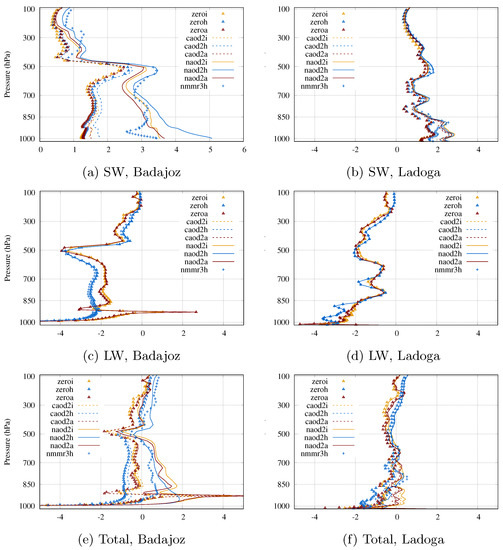
Figure 1.
Temperature tendencies due to radiation (K/day) at Badajoz (left column) and Ladoga (right column): SW tendency (a,b), LW tendency (c,d), total tendency (e,f). y-axis shows the pressure in hPa. Colored curves correspond to the experiments and are labeled in the legends according to Table 1. The last letter in the label name denotes the radiation scheme with i for IFSRADIA, h for HLRADIA and a for ACRANEB.
When aerosols are excluded (ZERO), when the original coefficients are used (HLRADIA with HSA) or when the climatological aerosol load is assumed (CAOD2) all schemes show similar SW heating rates at Badajoz (Figure 1a), with a maximum of approximately 2.5 K/day in the upper troposphere. The SW heating rate increases by 2 to 3 degrees/day in the lower troposphere, greatest in the case of HLRADIA, when an estimated n.r.t. aerosol load is included in terms of AOD550 (NAOD2 curves in Figure 1a). When the HLRADIA scheme is used we also see a smoother LW profile with more/less cooling in the lower/upper troposphere than when IFSRADIA or ACRANEB is used. This is most likely due to its simplified LW radiation parametrization (Figure 1c, see also Appendix A.2). The inclusion of aerosols makes little difference to the LW cooling rates regardless of the radiation scheme. The total temperature tendency due to radiation is determined by the sum of the SW and LW contributions (Figure 1e), which tend to balance each other. At Ladoga (Figure 1b,d,f) the differences between the schemes due to aerosols are smaller because of the smaller aerosol load and its different composition.
The radiation fluxes at the surface and at the TOA are shown in Table 2. All schemes give similar results when aerosols are excluded. The exception to this is LW fluxes in the case of HLRADIA. Outgoing LWUT (positive upwards) is larger and LWDS (positive downwards) is smaller for HLRADIA than for the other schemes. Large LWUT means that the net radiation (the sum of SWNET and LWNET) at the TOA, denoted as NETT in Table 2, is smaller when HLRADIA is used. An overestimation of the atmospheric LW absorption by HLRADIA was shown also in [28] in experiments where aerosols were excluded.
Table 2.
Radiative fluxes at the surface and top of atmosphere.
SWDS is smaller when climatological (CAOD2) or n.r.t. (NAOD2) AOD550 is included in the experiments. The reduction in SWDS, compared to that in the absence of aerosols, is largest for HLRADIA. SWUT decreases somewhat when IFSRADIA or ACRANEB are used with the small aerosol load over Ladoga but it increases when HLRADIA is used for the same case. Over Badajoz, where the load is larger and dominated by desert dust, all experiments show an increase in SWUT, again with the largest increase when HLRADIA is used. In HLRADIA SWNET is diagnosed from the SW heating profile, where, by default, scattering by aerosols does not have an influence. The diagnostic values shown in Table 2 are corrected so that about half of the SW radiation scattered by aerosol particles is added to SWNET at each model level. This uncertainty in the diagnostics means that SWUT and NETT by HLRADIA are not suitable for comparison to the other radiation schemes for cases where aerosols are included. The LW fluxes are less sensitive to aerosols for each of the radiation schemes.
Figure 1 and Table 2 also include results from the NMMR3 experiment done using HLRADIA with CAMS aerosol data and ECMWF optical properties (blue crosses in Figure 1). The SW and total heating rates (Figure 1, top and bottom rows) differ from the other results, in particular in the lower troposphere of the Badajoz case. Here the lower tropospheric SW heating (Figure 1a) decreases by approximately 2 K/day compared to NAOD2. The differences in LW heating rates are small. SWDS from HLRADIA is higher compared to NAOD2 both at Badajoz and Ladoga. At Badajoz, the LW fluxes are also affected (Table 2).
From here we continue with more detailed analysis of aerosol radiative transfer by comparing HLRADIA MMR-based experiments to HLRADIA AOD-based experiments.
4.2. HLRADIA Experiments over Lake Ladoga and in Badajoz
4.2.1. SW and LW Radiative Transfer
Total-column diagnostics of the aerosol radiative transfer over Badajoz and Ladoga are given in Table 3 for all of the experiments except ZERO and HSA where external aerosol data were not used. In terms of column-integrated AOD550, the largest aerosol load (0.544) was present in the NMMR3 and NMMR2 experiments over Badajoz, where there was a significant intrusion of desert dust aerosols. The new IOPs were used in these experiments. The lowest AOD550 at Badajoz (0.085, CAOD2) occurred when the AOD550 climatology and prescribed IOPs were used. The broadband SW optical depths (TAU-SW) are smaller than the AOD550 values in all experiments at both locations. The total-column MMR of all aerosols combined (TOTMMR) is shown in Table 3 for the MMR-related experiments. TOTMMR is not directly correlated with the optical depths of the aerosol mixture because the optical properties are specific to each aerosol species.
SW transmission (SWTRAN) was smallest over Badajoz (0.78) in the NMMR3 and NAOD2 experiments and largest (0.98) in CMMR2. The values of SWABS, the diagnostic vertically integrated SW absorption, are less than 10% of SWTRAN. The SW scattering by aerosols is given by 1 − SWTRAN − SWABS. The maximum scattering (0.16) occurred at Badajoz in the NMMR3 experiment. LW optical depths are typically at least an order of magnitude lower than the SW optical depths. The lowest value of LW transmission (LWTRAN) was 0.90 for the NMMR2 and NMMR3 experiments at Badajoz, where the largest LW absorption (LWABS, 0.08) and scattering (0.02) occurred.
The NMMR3 and NMMR2 experiments use the same n.r.t. MMR data, with the difference being how the aerosols are distributed vertically on model levels. This leads to different SWTRAN values, 0.78 for NMMR3 and 0.85 for NMMR2 at Badajoz. The reason is related to the vertical distribution of the different aerosol species and the resulting optical properties. We will analyze this in more detail in Section 4.2.4.
Next we consider the SWNET and LWNET profiles at Badajoz and Ladoga (Figure 2). At Badajoz the maximum difference in SWNET at the surface for the ZERO (no aerosol) experiment compared to NAOD2 is 170 W/m or 26%, which is almost the same as the difference between ZERO and NMMR3 (Figure 2a). This difference is also of the same order of magnitude as the maximum differences seen in 3D HARMONIE-AROME experiments [11] for the same case study. The NMMR3 and NAOD2 experiments which involve n.r.t. data show the smallest SWNET at Badajoz while those based on climatological aerosols (CMMR2D, CAOD2D) have the largest SWNET. SWNET for NMMR2 appears between the fluxes from the other n.r.t experiments and the climatological experiments. The maximum difference in SWNET between the NAOD2 and ZERO experiments over Ladoga is smaller, 50 W/m or 13% (Figure 2b). The value of SWNET that is closest to that of the ZERO experiment occurs in the NMMR3 experiment.
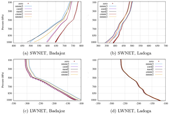
Figure 2.
Net HLRADIA radiative fluxes (Wm) for Badajoz (left) and Ladoga (right): SWNET (a,b) and LWNET (c,d). The curves correspond to the experiments in Table 1.
4.2.2. Broadband Optical Properties of the Aerosol Mixtures
Table 4 gives a summary of the vertically integrated broadband aerosol optical properties for the aerosol mixture used in the experiments. These were estimated from prescribed IOPs and atmospheric humidity profiles (see Section 2). Estimates of the scaled broadband SW and LW optical depths TAU-SW and TAU-LW, single-scattering albedos SSA-SW and SSA-LW and asymmetry factors ASY-SW and ASY-LW are shown. The single-scattering albedo is the ratio of scattering to total extinction and varies from 0 for a fully absorbing medium to 1 for a fully scattering medium. The asymmetry factor represents the fraction of forward scattering to total scattering. The optical depths are scaled by the factor 1 − SSA × (ASY) for the calculation of SW and LW absorption and scattering by aerosols within HLRADIA. TAU-SW and TAU-LW shown in Table 4 have been calculated from the vertically integrated SSA and ASY. Such estimates do not exactly represent the scaling that is done at each model level because of the non-linearity of the scaling factor.
For the Badajoz and Ladoga cases SSA-SW varied from 0.76 (NMMR3 for Ladoga) to 0.96 (CMMR2 for Badajoz). SSA-LW varied between 0.26 (Ladoga, NMMR2) and 0.39 (Ladoga, NAOD2). ASY-SW varied less and lay within the range 0.63–0.71. For ASY-LW the AOD550-based experiments showed values of around 0.2 while in the experiments based on MMR and new IOPs the values varied from 0.4 to 0.66. SSA and ASY differences between Badajoz and Ladoga reflect the different aerosol compositions at these locations and the different IOPs used in MMR-based and AOD-based experiments. We will come back to the optical properties of different aerosol species in Section 4.3.2.
4.2.3. Vertical Distributions
Figure 3 shows the vertical distribution of aerosol MMRs for the CMMR2, NMMR3 and NMMR2 experiments. The vertically integrated MMR input for CMMR2 is based on CAMS interim reanalysis 2003–2011 [7] as used by [26] while the column data for NMMR3 (unit kg/kg) was extracted from the CAMS n.r.t. database (see Appendix A.3 for the details of CAMS data). Input to NMMR2 was extracted from diagnostic output of NMMR3. The 2D aerosol MMRs (unit kg/m) were expanded vertically by using exponential profiles specific to the five aerosol types according to [9].
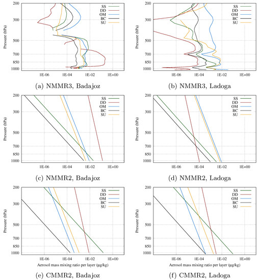
Figure 3.
MMR (g/kg) profiles for the (a,b) NMMR3 experiments, (c,d) NMMR2 and (e,f) CMMR2 over Badajoz (left) and Ladoga (right). y-axis shows pressure in hPa. Note the logarithmic scale on both axes.
Figure 3a,b show the different aerosol compositions over Badajoz and Ladoga. At Badajoz, a layer of desert dust is seen between 900 and 700 hPa where the maximum aerosol load reaches 0.1 g/kg on several of the lower tropospheric levels. The load of other species is at least one order of magnitude smaller. Over Ladoga, according to the CAMS n.r.t. dataset, OM and SU dominate but their concentrations only reach a maximum of 0.01 g/kg around 850 hPa. Figure 3c,d show the resulting aerosol concentration profiles when the n.r.t. data were first vertically integrated and then redistributed using the assumed exponential functions [9]. These profiles appear as straight lines on the log-log plots. The dominance of DD at Badajoz and OM and SU over Ladoga is clearly seen. Figure 3e,f show the expanded 2D climatological distributions, where the largest component is SS, followed by DD whose concentration is an order of magnitude smaller. The climatological SS and DD concentrations appear larger than the n.r.t. concentrations over Ladoga, and the SS concentration is also larger at Badajoz. For all other species, the climatological MMRs are smaller than the n.r.t. equivalents. Such compositions seem somewhat unrealistic especially for Ladoga, but may be explained by the coarse resolution of the input data, 3 × 3 degrees on a latitude-longitude grid, interpolated to the HARMONIE-AROME grid of 2.5 × 2.5 km. This means that every input value represents an area up to 1000 km that covers up to 160 fine-resolution grid points.
The composition of the aerosol mixture and IOPs of each aerosol type determine the broadband optical properties. The vertical distributions of aerosol species influence the profiles of TAU, SSA and ASY. The atmospheric humidity profile modifies the optical properties of hydrophilic aerosol species. The broadband SW and LW optical properties are illustrated in Figure 4 and Figure 5 for the Badajoz and Ladoga cases.
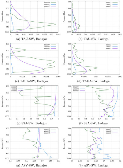
Figure 4.
Profiles of the aerosol SW optical properties for Badajoz (left) and Ladoga (right): TAU-SW (a,b), TAUA-SW (c,d), SSA-SW (e,f), ASY-SW (g,h). TAUA-SW denotes aerosol absorption optical depth, the rest of acronyms are explained in Table 4. Names in the curve legends correspond to the experiments in Table 1.

According to n.r.t. data (experiment NMMR3) TAU-SW reaches maximum values above the 850 hPa level both at Badajoz and over Ladoga (Figure 4a,b). When exponential profiles are used (experiment NMMR2), the distribution broadens in the vertical. The climatological distribution (CMMR2) shows smaller values especially over Badajoz. The influence of aerosol composition—hydrophobic desert dust dominates over Badajoz, hydrophilic sulfate and organic matter dominate over Ladoga—shows up in the NMMR2 profiles where the smooth exponential curve breaks for Ladoga due to vertical humidity variations. The absorption optical depth (TAUA-SW, Figure 4c,d) profiles are smoother because the strongest absorbing components are hydrophobic and the maxima are located higher in the atmosphere than the maxima of total TAU-SW. The SSA-SW (Figure 4e,f) and ASY-SW (Figure 4g,h) distributions show differences between experiments as well as vertical differences but the ranges of the variations is smaller.
4.2.4. An Example of Radiative Heating at Badajoz
Figure 6a shows the SW radiative heating for all the experiments included in Table 3. The heating suggested by the NMMR2 and NAOD2 experiments is most pronounced at the lowest model levels. In the 900–500 hPa layer the NMMR2 experiment shows less heating than NMMR3 and NAOD2. These differences are related to the SWTRAN differences shown in Table 3 and mentioned in Section 4.2.1. TAU-SW is slightly smaller in NMMR3 (0.465) than NMMR2 (0.471). However, the difference in SSA-SW values is greater: 0.78 for NMMR3 and 0.92 in NMMR2. This means that the aerosol mixture in NMMR3 is on average more absorbing than in NMMR2, where the average aerosol scattering is higher. The scaled TAU-SW values in Table 4 are larger (0.318) for NMMR3 than NMMR2 (0.272), which directly influences SWTRAN. Where does the difference in SSA-SW come from?
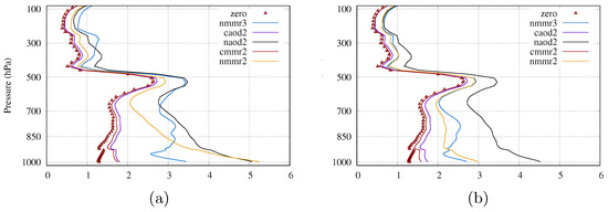
Figure 6.
Temperature tendencies due to SW radiation (K/day) at Badajoz: (a) all species included (b) black carbon excluded. y-axis shows pressure in hPa. Figure legends correspond to the experiments as given in Table 1.
The vertically integrated aerosol load in terms of MMR is the same in NMMR3 and NMMR2. For NMMR3 a 3D distribution of aerosol data obtained from CAMS is used (Figure 3a) while for NMMR2 exponential vertical profiles are assumed (Figure 3c). Differences in aerosol concentrations close to the surface and in the middle troposphere are seen. The differences in the upper troposphere are insignificant due to small aerosol loads there. The vertical distribution of the aerosol mass is reflected in the distribution of the optical properties. The SSA-SW values in NMMR3 above the dust layer are small, which indicates strong absorption (Figure 4e). This is confirmed by the fact that TAUA-SW has a second maximum at those levels (Figure 4c). Figure 3a shows that above 600 hPa the concentration of all aerosols other than DD is larger in NMMR3 than in NMMR2. Which of these causes the difference in SSA-SW that leads to the different SW heating rates in the middle troposphere?
Figure 6b shows what happens when BC is excluded from the experiments. Most notably, the heating profile of NMMR2 changes and becomes similar to NMMR3. The SW heating rates in NMMR2, NMMR3 and NAOD2 decrease somewhat. The second maximum in TAUA-SW, which is above the NMMR3 dust layer, disappears (not shown) and the SWTRAN values increase to 0.86 and 0.88 for NMMR3 and NMMR2 respectively, compared to 0.78 and 0.85. These differences are not large but the example shows the interaction between the distribution of different aerosol species and the optical properties. It suggests that it is important to account for such details when the aerosol loads of some species are substantial. In particular, the example shows a possible role of the strongly absorbing BC. In addition, from a methodology point of view the example demonstrates the power of single-column experiments as a tool for diagnosing and interpreting experiment results.
4.3. Species-Specific Sensitivity Tests
In this section, we focus on the results of the MMR and AOD series of experiments described in Table 1 with a focus on the impact of the different aerosol species. For the MMR series of experiments 11 bins of total-column MMR were combined to give the following 5 classes of aerosols: SS, DD, OM, BC and SU. The experiments were set up so that the resulting diagnostic AOD550 for each class was 0.5. The ratios within each class (e.g., between the three size bins of DD or hydrophilic and hydrophobic OM) were retained and the new IOPs were applied to the original 11 species when running the experiments. For the AOD experiments AOD550 = 0.5 was assigned to each of the Tegen aerosol categories: sea, desert, land, urban+sulfate. The default background values for stratospheric and tropospheric aerosols were still added, resulting in total AOD550 values of about 0.54 for each category. The default prescribed IOPs were used in the AOD series of experiments. The 5 aerosol classes in the MMR and AOD experiments are assumed to roughly correspond to one another.
4.3.1. SW and LW Radiative Transfer
The total-column diagnostics of the radiative transfer and broadband optical properties for each of the aerosol species are presented in Table 5 and Table 6 while Figure 7 shows the net radiative flux profiles. The SW transmission (SWTRAN = 0.56) was smallest for the case of BC in the MMR-BC experiment (Table 5). The transmission was larger (0.79) in the AOD-BC experiment where AOD550 input was combined with the old IOPs. This large difference is related to the optical properties. The values of SWABS diagnosed from MMR-BC suggest that the absorption capability of BC is at least an order of magnitude larger than that of the other species. Absorption by BC reduces SWTRAN even though the broadband TAU-SW is smaller (0.367) in the MMR-BC experiment than in AOD-BC (0.448). This is because the scaled TAU-SW (values presented in Table 6) is larger (0.365) in MMR-BC than in AOD-BC (0.309). In AOD-BC the scattering is 0.11 but in MMR-BC it is 0.06. The situation is the opposite for the more scattering SU or DD aerosols. For example, SWTRAN for DD is 0.84 in MMR-DD but 0.76 in AOD-DD, and in the latter SWABS is 5 times higher. This can also explain the differences between the NAOD2 and NMMR2 experiments at Badajoz, where the DD aerosol dominates (Figure 3) and SWTRAN is clearly larger in NMMR2 (0.85) than in NAOD2 (0.78) (Table 3).
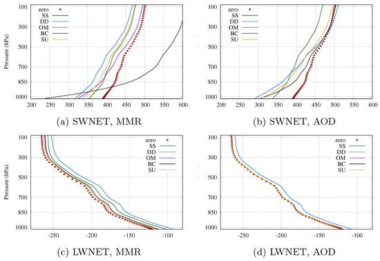
Figure 7.
Net radiative fluxes (Wm) for the MMR (left) and AOD550 (right) series of experiments: (a,b) SWNET and (c,d) LWNET. Figure legends correspond to the experiments as given in Table 1. SWD TOA = 779 Wm (conditions over Lake Ladoga).
The smallest LWTRAN values occurred in the MMR-DD (0.88) and AOD-DD (0.94) experiments because of the dominance of coarse particles. The results confirm that our parametrizations work as expected but also show that the MMR-based and AOD-based approaches lead to different LW transmission. Nevertheless, the impact of the difference on LW radiative fluxes is minor.
Figure 7 shows the LWNET and SWNET profiles for the MMR and AOD series of experiments. The maximum difference in SW fluxes compared to the ZERO aerosol experiment is somewhat smaller (ca. 100 Wm) in the AOD experiments than in the MMR experiments (ca. 200 Wm). The most striking feature of the MMR experiments is the strong impact of BC on SWNET, with the maximum impact occuring near the surface (Figure 7a). The impact is smaller in the AOD experiments (Figure 7b) although in both cases the vertically integrated AOD550 is approximately 0.5. In both cases, the 2D MMRs and AODs were distributed vertically using the same exponential functions. However, the IOPs and their wavelength and humidity dependencies are different, and this leads to different broadband optical properties and hence to different radiative fluxes. For SS and DD the different underlying assumptions concerning particle size distributions influence the differences seen in optical properties and radiative fluxes.
The differences between LW fluxes are smaller. The largest impact on the LWNET is due to DD, which is also the only species that appears different in the AOD experiments compared to the ZERO experiment (Figure 7d). In the MMR experiment series, the SS and BC cases result in slightly smaller upward (negative) LWNET on all model levels (Figure 7c).
4.3.2. Optical Properties of the Aerosol Species
Table 6 shows the vertically integrated SW and LW optical properties for the sensitivity experiments. The maximum TAU-SW occurred in the case of BC aerosol while the largest TAU-LW was related to DD. For the desert dust, TAU-LW is 30% of TAU-SW in MMR-DD but only 9% in the AOD-DD experiment. For sea salt, the relation of TAU-LW to TAU-SW was 0.49 in the MMR-SS experiment but only 0.03 in AOD-SS. Thus, for SS and DD the optical properties used in MMR experiments give more weight to LW impacts than AOD experiments. For all other species TAU-LW was an order of magnitude smaller than TAU-SW in the MMR experiments, and two orders of magnitude smaller in the AOD experiments. The MMR-BC SSA-SW and SSA-LW are the smallest (0.15 and 0.27) of all the experiments. This means that BC is highly absorbing and that the small amount of scattering is diffusive. The other species are mostly (forward) scattering in the SW part of the spectrum. All species, with the exception of SS in AOD-SS, are more absorbing than scattering in the LW (SSA-LW < 0.5 in Table 6).
Figure 8 shows the vertical distributions of the optical properties of each class of aerosol in a similar way to Figure 4 and Figure 5. The hydrophilic species—SS, OM and SU—show variations related to the vertical distribution of humidity while the hydrophobic DD and BC show smooth exponential distributions of TAU-SW and TAU-LW and constant values in the vertical for SSA and ASY, in the SW and LW parts of the spectrum. This explains the similar profiles at Badajoz and over Ladoga shown in Section 4.2.3. The highly absorbing BC and highly scattering DD show the largest values of TAUA-SW. As discussed earlier (Section 4.2.4), both of these species played a role in the experiments at Badajoz. In those experiments the differences between the n.r.t and prescribed exponential vertical distributions explain the difference in SWTRAN.
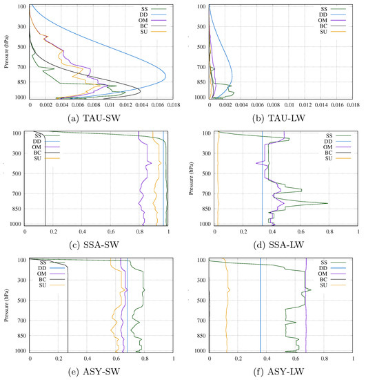
Figure 8.
Profiles of aerosol SW (left) and LW (right) optical properties for the five aerosol species in the MMR series of experiments: (a) TAU-SW, (b) TAU-LW, (c) SSA-SW, (d) SSA-LW, (e) ASY-SW and (f) ASY-LW. Acronyms are explained in Table 3 and Table 4. The figure legends correspond to the experiments according to Table 1.
5. Discussion
When the aerosol load is at a background or normal level, the aerosol concentration and optical property differences lead only to small differences in radiation fluxes and radiative heating. When the concentration of some aerosol species is higher than its background level, regionally or during pollution episodes, reliable 3D aerosol data become more important. To benefit from such data an accurate treatment of the optical properties of the different species becomes important.
The greatest differences were found between the experiments based on climatological AOD550 or MMR and those using n.r.t. data for the desert dust intrusion case over Badajoz. For example, SW transmission was 0.98 (0.97) when 2D climatological MMR (AOD550) was used but 0.78 when n.r.t. 3D MMR or 2D AOD550 was used. For the same case, LW transmission was 0.90–0.95 when n.r.t. aerosol data was used but 0.98–1.0 when climatological data were employed. In general, LW differences were smaller than SW differences. The value of 0.78 for SW transmission in the Badajoz experiment is in fact not very low. For example, based on satellite-based estimates [33] monthly mean values of less than 0.5 were recently reported over areas of India. Our example was that of desert dust whereas the aerosol composition over India is likely to be quite different.
Sensitivity studies using a total-column AOD550 = 0.5 for each aerosol species separately, demonstrated their respective impacts. To obtain AOD550 values of 0.5, 37 g of black carbon per square meter was required, whereas almost 1 g of sea salt results in the same AOD550. The SW transmission due to this amount of black carbon was 0.56 but 0.95 for sea salt, despite having the same AOD550 values. When AOD550 = 0.5 was used in conjunction with the old prescribed IOPs, the SW transmissivity increased to 0.79 for black carbon and decreased to 0.90 for sea salt. This demonstrates that it is important to account for the scattering and absorption properties of aerosol species, and not only to estimate the total AOD. An uncertainty in the estimated concentration of the species has different impacts: an inaccuracy of one g in the mass of black carbon may influence the radiative transfer more than a ten- or hundred-fold inaccuracy in the estimation of the mass of coarser particles.
The difference between the AOD and MMR sensitivity experiments is in how they handle optical properties. Both relied on vertically integrated AOD or MMR values that were distributed on model levels using the same species-specific exponential profiles. However, the optical properties depend not only on the vertical distribution of the aerosols but also on atmospheric humidity which varies significantly with elevation. Our new method of combining aerosol optical properties and mass distribution highlighted the sensitivity of radiative transfer to the vertical distribution of aerosol species. The introduction of new dependencies and interactions, even physically well-based, may increase the uncertainties of the calculations.
The single-column model framework allowed us to diagnose effects and interactions that cannot easily be detected using results of 3D model experiments. The main limitations of our study include the following which require further experimentation and developments:
- We have applied the simple HLRADIA scheme to determine the sensitivity of radiation fluxes and temperature tendencies to aerosol load and optical properties. HLRADIA was chosen for the practical reasons of availability and simplicity. Its known limitations, relating to the simplified treatment of atmospheric layers and the use of many empirical coefficients for the calculation of the SW and LW radiative transfer, must be taken into consideration. In particular, HLRADIA is unable to fully benefit from the 3D details of the aerosol optical properties suggested here. Also, as a broadband scheme, it is unable to use the spectral details of aerosol-radiation interactions that may become important in the LW range of the spectrum.
- In our MUSC experiments the surface temperature was intentionally kept constant by assuming a water/ice surface at the bottom of the atmospheric column. In reality, the local near-surface temperature changes related to aerosol impacts on radiation over land areas are assumed to arise from heating of the soil and not because of direct air temperature changes. However, MUSC is a less suitable tool for analyzing the evolution of temperature and other atmospheric variables over time because large-scale dynamical processes are ignored in the single-column framework.
- We have analyzed the impact of mineral dust in a Saharan dust intrusion case study. The impact of other aerosol species—sea salt, organic matter, black carbon and sulfates were only studied using artificial data under realistic atmospheric conditions. It would be interesting to study wildfire cases again, where organic matter, and possibly black carbon, impacts can be seen. Cases involving increased volcanic and anthropogenic emissions deserve further study. Stratospheric volcanic sulfates that are assumed to be a main factor in past climate cooling episodes at annual to decadal scales (see [34] and references therein) were not included. Stratospheric aerosols are poorly parametrized in limited-area NWP models and are not represented in the version of the CAMS dataset used in this study. However, volcanic emissions contribute to the tropospheric sulfate and dust loads in the CAMS dataset.
- We did not carry out tests using 3D climatological MMR data, that are available in the CAMS reanalysis dataset at high horizontal and vertical resolution and used in the ECMWF operational model [9]. We believe that for limited-area NWP models used for short-range weather forecasting, it is a higher priority to capture episodes of high aerosol load in real time than to address small systematic errors that may be related to the use of a coarse-resolution 2D aerosol climatology.
- Cloud–radiation–aerosol interactions were excluded from this study to focus on the direct radiative effects of aerosols. It is possible to estimate the first indirect effect of aerosols (Twomey effect) by parametrizing the cloud droplet number concentration (CDNC) using external aerosol data. Cloud particle effective size can be derived from CDNC and applied in the radiative transfer calculations. It is more complicated to take the impact of (hydrophilic) aerosols on the evolution of cloud droplets to precipitating particles into account. Single-column experiments can be used as a first step in formulating and testing the parametrizations.
To overcome the limitations of single-column studies, 3D HARMONIE-AROME experiments are required. Such experiments allow the study of aerosol impacts on weather parameters, and take dynamical processes and evolving surface interactions into account. They also enable quantification of aerosol-related uncertainties in weather forecasting. It is more useful to do such experiments using advanced radiation schemes which include radiative exchanges between atmospheric layers in cloudy and clear-sky cases. The results of 3D experiments should be compared to aerosol and radiation observations.
6. Conclusions and Outlook
In this study, we suggest improvements to the aerosol radiative transfer parametrizations in the ALADIN-HIRLAM NWP system. We have updated the calculation of aerosol optical properties in the HARMONIE-AROME configuration of the ALADIN-HIRLAM system. This was done using a combination of climatological 2D or n.r.t. 3D aerosol concentrations from CAMS and new pre-calculated IOPs from ECMWF. The resulting AODs, SSAs, ASYs for the aerosol mixture, at 16 LW and 14 SW wavelengths, were used to calculate broadband values of these optical parameters by applying spectral averaging over the SW (0.20–12.19 m) and LW parts (3.08–1000 m) of the spectrum.
These broadband optical properties were used by HLRADIA, the simplest radiation scheme available in HARMONIE-AROME, employing the approach in Enviro-HIRLAM [4,10]. The impact of the updated aerosol optical properties on the radiative fluxes and temperature tendencies was studied in single-column MUSC experiments. Both the aerosol concentrations, that originated from the CAMS dataset, and the atmospheric states were extracted from 3D HARMONIE-AROME experiments. For additional sensitivity studies, artificial 2D AOD550 and MMR data were prepared and used as input.
Using external 3D aerosol concentration data instead of climatological AOD550 data is beneficial for limited-area NWP models for several reasons. Until now, the treatment of aerosol inputs has usually been a part of the radiation schemes. We suggest that the 3D optical properties (AOD, SSA, ASY) of the aerosol mixture at each time-step of the model’s integration, taking the atmospheric humidity into account, be prepared outside of the radiation scheme. Using the actual optical properties as input enables radiative transfer calculations to be done applying any scheme without the need to treat the specific properties of individual aerosols. The possibility to choose between n.r.t. or climatological aerosol input data provides additional flexibility. Improved consistency between radiation and cloud parametrizations can be expected, in particular regarding the derivation and use of cloud particle effective sizes. In the future, n.r.t. data on the distribution of aerosols of different sizes and species could also be used in cloud microphysics parametrizations.
In this study, we have taken external aerosol data and IOPS as given, and focused on how to use these in a limited-area NWP model. Global integrated weather-chemistry models, with advanced data assimilation, presumably produce more reliable data than any regional integrated model. The CAMS global reanalysis data [7] are more detailed and more reliable than the older Tegen dataset [23]. However, the results from global weather-chemistry models contain uncertainties related to aerosol emission sources, assumptions used in the data assimilation, parametrizations of aerosol dynamics and the derivation of IOPs as discussed extensively in recent papers [7,9]. Additional inaccuracies arise from spatial and temporal interpolation of the coarse-resolution global aerosol data to the high-resolution limited-area NWP model grid.
Based on our results, we suggest the following steps to improve aerosol-related parametrizations in the ALADIN-HIRLAM NWP system:
- Include MMR-based 3D optical properties of the aerosol mixture for use by the IFSRADIA and ACRANEB radiation schemes to benefit from their more advanced SW and LW radiation transfer parametrizations compared to HLRADIA.
- Implement the method of importing n.r.t. high-resolution 3D CAMS MMR data to the ALADIN-HIRLAM system for use in operational weather forecasting. Investigate possible simplifications that would reduce the computational resource demand.
- Carry out extensive model-observation inter-comparisons for cases involving biomass burning, mineral dust intrusion, anthropogenic and volcanic emission to evaluate their impacts on local weather and radiation flux forecasts.
- Find optimal ways to use n.r.t. aerosol concentration data for derivation of cloud particle effective sizes, which are assumed to be the key parameters in the consistent treatment of aerosol-cloud-radiation interactions.
Author Contributions
L.R. introduced the renewed aerosol optical properties and climatological aerosol concentrations to the ALADIN-HIRLAM NWP system, designed and ran the MUSC experiments and prepared the original manuscript draft; E.G. participated in preparation and running of the MUSC experiments and edited the final text; D.M.P. introduced the n.r.t. CAMS aerosol to the ALADIN-HIRLAM system; K.P.N. is the author of the aerosol transfer code for HLRADIA, originally for Enviro-HIRLAM; V.T. was the first to introduce external climatological aerosol data and IOPs to the ALADIN-HIRLAM system. All authors contributed to the analysis of results, and writing and editing the manuscript. All authors have read and agreed to the published version of the manuscript.
Funding
V.T. acknowledges funding by the Estonian Research Council grant PSG202. L.R. thanks the Strategic Research Council at the Academy of Finland for funding through the BCDC Energy project (decisions 292854 and 314167).
Acknowledgments
We would like to thank Alessio Bozzo for the CAMS global aerosol MMR climatology and ECMWF aerosol optical properties datasets. The comments by the anonymous reviewers helped significantly to improve the presentation of our results. Support of the International HIRLAM-C Programme is also acknowledged.
Conflicts of Interest
The authors declare no conflict of interest.
Abbreviations
The most used abbreviations and symbols
| AOD | Aerosol Optical Depth |
| AOD550 | AOD at 550 nm |
| ASY | aerosol ASYmmetry parameter |
| ASY-LW | broadband LW ASY |
| ASY-SW | broadband SW ASY |
| BC | Black Carbon aerosol |
| CAMS | Copernicus Atmosphere Monitoring Service |
| DD | Desert Dust, mineral dust aerosol |
| IOP | aerosol Inherent Optical Properties |
| LW | LongWave, terrestrial radiation |
| LWD | downward LW flux |
| LWNET | net LW flux, the difference between LWD and LWU, positive towards the surface |
| LWU | upward LW flux |
| ME | Mass Extinction coefficient |
| MMR | Mass Mixing Ratio |
| n.r.t. | near-real time |
| NWP | Numerical Weather Prediction |
| OM | Organic Matter aerosol |
| SS | Sea Salt aerosol |
| SSA | aerosol Single-Scattering Albedo |
| SSA-LW | broadband LW SSA |
| SSA-SW | broadband SW SSA |
| SU | SUlfate aerosol |
| SW | ShortWave, solar radiation |
| SWD | downward SW flux |
| SWNET | net SW flux, the difference between SWD and SWU, positive towards the surface |
| SWU | upward SW flux |
| TAU | aerosol optical depth, the same as AOD |
| TAU-LW | broadband LW TAU |
| TAU-SW | broadband SW TAU |
| TAUA-SW | aerosol absorption optical depth |
| TOA | Top Of Atmosphere |
Appendix A. NWP Model and Aerosol Data
Appendix A.1. The Shared ALADIN-HIRLAM NWP System
The shared ALADIN-HIRLAM numerical weather prediction system [22], hereafter denoted the ALADIN-HIRLAM, is developed and maintained by those working in the ALADIN and HIRLAM NWP consortia. Many different configurations of the system are used by participating members, see Table A1 for abbreviations and references. The canonical configuration used by the authors of this paper is known as HARMONIE-AROME [29]. By default, HARMONIE-AROME includes two parametrizations of radiative transfer while a third scheme has been included in a development branch. Details on these radiation parametrizations are provided in Appendix A.2.
The single-column configuration of the ALADIN-HIRLAM called MUSC (Modèle Unifié, Simple Colonne), was used for the sensitivity tests presented in this paper. This 1D tool has primarily been developed by Météo France [30] but has a growing user and developer base in both HIRLAM and ALADIN countries. The tool was initially developed for validating and comparing physical parametrizations in the NWP system. In an NWP system the dynamical and physical processes are split into vertical and horizontal contributions. For physical processes, the horizontal contributions are neglected making it possible to isolate a column from the full model. Nevertheless, MUSC shares the same source code as the 3D model and is therefore always kept up-to-date with recent developments.
MUSC requires an initial state of the atmosphere, surface and physiographic information as input. Forcings are needed to determine the tendencies due to advection from neighboring columns. Both the initial state and atmospheric forcing can be extracted from the results of a full HARMONIE-AROME forecast for example. It is possible to provide a background state that the profile can relax towards during the time-integration. However, a profile can easily drift away from a realistic atmospheric state and there is no interaction with the large-scale flow which makes such a set-up unsuitable for real weather forecasting. MUSC is computationally very cheap and it is easy to replace parametrizations and to study problems by specifying forcings. This makes it a very useful tool for investigating model sensitivities. In this study, we use MUSC in diagnostic, rather than forecasting, mode where we extract the output from the first time-step of the model integration to avoid the issues just mentioned. In diagnostic mode atmospheric forcings are not needed.
Appendix A.2. Radiation Schemes in HARMONIE-AROME
In this section, we summarize the basic properties of three radiation schemes that are available within HARMONIE-AROME.
Appendix A.2.1. IFSRADIA
The scheme used by default is an old version of the European Centre for Medium-Range Weather Forecasts (ECMWF) radiation scheme from cycle 25R of their Integrated Forecasting System (IFS) [35] (Section 2), in this paper denoted as IFSRADIA. This scheme has 6 shortwave and 16 longwave spectral bands. The optical properties of clouds are determined from temperature, cloud cover, cloud liquid and ice content, and cloud particle effective radii; the latter are parametrized. Ozone and aerosol (AOD550) climatologies are used, and except for water vapor, which is a prognostic output variable, climatologies of other atmospheric gases are used. Overall, the scheme is computationally heavy and as a result is only called 4 to 5 times an hour during the forecast.
Appendix A.2.2. ACRANEB
The second scheme is a simpler, more computationally efficient, broadband scheme, called ACRANEB2 ([36,37], denoted ACRANEB in this paper). Versions of this scheme have been used in the ALADIN NWP model [22] since the 1990s. The optical properties of atmospheric gases, clouds, aerosols (AOD550) and the surface are derived from the data available within HARMONIE-AROME. ACRANEB includes an advanced treatment of LW interactions between the atmospheric layers resolved by the model. By default, cloud-radiation interactions are fully taken into accounted at each model time-step while the impact of atmospheric gases is calculated less frequently.
Appendix A.2.3. HLRADIA
The third scheme, included only in development versions of HARMONIE-AROME, is known as HLRADIA [28]. This scheme originates from the HIRLAM NWP model [38]. It is based on a pioneering study by [27], who suggested a quick and simple radiation scheme for mesoscale NWP models in which the SW and LW radiative transfer is parametrized by empirical fitting to detailed reference calculations. The radiative effects of atmospheric gases, ozone and aerosols are, by default, approximated using constant coefficients for the LW and SW intervals. This scheme is always called at every time-step of the forecast run. Because this scheme was used for all the sensitivity tests carried out in this study, further details about the parametrization are provided in the paragraph below.
SW and LW transmission and LW absorption are calculated for three atmospheric layers—a layer above the clouds, in the clouds themselves and below the clouds. Multiple cloud layers are treated as a single thick layer ignoring the clear-sky layers between them. For clear-sky cases the transmission/absorption is calculated for the entire atmospheric column. Diagnostic SWNET and LWNET at each model level are calculated for the model output. The fluxes are obtained by integrating the parametrized temperature tendencies from the surface up to the TOA and using SWNET and LWNET at the surface as boundary conditions.
In the SW part of the spectrum HLRADIA estimates the clear-sky flux from the TOA either to the cloud top or to the surface, taking the overlying atmospheric conditions into account. Atmospheric heating due to SW absorption by gases, aerosols and cloud particles is calculated at each model level from the TOA down to the surface. However, the absorption of the scattered radiation is not explicitly taken into account. The HLRADIA parametrization of LW heating assumes that each atmospheric level cools to space and interacts with the surface and the layer of clouds, if there. This means that the interactions between adjacent model levels are ignored. LW heating is calculated at each model level using the average above/in/below-cloud transmission and absorption.
The outgoing radiative fluxes (LWUT and SWUT) at the TOA were found earlier to be mostly overestimated by HLRADIA compared to reference results when aerosols were excluded. Absorption of SW radiation by atmospheric gases appeared to be underestimated and LW absorption overestimated [28]. This is due to the simplified treatment of atmospheric layers in HLRADIA and the use of many empirical coefficients to calculate the SW and LW radiative transfer.
These simplifications also influence the new aerosol radiative transfer parametrizations introduced to HLRADIA. Aerosol SW and LW transmission and LW absorption are calculated for three atmospheric layers—a layer above the clouds, in the clouds and below the clouds. Multiple cloud layers are treated as a single thick layer where the clear-sky layers in between are ignored. In cases without clouds, aerosol transmission and absorption are calculated for the entire atmospheric column.
The downwelling SW flux at the top of the cloud or at the surface is estimated by taking the aerosol transmission from the TOA to the model level in question into account. Only the SW absorption by aerosols is calculated in detail, level by level using the absorption optical depth from the TOA to each level. LW heating is calculated at each model level using the average above/in/below-cloud transmission and absorption. The averages are obtained by integrating the model level AOD, SSA and ASY in the column between the top and bottom of each of the three layers but from the TOA to the surface in the clear-sky conditions.
Appendix A.3. CAMS Mass Mixing Ratios (MMR) and ECMWF IOP Data
The 11 aerosol species [7,9] in the CAMS datasets describe the following 5 aerosol categories: sea salt (SS), mineral dust (DD), organic matter (OM), black carbon (BC) and sulfate (SU). Three size bins are used to describe the SS and DD aerosols. The bin limits for DD are 0.03, 0.55, 0.9 and 20 m, while for SS they are 0.03, 0.5, 5 and 20 m. For OM and BC hydrophilic and hydrophobic components are considered separately. In July 2019 CAMS was upgraded [39] to include three new aerosol fields representing nitrate and ammonium species. These new species have not been used in our experiments.
For this study, the monthly 2D CAMS MMR climatology [9,26] and 3D n.r.t. CAMS MMR data [8] were used. 11 aerosol species were used in each case. Input data (atmospheric and surface profiles) for the MUSC experiments were extracted from the output of corresponding 3D HARMONIE-AROME experiments as described below.
The global 2D MMR climatology and the corresponding IOPs of 11 aerosol species at 30 wavelengths were obtained from ECMWF courtesy of Alessio Bozzo (personal communication, December 2016). The monthly 2D MMR climatologies were introduced to a 3D HARMONIE-AROME experiment via the physiography (climate) generation step in the model. The 3-degree resolution data were interpolated bilinearly to the HARMONIE-AROME 2.5 km horizontal grid spacing. Once introduced to a HARMONIE-AROME experiment these aerosol data remain constant in time for the duration of the forecast.
3D n.r.t. CAMS aerosol data for needed dates were imported from CAMS +12 h forecast output via 3D HARMONIE-AROME experiments. The horizontal resolution of the CAMS global forecasting system is T511, which means that the Gaussian grid is truncated at wavenumber N = 256. At 45 degrees latitude the resolution is 0.35 degrees. In July 2019 the number of model levels in CAMS forecasts increased to 137 [39], the same number as in ECMWF’s high-resolution weather forecasting model. In this study, n.r.t. data with the previous vertical resolution of 60 levels was used. The n.r.t. CAMS MMR fields were interpolated to the HARMONIE-AROME grid of 2.5 km horizontal resolution and 65 levels in vertical. The data were introduced via the background fields of the 3D variational data assimilation and lateral boundary conditions. The model dynamics advects the fields during the forecast run.
Table A1.
Glossary of the ALADIN-HIRLAM system
Table A1.
Glossary of the ALADIN-HIRLAM system
| Acronym | Full Name | Purpose | Note |
|---|---|---|---|
| ALADIN-HIRLAM | Limited-area nonhydrostatic NWP system | [22] | |
| ALADIN | Aire Limitée Adaptation | Limited-area NWP model and consortium | Since 1990 |
| Dynamique Développement International | |||
| HIRLAM | High-Resolution Limited-Area Model | Limited-area NWP model and consortium | Since 1985 |
| AROME | Application of Research to Operations at Mesoscale | NWP configuration of ALADIN | [40] |
| HARMONIE | HIRLAM ALADIN Research for Mesoscale NWP in Europe | Configuration within ALADIN-HIRLAM | Since 2007 |
| HARMONIE-AROME | AROME configuration within HARMONIE | Bengtsson et al. [29] | |
| MUSC | Modèle Unifié, Simple Colonne | Single-column version of the system | Malardel et al. [30] |
Calculation of the aerosol IOPs, prepared for the ECMWF models and used for HARMONIE-AROME in this study, is described in detail by Bozzo et al. [9]. A log-normal size distribution of spherical particles is assumed for all the aerosol types to calculate the spectral ME, SSA and ASY for each aerosol type. For hydrophilic aerosol species hygroscopic growth is accounted for in the calculation of the optical properties. Organic matter represents a mixture of continental natural and anthropogenic aerosols. The properties of black carbon and sea salt originate from OPAC [24]. Sulfate includes industrial, volcanic and biogenic emissions. The optical properties of dust follow [41]. Figure A1 in [9] presents the optical properties of various aerosol types.
The 3D broadband optical properties (AOD, SSA, ASY) of the aerosol mixture were derived for HLRADIA using ECMWF IOPs. The basic data for 11 species, 30 wavelengths and 10 relative humidities were converted to a lookup table that is read at the initial step of each HARMONIE-AROME forecast. During each time-step of the forecast run, the relative humidity on the model’s 3D grid is used to select the needed values of ME, SSA and ASY. The run-time AODs of 11 species at 30 wavelengths are calculated at each grid point by combining the wavelength-dependent ME to the location and height-dependent MMR fields. The optical properties of the aerosol mixture at each wavelength are calculated as a sum of AODs over the 11 species and as the corresponding weighted averages of the SSA and ASY of each species. Finally, the weighted average over the 14 SW and 16 LW spectral bands defines the needed LW and SW broadband values of AOD, SSA and ASY of the aerosol mixture at each point of the 3D grid at each time-step. For the spectral weighting, the wavelength distribution of solar and terrestrial radiation was applied as in [4].
References
- Vogel, B.; Vogel, H.; Bäumer, D.; Bangert, M.; Lundgren, K.; Rinke, R.; Stanelle, T. The comprehensive model system COSMO-ART—Radiative impact of aerosol on the state of the atmosphere on the regional scale. Atmos. Chem. Phys. 2009, 9, 8661–8680. [Google Scholar] [CrossRef]
- Albani, S.; Mahowald, N.M.; Perry, A.T.; Scanza, R.A.; Zender, C.S.; Heavens, N.G.; Maggi, V.; Kok, J.F.; Otto-Bliesner, B.L. Improved dust representation in the Community Atmosphere Model. J. Adv. Model. Earth Syst. 2014, 6. [Google Scholar] [CrossRef]
- Baklanov, A.; Brunner, D.; Carmichael, G.; Flemming, J.; Freitas, S.; Gauss, M.; Hov, Ø.; Mathur, R.; Schlünzen, K.H.; Seigneur, C.; et al. Key Issues for Seamless Integrated Chemistry–Meteorology Modeling. Bull. Am. Meteorol. Soc. 2017, 98, 2285–2292. [Google Scholar] [CrossRef] [PubMed]
- Baklanov, A.; Smith Korsholm, U.; Nuterman, R.; Mahura, A.; Nielsen, K.P.; Sass, B.H.; Rasmussen, A.; Zakey, A.; Kaas, E.; Kurganskiy, A.; et al. Enviro-HIRLAM online integrated meteorology–chemistry modelling system: Strategy, methodology, developments and applications (v7.2). Geosci. Model Dev. 2017, 10, 2971–2999. [Google Scholar] [CrossRef]
- Flemming, J.; Peuch, V.-H.; Jones, L. Ten Years of Forecasting Atmospheric Composition at ECMWF, ECMWF Newsletter 152. 2017. Available online: https://www.ecmwf.int/en/newsletter/152/news/ ten-years-forecasting-atmospheric-composition-ecmwf (accessed on 1 January 2020).
- Yu, S.; Mathur, R.; Pleim, J.; Wong, D.; Gilliam, R.; Alapaty, K.; Zhao, C.; Liu, X. Aerosol indirect effect on the grid-scale clouds in the two-way coupled WRF–CMAQ: Model description, development, evaluation and regional analysis. Atmos. Chem. Phys. 2014, 14, 11247–11285. [Google Scholar] [CrossRef]
- Inness, A.; Ades, M.; Agustí-Panareda, A.; Barré, J.; Benedictow, A.; Blechschmidt, A.-M.; Dominguez, J.J.; Engelen, R.; Eskes, H.; Flemming, J.; et al. The CAMS reanalysis of atmospheric composition. Atmos. Chem. Phys. 2019, 19, 3515–3556. [Google Scholar] [CrossRef]
- Copernicus Atmosphere Monitoring Service (CAMS). 2019. Available online: https://atmosphere.copernicus.eu/data (accessed on 1 January 2020).
- Bozzo, A.; Benedetti, A.; Flemming, J.; Kipling, Z.; Rémy, S. An aerosol climatology for global models based on the tropospheric aerosol scheme in the Integrated Forecasting System of ECMWF. Geosci. Model Dev. Discuss. 2019. in review. [Google Scholar] [CrossRef]
- Gleeson, E.; Toll, V.; Nielsen, K.P.; Rontu, L.; Mašek, J. Effects of aerosols on clear-sky solar radiation in the ALADIN-HIRLAM NWP system. Atmos. Chem. Phys. 2016, 16, 5933–5948. [Google Scholar] [CrossRef]
- Rontu, L.; Pietikäinen, J.-P.; Martin Perez, D. Renewal of aerosol data for ALADIN-HIRLAM radiation parametrizations. Adv. Sci. Res. 2019, 16, 129–136. [Google Scholar] [CrossRef]
- Toll, V.; Reis, K.; Ots, R.; Kaasik, M.; Männik, A.; Prank, M.; Sofiev, M. SILAM and MACC reanalysis aerosol data used for simulating the aerosol direct radiative effect with the NWP model HARMONIE for summer 2010 wildfire case in Russia. Atmos. Environ. 2015, 121, 75–85. [Google Scholar] [CrossRef]
- Toll, V.; Gleeson, E.; Nielsen, K.P.; Mannik, A.; Mašek, J.; Rontu, L.; Post, P. Impacts of the direct radiative effect of aerosols in numerical weather prediction over Europe using the ALADIN-HIRLAM NWP system. Atmos. Res. 2016, 163–173. [Google Scholar] [CrossRef]
- Freitas, S. Evaluating Aerosols Impacts on Numerical Weathe Prediction: A WGNE/WMO Initiative. 2015. Available online: https://presentations.copernicus.org/EGU2015-7360_presentation.pdf (accessed on 12 January 2020).
- Poliukhov, A.A.; Chubarova, N.E.; Blinov, D.V.; Tarasova, T.A.; Makshtas, A.P.; Muskatel, H. Radiation Effects of Different Types of Aerosol in Eurasia According to Observations and Model Calculations. Russ. Meteorol. Hydrol. 2019, 44, 579–587. [Google Scholar] [CrossRef]
- Mulcahy, J.P.; Walters, D.N.; Bellouin, N.; Milton, S.F. Impacts of increasing the aerosol complexity in the Met Office global numerical weather prediction model. Atmos. Chem. Phys. 2014, 14, 4749–4778. [Google Scholar] [CrossRef]
- Rémy, S.; Kipling, Z.; Flemming, J.; Boucher, O.; Nabat, P.; Michou, M.; Bozzo, A.; Ades, M.; Huijnen, V.; Benedetti, A.; et al. Description and evaluation of the tropospheric aerosol scheme in the European Centre for Medium-Range Weather Forecasts (ECMWF) Integrated Forecasting System (IFS-AER, cycle 45R1). Geosci. Model Dev. 2019, 12, 4627–4659. [Google Scholar] [CrossRef]
- Fiedler, S.; Kinne, S.; Huang, W.T.K.; Räisänen, P.; O’Donnell, D.; Bellouin, N.; Stier, P.; Merikanto, J.; van Noije, T.; Makkonen, R.; et al. Anthropogenic aerosol forcing—Insights from multiple estimates from aerosol-climate models with reduced complexity. Atmos. Chem. Phys. 2019, 19, 6821–6841. [Google Scholar] [CrossRef]
- Bellouin, N.; Quaas, J.; Gryspeerdt, E.; Kinne, S.; Stier, P.; Watson-Parris, D.; Boucher, O.; Carslaw, K.S.; Christensen, M.; Daniau, A.L.; et al. Bounding global aerosol radiative forcing of climate change. Rev. Geophys. 2019. [Google Scholar] [CrossRef]
- Toll, V.; Christensen, M.; Quaas, J.; Bellouin, N. Weak average liquid-cloud-water response to anthropogenic aerosols. Nature 2019, 572, 51–55. [Google Scholar] [CrossRef]
- Baklanov, A.; Schlünzen, K.; Suppan, P.; Baldasano, J.; Brunner, D.; Aksoyoglu, S.; Carmichael, G.; Douros, J.; Flemming, J.; Forkel, R.; et al. Online coupled regional meteorology chemistry models in Europe: Current status and prospects. Atmos. Chem. Phys. 2014, 14, 317–398. [Google Scholar] [CrossRef]
- Termonia, P.; Fischer, C.; Bazile, E.; Bouyssel, F.; Brožková, R.; Bénard, P.; Bochenek, B.; Degrauwe, D.; Derkova, M.; El Khatib, R.; et al. The ALADIN System and its canonical model configurations AROME CY41T1 and ALARO CY40T1. Geosci. Model Dev. 2017, 11, 257–281. [Google Scholar] [CrossRef]
- Tegen, I.; Hoorig, P.; Chin, M.; Fung, I.; Jacob, D.; Penner, J. Contribution of different aerosol species to the global aerosol extinction optical thickness: Estimates from model results. J. Geophys. Res. 1997, 102, 23895–23915. [Google Scholar] [CrossRef]
- Hess, M.; Koepke, P.; Schult, I. Optical Properties of Aerosols and Clouds: The Software Package OPAC. Bull. Am. Meteorol. Soc. 1998, 79, 831–844. [Google Scholar] [CrossRef]
- Koepke, P.; Hess, M.; Schult, I.; Shettle, E.P. Global Aerosol Data Set; Report No. 243; Max-Planck-Institut für Meteorologie: Hamburg, Germany, 1997; ISSN 0937-1060. [Google Scholar]
- Bozzo, A.; Remy, S.; Benedetti, A.; Flemming, J.; Bechtold, P.; Rodwell, M.J.; Morcrette, J.-J. Implementation of a CAMS-Based Aerosol Climatology in the IFS; Technical Memorandum, 801; 2017; Available online: www.ecmwf.int/en/elibrary/17219-implementation-cams-based-aerosol-climatology-ifs (accessed on 1 January 2020).
- Savijärvi, H. Fast Radiation Parameterization Schemes for Mesoscale and Short-Range Forecast Models. J. Appl. Meteorol. 1990, 29, 437–447. [Google Scholar] [CrossRef]
- Rontu, L.; Gleeson, E.; Räisänen, P.; Nielsen, K.P.; Savijärvi, H.; Sass, B.H. The HIRLAM fast radiation scheme for mesoscale numerical weather prediction models. Adv. Sci. Res 2017, 14, 195–215. [Google Scholar] [CrossRef]
- Bengtsson, L.; Andrae, U.; Aspelien, T.; Batrak, Y.; Calvo, J.; de Rooy, W.; Gleeson, E.; Hansen-Sass, B.; Homleid, M.; Hortal, M.; et al. The HARMONIE-AROME model configuration in the ALADIN-HIRLAM NWP system. Mon. Weather Rev. 2017, 145, 1919–1935. [Google Scholar] [CrossRef]
- Malardel, S.; de Bruijn, C.; de Rooy, W. A Single Column Model of HARMONIE in KNMI Parametrization Testbed (CY33T1 version) (KNMI Report), De Bilt, The Netherlands. 2010. Available online: http://netfam.fmi.fi/muscwd11/docCY33.knmi.pdf (accessed on 6 December 2019).
- Tanré, D.; Geleyn, J.F.; Slingo, J. First results of the introduction of an advanced aerosol-radiation interaction in the ECMWF low resolution global model. In Aerosols and Their Climatic Effects; Gerber, H.E., Deepak, A., Eds.; A. Deepak Publishing: Hampton, VA, USA, 1984; pp. 133–177. [Google Scholar]
- Joseph, J.H.; Wiscombe, W.J.; Weinman, J.A. The Delta-Eddington Approximation for Radiative Flux Transfer. J. Atmos. Sci. 1976, 33, 2452–2459. [Google Scholar] [CrossRef]
- Lukose, L.; Dutta, D. Estimation of aerosol corrected surface solar irradiance at local incidence angle over different physiographic sub-divisions of India and adjoining areas using MODIS and SRTM data. J. Atmos. Ocean. Technol. 2019. [Google Scholar] [CrossRef]
- Rinne, J.; Alestalo, M. Volcanic impacts dominate bidecadal-multidecadal temperature variations during the late Holocene in Northern Fennoscandia. J. Geophys. Res. Atmos. 2019, 124, 11661–11671. [Google Scholar] [CrossRef]
- ECMWF. IFS Documentation, Chapter 2, 2015. Available online: http://www.ecmwf.int/sites/default/files/elibrary/2015/9211-part-iv-physical-processes.pdf (accessed on 1 January 2020).
- Geleyn, J.F.; Mašek, J.; Brožková, R.; Kuma, P.; Degrauwe, D.; Hello, G.; Pristov, N. Single interval longwave radiation scheme based on the net exchanged rate decomposition with bracketing. Q. J. R. Meteorol. Soc. 2017. [Google Scholar] [CrossRef]
- Mašek, J.; Geleyn, J.F.; Brožková, R.; Giot, O.; Achom, H.O.; Kuma, P. Single interval shortwave radiation scheme with parameterized optical saturation and spectral overlaps. Q. J. R. Meteorol. Soc. 2016, 142, 304–326. [Google Scholar] [CrossRef]
- Undén, P.; Rontu, L.; Arvinen, H.; Lynch, P.; Calvo, J.; Cats, G.; Cuxart, J.; Eerola, K.; Fortelius, C.; Garcia-Moya, J.A.; et al. The HIRLAM Version 5.0 Model. HIRLAM Documentation Manual (HIRLAM Scientific Documentation). 2002. Available online: hirlam.org (accessed on 1 January 2020).
- ECMWF News Release. Upgrade Improves Global Air Quality Forecasts. 2019. Available online: https://www.ecmwf.int/en/about/media-centre/news/2019/upgrade-improves-global-air-quality-forecasts (accessed on 1 January 2020).
- Seity, Y.; Brousseau, P.; Malardel, S.; Hello, G.; Bénard, P.; Bouttier, F.; Lac, C.; Masson, V. The AROME-France convective-scale operational model. Mon. Weather Rev. 2011, 139, 976–991. [Google Scholar] [CrossRef]
- Woodward, S. Modeling the atmospheric life cycle and radiative impact of mineral dust in the Hadley Centre climate model. J. Geophys. Res. 2001, 106, 18155–18166. [Google Scholar] [CrossRef]
© 2020 by the authors. Licensee MDPI, Basel, Switzerland. This article is an open access article distributed under the terms and conditions of the Creative Commons Attribution (CC BY) license (http://creativecommons.org/licenses/by/4.0/).