A Data-Driven Approach for Winter Precipitation Classification Using Weather Radar and NWP Data


Iowa Flood Center and IIHR—Hydroscience & Engineering, The University of Iowa, Iowa City, IA 52242, USA
Atmosphere 2020, 11(7), 701; https://doi.org/10.3390/atmos11070701
Submission received: 30 May 2020
/
Revised: 18 June 2020
/
Accepted: 24 June 2020
/
Published: 1 July 2020
(This article belongs to the Special Issue Radar Hydrology and QPE Uncertainties)
Abstract
:This study describes a framework that provides qualitative weather information on winter precipitation types using a data-driven approach. The framework incorporates the data retrieved from weather radars and the numerical weather prediction (NWP) model to account for relevant precipitation microphysics. To enable multimodel-based ensemble classification, we selected six supervised machine learning models: k-nearest neighbors, logistic regression, support vector machine, decision tree, random forest, and multi-layer perceptron. Our model training and cross-validation results based on Monte Carlo Simulation (MCS) showed that all the models performed better than our baseline method, which applies two thresholds (surface temperature and atmospheric layer thickness) for binary classification (i.e., rain/snow). Among all six models, random forest presented the best classification results for the basic classes (rain, freezing rain, and snow) and the further refinement of the snow classes (light, moderate, and heavy). Our model evaluation, which uses an independent dataset not associated with model development and learning, led to classification performance consistent with that from the MCS analysis. Based on the visual inspection of the classification maps generated for an individual radar domain, we confirmed the improved classification capability of the developed models (e.g., random forest) compared to the baseline one in representing both spatial variability and continuity.
1. Introduction
Precipitation is one of the most important variables in atmospheric and environmental sciences, including weather- and hydrology-related research. The estimation of rainfall (i.e., liquid phase precipitation) is becoming easier and more accurate thanks to advanced remote-sensing technology and the presence of reliable ground reference networks (e.g., [1,2]). On the other hand, quantifying amounts of solid and mixed precipitation remains challenging, as does identifying the many different types of precipitation (e.g., [3,4]) because of the difficulty of their reliable measurement. The information on this cold type of precipitation is important for infrastructure and facility management (e.g., air/ground traffic control and road closure) during the winter season in many regions (e.g., [5]). The conventional way of monitoring winter weather types (e.g., snow and freezing rain) has often relied on the dual-polarization capability of weather radars, which allows us to define hydrometeor types (e.g., [6]). These precipitation types obtained at the radar sampling locations aloft occasionally do not coincide with what is observed at the surface because of the possible phase transition along its falling path.
The Iowa Flood Center (IFC) has provided a real-time quantitative rainfall map for statewide streamflow prediction over the State of Iowa in the United States [7]. This radar-derived rainfall map is a composite of multiple radar datasets with a 5-min update cycle and an approximately 0.5 km resolution [8]. During the winter season, this map includes snow coverage information estimated using the numerical weather prediction (NWP) model data. This snow classification procedure does not incorporate radar observations to avoid the abovementioned disagreement between the ground and the radar sampling altitude; the rain/snow delineation applies two thresholds for surface temperature and critical thickness (e.g., [9,10]) retrieved from the High-Resolution Rapid Refresh (HRRR) model analysis (e.g., [11]). The real-time visualization of this map often reveals discontinuous snow regions split by a tile-shape border because the model’s resolution is coarser than the resolution of the rainfall map (i.e., 3 vs. 0.5 km). This discontinuous pattern continues until the model analysis is updated every hour.
In this study, we explore a data-driven approach to improve the discussed weakness of our current classification. We combine the data retrieved from radars and the NWP model to overcome the limitations of each radar- and NWP-only method and develop multiple classification models based on the supervised machine learning approach. Given the difficulty or uncertainty in classifying winter precipitation (e.g., [12,13]), our objective is to develop a framework that can deliver a multimodel-based classification ensemble or probabilistic classification product.
2. Data
In this study, we developed a data-driven model to classify winter precipitation for the entire State of Iowa in the United States. To ensure the model’s robustness and reliability, the modeling framework must include a variety of meteorological and environmental data resources retrieved from weather radars and an NWP model for multiple years. This dataset accounts for atmospheric conditions associated with precipitation microphysics (e.g., [14,15]). We used observed weather classes (e.g., rain, freezing rain, and snow) as reference information as recorded in the automated surface observing system (ASOS [16]) network. These records enable the supervised learning of our classification model and provide an opportunity to capture the dynamic features of winter precipitation processes because of the ASOS’s high observational frequency (e.g., 1 min).
2.1. ASOS Data
The ASOS is a joint effort initiated by the U.S. National Oceanic and Atmospheric Administration (NOAA), the Federal Aviation Administration (FAA), and the Department of Defense (DOD) to support weather forecasting research/activities and aviation operations. The ASOS network comprises over 900 stations across the United States, which provide a wide range of automated surface weather observations, such as temperature, precipitation, wind, pressure, visibility, and sky conditions [17]. In the study domain (i.e., Iowa) shown in Figure 1, there are 15 ASOS stations; we collected precipitation-type observations with a 1 min resolution from all 15 stations for selected events during a four-year period (2012–2015). As one of the ASOS stations is positioned within a range where no radar observation is available (i.e., “the cone of silence”), we excluded the data from the station (the one beside the KDVN radar in Figure 1) in our model development and validation. ASOS stations equipped with two sensors (one is for rain/snow identification, and the other is for freezing rain detection) for detecting weather types check the observed data and execute the precipitation identification (PI) algorithm every minute [17]. The PI result is categorized into three precipitation classes: (1) rain (−RA, RA, +RA), (2) freezing rain (−FZRA, FZRA), and (3) snow (−SN, SN, +SN). The negative (−) and positive (+) signs denote whether the strengths of the reported classes are “light” or “heavy”, respectively; no sign indicates a “moderate” state of precipitation.
2.2. Radar Data
We acquired the radar volume data (e.g., [18]) for four radars (see Figure 1) in the U.S. Weather Surveillance Radar-1988 Doppler (WSR-88D) network from Amazon’s big data archive (e.g., [19,20]). As illustrated in Figure 1, the four radars (KFSD in Sioux Falls, South Dakota; KDMX in Des Moines, Iowa; KDVN in Davenport, Iowa; and KOAX in Omaha, Nebraska) illuminate the Iowa domain with some overlaps and fully cover the ASOS locations. All four radars have provided polarimetric observations since their upgrade to dual-polarization (DP) in 2012 (KFSD, KDMX, and KDVN) and 2013 (KOAX). Their volume data contain three DP observables (differential reflectivity ZDR, copolar correlation coefficient ρHV, and differential phase φDP), including the conventional ones (horizontal reflectivity ZH, radial velocity, and spectrum width). To prepare the radar data for model development and evaluation, we assigned each individual radar to its closest ASOS station. The radar–ASOS pairs and the distances between them are listed in Table 1. We then retrieved the ZH, ZDR, and ρHV data observed at the base elevation angle (approximately 0.5°) for the corresponding spherical coordinates (e.g., 0.5° by 250 m in azimuth and range) of the ASOS stations from each assigned individual radar. The scanning intervals of WSR-88D are 4–5 min in a precipitation mode and 9–10 min for a clear air mode. The time of the radar observations for data retrieval was limited to a 1 min window from ASOS records. We did not include φDP observations in this procedure because φDP is a cumulative quantity along a radial direction and quite noisy except for in heavy rain cases. The relevance (or signature) of ZH, ZDR, and ρHV with different types of precipitation is well described in [1,3]. We note that there is no significant radar data quality control (except for a simple procedure using a ρHV threshold) included in the data retrieval to remove non-meteorological radar echoes because we selected obvious weather cases from the ASOS reports.
2.3. NWP Data
To define the weather conditions, we retrieved several atmospheric variables, which likely describe winter precipitation formation and development, from the Rapid Refresh (RAP) model analysis. The RAP is a continental-scale assimilation and model forecast system updated hourly and based on 13 and 20 km resolution horizontal grids [21]. For this study, we selected the 20 km horizontal grid data, assuming that the weather conditions do not sharply change within the 20 km grids collocated with the ASOS stations shown in Figure 1. The retrieved RAP variables for the corresponding ASOS record hours are the geopotential height at 1000, 850, and 700 mb; air temperature at the surface and 850 mb; and relative humidity at the surface. Because the critical thickness (e.g., [9,10]) is a typical indicator of snow-likely conditions, we derived two thickness layers between 1000–850 and 850–700 mb from the geopotential height at these pressure levels. The relative humidity combined with air temperature (e.g., wet bulb temperature) is another indicator that can account for the phase transition of precipitation and snow formation.
3. Methodology
In this section, we briefly introduce multiple models based on the supervised machine learning method for winter precipitation classification. Because of its efficiency and simplicity in model implementation, we used the Python “Scikit-Learn” library [22] to build multiple classification models. The six models selected for this study are k-nearest neighbors (kNN), logistic regression (LR), support vector machine (SVM), decision tree (DT), random forest (RF), and multi-layer perceptron (MLP). This section also outlines the model training and testing strategies for the objective evaluation of the models’ classification performance, depending on the refinement of precipitation classes and the different combinations of input features retrieved from the radar and NWP data.
3.1. Classification Models
One of the simplest classification algorithms is kNN, which does not require prior knowledge of the data (e.g., distribution). For a new data point, kNN attempts to define the point in the training dataset closest to the new point. The parameter k in the algorithm denotes how many of the closest neighbors to consider, and the algorithm makes a decision/prediction based on the majority class among the k nearest neighbors. While the kNN algorithm is often used as a baseline classification method, its performance (e.g., training time and prediction accuracy) tends to decrease as the training dataset becomes larger with an increasing number of features. In this study, we use a simple kNN model (i.e., k = 1) for training efficiency to test several different combinations of training features.
LR was named after the algorithm’s primary function, called a “logistic function”. This is also known as the “sigmoid function”, which allows predictive analysis based on the concept of probability (e.g., [23]). LR makes binary predictions by estimating the linear function parameters (i.e., slope and intercept) and transferring the linear estimates to the sigmoid function. For multiple class (e.g., n classes) identification, the algorithm analyzes n binary models, and for each of these, the classes are split into two groups, a specific class and all other classes. The algorithm then runs n binary classifiers for a new data point and makes its prediction by selecting a single class that yields the highest score.
SVM basically seeks a multi-dimensional hyperplane (e.g., decision boundary), which maximizes the margin/separation between two different classes. The hyperplane dimension is determined by the number of training data features. For instance, if there are two data features, the hyperplane is a line. As SVM is inherently a binary classifier [24], it is necessary to execute a procedure similar to the one in LR for multi-class identification. Support vectors defined as training points located near the border between classes determine the orientation and position of the hyperplane. To make a prediction, the algorithm measures the distances between a new data point and each support vector using a selected kernel function. The algorithm then makes its decision based on the measured distances and the weights of the support vectors. Because the kernel function is a key parameter in SVM, we tested several kernels (e.g., linear, sigmoid, polynomial, and radial basis functions) and selected the linear one for this study’s classification.
DT is a white-box type method, as opposed to a black-box model (e.g., neural network), which does not expose the model’s decision logic and rules. The DT algorithm begins by partitioning the tree in a recursive manner from the topmost decision node, known as the “root node”. The algorithm selects the best feature/attribute for splitting the data records at decision nodes and divides the records into smaller datasets (“branches”). It continues to the decision (“leaf”) at the end of the branch, where there is no more record to split. The algorithm applies a heuristic rule to decide the data-splitting criteria and assigns ranks to attributes (the best one is selected) based on attribute selection measures (ASM), such as the information gain, gain ratio, or Gini index (see, for example, [25]).
RF consists of a large collection of individual DTs, which result in an ensemble for a class decision. In other words, the individual DTs reach their own decisions, and the class with the highest occurrence becomes the model’s prediction. Given this basic concept, the most crucial factor in the determination of a model’s prediction performance is whether the model has a large number of (relatively) uncorrelated DTs. To avoid highly correlated trees in the forest, RF uses a random subset of all the provided features when building individual DTs, which makes the model stronger and more robust than a single DT by limiting model’s overfitting and increasing error caused by bias (e.g., [26,27]). In the RF model implementation, we set 100 trees for winter precipitation classification.
A perceptron is a simple binary classifier, which makes a prediction based on a linear transformation of an input feature vector using weights and a bias. On the other hand, MLP is a feedforward artificial neural network model that comprises at least three fully connected layers (i.e., input, hidden, and output layers) (e.g., [28]). MLP has two basic motions associated with model learning: (1) forward signals propagate from the input layer through the hidden layers and then reach a decision when the signals arrive at the output layers, and (2) the multitude of weights and biases are backpropagated and repeated until the decision error is minimized using a gradient-based optimization algorithm. While MLP provides a basis for deep learning, which facilitates a complex model structure to capture characteristics contained in large numbers of data, its training often takes longer than that of other models presented in this section. For the MLP model in this study, we set 100 hidden layers for training efficiency.
3.2. Model Training and Evaluation
Supervised model learning requires model input features (e.g., predictors) and target classes. The target classes used in this modeling procedure are rain, freezing rain, and snow (light, moderate, and heavy) as observed at the ASOS stations. While the ASOS records offer three rain classes (light, moderate, and heavy), we consolidate these into one simple class (i.e., rain) in this study. Quantitative rainfall information is widely available from radar-derived products (e.g., [8,29]), and there are fewer concerns about the qualitative discretization of rain classes. Light and moderate freezing rain are also combined into one class because there are fewer cases of freezing rain than other types during the data period. The input features used for model development are ZH, ZDR, ρHV, two critical thicknesses between 1000–850 and 850–700 mb (Thick1000–850 and Thick850–700), two air temperatures at the surface (Ts) and 850 mb (T850), and relative humidity (RHs) at the ASOS locations. To explore the classification capability of the selected models, we applied various model configurations using the different sets of classes and input features listed in Table 2. Our focus on selecting input features was to explore snow- and freezing rain-likely conditions using different combinations of the NWP variables (e.g., F1–F4). Since radar observations are requirements for generating a classification map with high space and time resolutions, we included them in the final feature set (F5).
We split the entire data period into a separate training period (2012–2013) and validation period (2014–2015), as shown in Figure 2. The sample sizes of each class for the training and validation periods are presented in Table 3. To assess the consistency and robustness of models’ performance, we conducted simultaneous model training and cross-validation using Monte Carlo simulations (MCS) as follows: (1) randomly select 75% of the entire training dataset and use the samples for model training, (2) evaluate model performance using the rest (25%) of the dataset, and (3) repeat the prior two steps 1000 times and calculate a success rate (represented as “score” in the resulting figures) for each repetition. This MCS approach allowed us to examine the distribution/variability of model predictions and compare the classification performance of all six models. We based our decision regarding the model input features on the MCS results achieved by testing the different sets of features (see Table 2) retrieved from the radar and NWP data. We then trained all the models again using the selected feature dataset for the entire training period and captured the models’ structure and parameters. We note that the input feature data listed in Table 2 required a scale transformation (e.g., standardization) before they could be used for model learning. This is because some learning algorithms (e.g., SVM and MLP) are often sensitive to inconsistency in the data scales among different input features, which causes a divergence of the algorithm cost function and leads to inaccurate predictions. We applied the final (trained) models and data transformation scheme saved from the model training step to the independent model evaluation using a new dataset for the validation period presented in Figure 2. For the purposes of visual comparison and assessment, we generated classification maps for two example weather cases using the developed models and the IFC’s threshold approach (hereafter referred to as the baseline method).
4. Results
4.1. Relationships between Classes and Features
The analysis begins with an inspection of the relationships between precipitation classes and the model input features retrieved from the radar and NWP data. This analysis examines how well the features (e.g., as explanatory variables) describe snow- or rain-likely conditions in the atmosphere and on the surface. The results from this analysis can provide useful guidance when selecting model input features and help us understand the classification performance derived from a specific set of input features. In Figure 3, we present the relationships between two explanatory variables arbitrarily selected from the NWP data and precipitation classes observed in the training period shown in Figure 2. Regarding radar variables (e.g., ZH–ZDR), [1,3] provide similar representation to Figure 3. Although there are many more possible combinations using all the input features, Figure 3 demonstrates a few representative combinations. We also note that this two-dimensional illustration has limited usefulness in scrutinizing multi-dimensional characteristics (dependence) between the explanatory and response variables. We hope that the machine learning models will address such characteristics. The critical thicknesses (Thick1000–850 and Thick850–700) and surface temperature (Ts) shown in Figure 3 are typical indicators commonly used to identify snow/rain (e.g., [9,10]). For example, the IFC applies two threshold values (i.e., 3 °C for Ts and 1310 m for Thick1000–850) to distinguish snow-likely regions and provides a real-time radar-derived rainfall map with snow area identification [8]. These two thresholds are presented in Figure 3 as red solid lines, and we use this baseline method as a benchmark when evaluating the machine learning models proposed in this study. As demonstrated in Figure 3, there is much overlap among the winter precipitation classes (cold rain, freezing rain, and snow), and warm rain is easier to discriminate. This implies that winter precipitation classification is quite challenging with such a threshold approach. However, the thresholds for Ts and Thick1000–850 presented in Figure 3 seem to be reasonable discriminators with an acceptable occurrence of classification errors (e.g., about 7% for the presented samples), given the simplicity of the method. Figure 3 also reveals that relative humidity (RHs) is another important factor in deciding rain/snow under certain conditions because cold and mixed (i.e., freezing) rain is not likely to form below 60% of RHs at lower surface temperatures.
4.2. Model Training and MCS
To decide the model input features, we tested several different sets of feature combinations (F1–F5) for a simpler precipitation class set (C1). The input feature and class sets are listed in Table 2. Figure 4 shows the MCS results for all the different feature sets and classification models described in Section 3.1. Each boxplot represents the distribution of classification scores (i.e., success rate) obtained from 1000 rounds of random resampling, and the scores were calculated with cross-validation using 25% of the entire training dataset. As shown in Figure 4, all the models perform better than the baseline method (indicated by a red solid line) except for some realizations with the F1 and F2 feature sets. We discovered that the classification score tends to increase as the models include more explanatory variables. This implies that the upper atmospheric layer information (i.e., Thick850–700 and T850) is a critical factor that leads to improved classification based on the sharp changes observed between the F2 and F3 distributions for all six models. The inclusion of radar observations yielded results that differ depending on the model learning schemes; most models result in similar or worse performance (e.g., F4 vs. F5), while RF shows slight improvement in terms of the median and interquartile range. Because RF seems to be the best model given the median (or the mean) and the variance of distribution (e.g., the width of the interquartile range) in Figure 4, we decided to select F5 for model input features. We also expect that the inclusion of radar variables supports frequent map updates (e.g., 4 to 5 min), which is not feasible with the NWP data only.
Using the final feature set (F5), we performed the MCS analysis once more for the class set C2 (see Table 2), which further refines snow classes from C1. As shown in Figure 5, the performance of all models for C2 significantly dropped when compared to that for C1. However, RF remains the best model, with a classification success rate of about 90%. Therefore, we examined the reason for the performance drop observed in Figure 5 and analyzed the misclassification rates of all five classes during the resampling procedure. For example, Figure 6a shows the distribution of RF’s misclassification rates with respect to each individual class. The sum of misclassification rates from all five classes reaches unity at each realization, and the distribution presented as a boxplot in Figure 6a indicates a collection of 1000-time simulation results. As presented in Figure 6a, MS was the most challenging one as defined by RF. We also confirmed that LS and MS contained most of the errors in MLP. We further tracked RF’s cases of misclassification for MS and present the results in Figure 6b, regarding the content of the errors derived from RF. In Figure 6b, we show that most MS cases were classified as LS, and the discrimination between LS and MS is the most challenging task in the refinement of snow classes.
While RF outperforms other models, it would be valuable to maintain all six models (because all models with the final feature set F5 performed better than the baseline method), which enables a multimodel-based ensemble or probabilistic approach. We finally trained all six models with the feature set F5 for the target precipitation classes C1 and C2 using the entire training dataset and saved the structure and parameters of the models. We added one more element to the model training stream to learn if sequential modeling, which performs the first classification for C1 and then refines the snow classes using C1’s result, can reduce errors compared to the direct classification for C2. Therefore, separate snow models were also trained for the classification of its three classes.
4.3. Model Evaluation
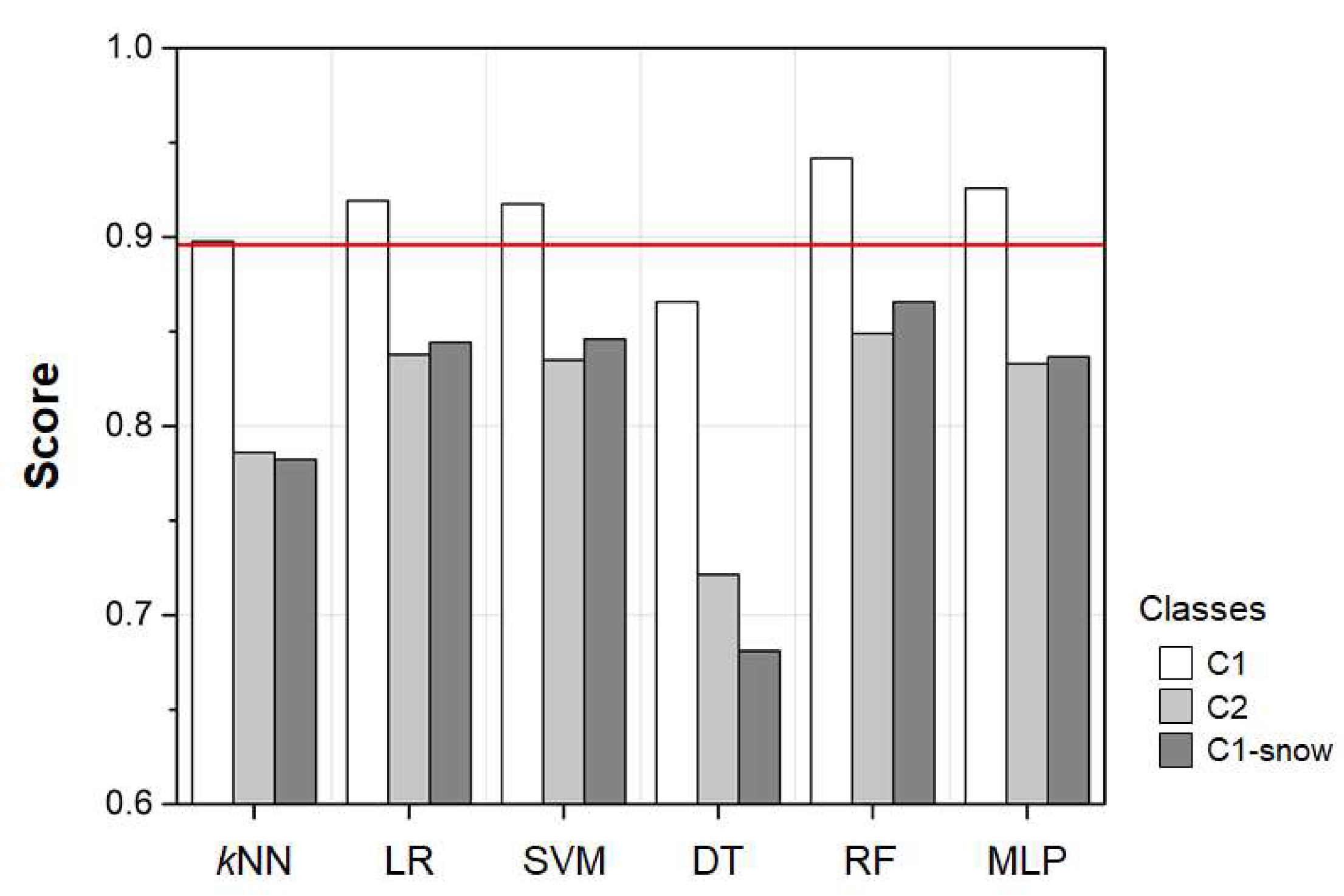
In this section, we evaluate the performance of all six models trained in the previous section using an independent dataset (see Figure 2) that was not used for model development and training. The evaluation results are illustrated in Figure 7 with respect to the target precipitation classes listed in Table 2. The results for C1 and C2 presented in Figure 7 show similar tendencies to those in Figure 5: (1) the performance drops from C1 to C2, and (2) RF performs the best for both C1 and C2. The label “C1-snow” in Figure 7 denotes the results of sequential modeling, which identifies the C1 classes first and then details the snow classes (light, moderate, and heavy) from SN in C1. As expected, the use of successive models (C1-snow) seems to improve the result slightly compared to the results from direct refinement (C2). The C1-snow approach tends to reduce the number of rain classes (e.g., FA and RA) that are erroneously classified into the refined snow classes. However, the performance difference between C2 and C1-snow does not seem significant, and most of the misclassification for both approaches appears between light and moderate snow, as shown in Figure 6. We also present the result of the baseline threshold method (a red solid line in Figure 7) for the validation dataset, which can be compared with that of C1 because the baseline method provides binary classification (rain/snow) only.
In Figure 8 and Figure 9, we applied the developed models to two well-known weather cases and generated classification maps for the KDVN radar domain. Figure 8 shows maps of radar reflectivity and precipitation classification (baseline and RF) for an event that occurred in May 2013 during the NASA’s field campaign, known as Iowa Flood Studies (IFloodS). The observed precipitation pattern, the presence of melting layer, and the precipitation types (e.g., phase) within the KDVN domain are described well in [30]. The baseline classification using two NWP parameters (Thick1000–850 and Ts) indicates that the coarse grid resolution of the NWP model generates an undesirable border between the precipitation classes. These discontinuous border and classification pattern persist until the model is updated, depending on the modeling cycle (e.g., hourly). On the other hand, the RF map using both the radar and NWP data better represents the spatial variability and provides an additional class (i.e., FR). In Figure 9, we present another case of widespread snow across the entire radar domain that occurred in March 2015. We confirmed the occurrence of both snow and freezing rain during this period based on the ASOS records and our personal experience (see Figure 2). While the RF map in Figure 8 shows three classes to be compared with the baseline method, Figure 9 illustrates the similarities and differences in the results produced by the different machine learning models (e.g., kNN, RF, and MLP) with five classes, as an example. As illustrated in Figure 9, RF seems to underestimate the coverage of freezing rain, whereas MLP defines a fairly extended area for the same class. Unfortunately, there is no reference information on this spatial coverage of freezing rain, and we speculate that the actual coverage pattern might be close to the one shown in the kNN map. Hopefully, we will be able to expand our training dataset and improve the models’ classification capabilities for freezing rain; we lacked sufficient cases of freezing rain in the development of our model.
5. Conclusions
This study proposes a framework for providing qualitative weather information on winter precipitation based on a data-driven approach using weather radar observations and NWP analysis. This framework enables the easy implementation of multiple classification models, which could lead to a multimodel-based ensemble or probability of occurrence for a precipitation class of interest. Using the widespread Python “Scikit-Learn” module [22], which supports a variety of machine learning studies, we constructed six supervised classification models: kNN, LR, SVM, DT, RF, and MLP. Although reference information on winter precipitation classes is uncommon, weather class observations [17] from two ASOS sensors allowed us to apply these supervised learning methods.
To determine which model input features properly describe winter precipitation processes, we tested several different feature combinations (Table 2) of the WSR-88D observations (ZH, ZDR, and ρHV) and the RAP analysis (Thick1000–850, Thick850–700, Ts, T850, and RHs) over Iowa in the United States. We performed random resampling, known as MCS, for each feature set by assigning 75% of the training samples for model learning and the rest for model cross-validation, and repeating these steps 1000 times. The MCS results for basic classification (rain, freezing rain, and snow) demonstrated that the model performance tends to improve with more feature information, particularly for the RF model, which showed the best classification performance of all six models. We also confirmed that based on the classification results from all the models for the selected feature set (F5), they outperform our current baseline method using two thresholds for Thick1000–850, and Ts. Although class refinement tends to decrease the accuracy of model classification (Figure 5), we found that the most frequent misclassification occurs between light and moderate snow, implying that the models’ basic classification is still valuable with high success rates.
The model evaluation using an independent dataset, which was not used for model learning, verified that the performance of the models remained within a range similar to that for the MCS results. We also made an effort to improve the performance decrease observed in class refinement by splitting the modeling procedure into two steps: basic classification and snow class refinement. This sequential modeling resulted in better classification than the direct refinement method, but the improvement did not seem significant. We also visually inspected the model-generated classification maps for well-known weather cases and found that the maps looked much more realistic than the one generated by the baseline method in representing spatial variability and eliminating discontinuous patterns arising from the coarse spatial resolution of the NWP data.
Based on this development, our goal is to implement the proposed models in our real-time operation [7] to improve the current binary classification (i.e., the baseline method). The inclusion of radar observations in the model input stream facilitates frequent map updates (e.g., every 5 min) with more precipitation classes and better representation of both spatial variability and continuity. The generation of a composite field map for a large area requires a data processing scheme to synchronize radar data (e.g., ZH, ZDR, and ρHV) or final classification maps generated at all different observation times from multiple radars. This can be readily resolved by calculating storm velocity vectors for each individual radar domain and projecting individual fields in a linear fashion with the vectors into synchronized space and time domains [31]. We note that the weather class information generated by this study is far from ready for use in quantitative applications (e.g., hydrologic prediction) because the estimation of snow density and snow-water equivalent is still challenging.
The reliability of data-driven models, particularly the supervised ones, depends on the accuracy of reference information. The sensors deployed in ASOS stations, which provide the class observations for supervised learning in this study, assign a certain portion of ice pellets into one of the rain categories (if they are accompanied by freezing rain, the sensor regards them as freezing rain) [17]. Ice crystals are regarded as no precipitation. Unfortunately, the degree and frequency of these uncertainties are unknown, and we hope to further investigate the effect of these factors on our classification using future cases. With the advantage of our data-driven framework, we will expand the model training dataset as the capacity of radar and NWP data grows and routinely train our models to make them more robust. While RF seems to perform better than other models with the current dataset, we hope that future data expansion and extensive model training will equalize the classification performance of all the models somewhat, leading to reliable ensemble production.
Funding
This research received no external funding and was supported by the Iowa Flood Center at the University of Iowa.
Acknowledgments
The author is grateful to Witold Krajewski for his insightful comments on the modeling and evaluation approach presented in the study. The author also thanks Kang-Pyo Lee from the Information Technology Services at the University of Iowa for providing his expertise on the machine learning models.
Conflicts of Interest
The author declares no conflict of interest.
References
- Ryzhkov, A.V.; Schuur, T.J.; Burgess, D.W.; Heinselman, P.L.; Giangrande, S.E.; Zrnic, D.S. The joint polarization experiment: Polarimetric rainfall measurements and hydrometeor classification. Bull. Am. Meteorol. Soc. 2005, 86, 809–824. [Google Scholar] [CrossRef] [Green Version]
- Kim, D.; Nelson, B.; Seo, D.-J. Characteristics of reprocessed hydrometeorological automated data system (HADS) hourly precipitation data. Weather Forecast. 2009, 24, 1287–1296. [Google Scholar] [CrossRef]
- Straka, J.M.; Zrnić, D.S.; Ryzhkov, A.V. Bulk hydrometeor classification and quantification using polarimetric radar data: Synthesis of relations. J. Appl. Meteorol. Clim. 2000, 39, 1341–1372. [Google Scholar] [CrossRef]
- Rasmussen, R.; Baker, B.; Kochendorfer, J.; Meyers, T.; Landolt, S.; Fischer, A.P.; Black, J.; Thériault, J.M.; Kucera, P.; Gochis, D.; et al. How well are we measuring snow: The NOAA/FAA/NCAR winter precipitation test bed. Bull. Am. Meteorol. Soc. 2012, 93, 811–829. [Google Scholar] [CrossRef] [Green Version]
- Black, A.W.; Mote, T.L. Characteristics of Winter-Precipitation-Related Transportation Fatalities in the United States. Weather Clim. Soc. 2015, 7, 133–145. [Google Scholar] [CrossRef]
- Park, H.; Ryzhkov, A.V.; Zrnić, D.S.; Kim, K.E. The hydrometeor classification algorithm for the polarimetric WSR-88D: Description and application to an MCS. Weather Forecast. 2009, 24, 730–748. [Google Scholar] [CrossRef]
- Krajewski, W.F.; Ceynar, D.; Demir, I.; Goska, R.; Kruger, A.; Langel, C.; Mantilla, R.; Niemeier, J.; Quintero, F.; Seo, B.-C.; et al. Real-time flood forecasting and information system for the State of Iowa. Bull. Am. Meteorol. Soc. 2017, 98, 539–554. [Google Scholar] [CrossRef]
- Seo, B.-C.; Krajewski, W.F. Statewide real-time quantitative precipitation estimation using weather radar and NWP model analysis: Algorithm description and product evaluation. Environ. Modell. Softw. 2020, (in press). [Google Scholar]
- Keeter, K.K.; Cline, J.W. The objective use of observed and forecast thickness values to predict precipitation type in North Carolina. Weather Forecast. 1991, 6, 456–469. [Google Scholar] [CrossRef] [Green Version]
- Heppner, P.O.G. Snow versus rain: Looking beyond the “magic” numbers. Weather Forecast. 1992, 7, 683–691. [Google Scholar] [CrossRef] [Green Version]
- Pinto, J.O.; Grim, J.A.; Steiner, M. Assessment of the high-resolution rapid refresh model’s ability to predict mesoscale convective systems using object-based evaluation. Weather Forecast. 2015, 30, 892–913. [Google Scholar] [CrossRef]
- Schuur, T.J.; Park, H.S.; Ryzhkov, A.V.; Reeves, H.D. Classification of precipitation types during transitional winter weather using the RUC model and polarimetric radar retrievals. J. Appl. Meteor. Climatol. 2012, 51, 763–779. [Google Scholar] [CrossRef]
- Thompson, E.; Rutledge, S.; Dolan, B.; Chandrasekar, V. A dual polarimetric radar hydrometeor classification algorithm for winter precipitation. J. Atmos. Ocean. Technol. 2014, 31, 1457–1481. [Google Scholar] [CrossRef] [Green Version]
- Thompson, G.; Rasmussen, R.M.; Manning, K. Explicit forecasts of winter precipitation using an improved bulk microphysics scheme. Part I: Description and sensitivity analysis. Mon. Weather Rev. 2004, 132, 519–542. [Google Scholar] [CrossRef] [Green Version]
- Zhang, G.; Luchs, S.; Ryzhkov, A.; Xue, M.; Ryzhkova, L.; Cao, Q. Winter precipitation microphysics characterized by polarimetric radar and video disdrometer observations in central Oklahoma. J. Appl. Meteorol. Climatol. 2011, 50, 1558–1570. [Google Scholar] [CrossRef] [Green Version]
- Clark, P. Automated surface observations, new challenges-new tools. In Proceedings of the 6th Conference on Aviation Weather Systems, Dallas, TX, USA, 15–20 January 1995; pp. 445–450. [Google Scholar]
- National Oceanic and Atmospheric Administration; Department of Defense; Federal Aviation Administration; United States Navy. Automated Surface Observing System (ASOS) User’s Guide, ASOS Program. 1998. Available online: https://www.weather.gov/media/asos/aum-toc.pdf (accessed on 30 May 2020).
- Kelleher, K.E.; Droegemeier, K.K.; Levit, J.J.; Sinclair, C.; Jahn, D.E.; Hill, S.D.; Mueller, L.; Qualley, G.; Crum, T.D.; Smith, S.D.; et al. A real-time delivery system for NEXRAD Level II data via the internet. Bull. Am. Meteorol. Soc. 2007, 88, 1045–1057. [Google Scholar] [CrossRef]
- Ansari, S.; Greco, S.D.; Kearns, E.; Brown, O.; Wilkins, S.; Ramamurthy, M.; Weber, J.; May, R.; Sundwall, J.; Layton, J.; et al. Unlocking the potential of NEXRAD data through NOAA’s big data partnership. Bull. Am. Meteorol. Soc. 2017, 99, 189–204. [Google Scholar] [CrossRef]
- Seo, B.-C.; Keem, M.; Hammond, R.; Demir, I.; Krajewski, W.F. A pilot infrastructure for searching rainfall metadata and generating rainfall product using the big data of NEXRAD. Environ. Modell. Softw. 2019, 117, 69–75. [Google Scholar] [CrossRef]
- Benjamin, S.G.; Weygandt, S.S.; Brown, J.M.; Hu, M.; Alexander, C.R.; Smirnova, T.G.; Olson, J.B.; James, E.P.; Dowell, D.C.; Grell, G.A.; et al. A North American hourly assimilation and model forecast cycle: The Rapid Refresh. Mon. Wea. Rev. 2016, 144, 1669–1694. [Google Scholar] [CrossRef]
- Pedregosa, F.; Varoquaux, G.; Gramfort, A.; Michel, V.; Thirion, B.; Grisel, O.; Blondel, M.; Prettenhofer, P.; Weiss, R.; Dubourg, V. Scikit-learn: Machine learning in Python. J. Mach. Learn. Res. 2011, 12, 2825–2830. [Google Scholar]
- Peng, C.Y.J.; Lee, K.L.; Ingersoll, G.M. An introduction to logistic regression analysis and reporting. J. Educ. Res. 2002, 96, 3–14. [Google Scholar] [CrossRef]
- Vapnik, V. Support vector machine. Mach. Learn. 1995, 20, 273–297. [Google Scholar]
- Raileanu, L.E.; Stoffel, K. Theoretical comparison between the gini index and information gain criteria. Ann. Math. Artif. Intell. 2004, 41, 77–93. [Google Scholar] [CrossRef]
- Liaw, A.; Wiener, M. Classification and regression by random forest. R News 2002, 2, 18–22. [Google Scholar]
- Belgiu, M.; Drăguţ, L. Random forest in remote sensing: A review of applications and future directions. ISPRS J. Photogramm. Remote Sens. 2016, 114, 24–31. [Google Scholar] [CrossRef]
- Gardner, M.W.; Dorling, S.R. Artificial neural network: The multilayer perceptron: A review of applications in atmospheric sciences. Atmos. Environ. 1998, 32, 2627–2636. [Google Scholar] [CrossRef]
- Zhang, J.; Howard, K.; Langston, C.; Kaney, B.; Qi, Y.; Tang, L.; Grams, H.; Wang, Y.; Cocks, S.; Martinaitis, S.; et al. Multi-Radar Multi-Sensor (MRMS) quantitative precipitation estimation: Initial operating capabilities. Bull. Am. Meteorol. Soc. 2016, 97, 621–638. [Google Scholar] [CrossRef]
- Seo, B.-C.; Dolan, B.; Krajewski, W.F.; Rutledge, S.; Petersen, W. Comparison of single and dual polarization based rainfall estimates using NEXRAD data for the NASA iowa flood studies project. J. Hydrometeor. 2015, 16, 1658–1675. [Google Scholar] [CrossRef]
- Seo, B.-C.; Krajewski, W.F. Correcting temporal sampling error in radar-rainfall: Effect of advection parameters and rain storm characteristics on the correction accuracy. J. Hydrol. 2015, 531, 272–283. [Google Scholar] [CrossRef]
Figure 1.
The locations of radars and automated surface observing system (ASOS) stations in the study domain. The circular areas centered on each radar indicate the 230 km coverage of individual radars.
Figure 1.
The locations of radars and automated surface observing system (ASOS) stations in the study domain. The circular areas centered on each radar indicate the 230 km coverage of individual radars.

Figure 2.
Data periods and precipitation events used for (a) model training and Monte Carlo Simulation (MCS) analysis and (b) independent model evaluation.
Figure 2.
Data periods and precipitation events used for (a) model training and Monte Carlo Simulation (MCS) analysis and (b) independent model evaluation.

Figure 3.
Precipitation classes characterized by the environmental variables retrieved from the numerical weather prediction (NWP) data. The precipitation classes (rain, freezing rain, and snow) were observed at the ground using the ASOS stations in Iowa. The red solid lines indicate the thresholds for surface temperature and critical thickness (1000–850 mb) in the baseline method.

Figure 4.
MCS results for the different combinations (F1–F5) of model input features with respect to the classification models. The MCS analysis was performed for the basic precipitation classes (C1). The boxplot describes the distribution of the classification success rate achieved from 1000 realizations. The baseline method indicated by the red solid line was estimated using the two thresholds for critical thickness and surface temperature shown in Figure 3.

Figure 5.
The comparison of MCS results for basic precipitation classes (C1) and further refinement of snow classes (C2). The feature set F5 was used for this analysis.
Figure 5.
The comparison of MCS results for basic precipitation classes (C1) and further refinement of snow classes (C2). The feature set F5 was used for this analysis.

Figure 6.
The distribution of (a) random forest (RF)’s misclassification rate with respect to each precipitation class. The classes presented in (b) indicate RF’s misclassification for MS, which shows the highest misclassification rate in (a).
Figure 6.
The distribution of (a) random forest (RF)’s misclassification rate with respect to each precipitation class. The classes presented in (b) indicate RF’s misclassification for MS, which shows the highest misclassification rate in (a).

Figure 7.
The results of independent model evaluation regarding different class sets. The red solid line indicates the classification success rate of the baseline method.
Figure 7.
The results of independent model evaluation regarding different class sets. The red solid line indicates the classification success rate of the baseline method.

Figure 8.
Example maps of (a) base scan reflectivity, (b) classification by the baseline method, and (c) classification by RF. The circular lines centered on the radar site demarcate every 50 km within a 230 km radar domain. The radial lines are positioned with a 30° interval.
Figure 8.
Example maps of (a) base scan reflectivity, (b) classification by the baseline method, and (c) classification by RF. The circular lines centered on the radar site demarcate every 50 km within a 230 km radar domain. The radial lines are positioned with a 30° interval.

Figure 9.
Example classification maps generated from (a) kNN, (b) RF, and (c) MLP.


Table 1.
Radar–ASOS pairs for matching precipitation classes and model input features retrieved from the radar data. The closest ASOS station was assigned to each individual radar, and the numeric values in parenthesis indicate the distance (km) between them.
Table 1.
Radar–ASOS pairs for matching precipitation classes and model input features retrieved from the radar data. The closest ASOS station was assigned to each individual radar, and the numeric values in parenthesis indicate the distance (km) between them.
| Radar | The Number of ASOS Stations | ASOS Stations |
|---|---|---|
| KFSD | 2 | EST (161.1), SPW (131.9) |
| KDMX | 7 | ALO (142.2), AMW (30.2), DSM (22.5), LWD (122.9), MCW (161.8), MIW (78.9), OTM (126.9) |
| KDVN | 5 | BRL (102.7), CID (98.3), DBQ (87.9), DVN (0.6), IOW (78.0) |
| KOAX | 1 | SUX (119.0) |
Table 2.
Model target classes and input features for various model configurations.
| Class (C) | C1 | RA (rain), FR (freezing rain), and SN (snow) |
| C2 | RA, FR, LS (light snow), MS (moderate snow), and HS (heavy snow) | |
| Feature (F) | F1 | Thick1000–850 and Ts |
| F2 | Thick1000–850, Ts, and RHs | |
| F3 | Thick1000–850, Thick850–700, Ts, and T850 | |
| F4 | Thick1000–850, Thick850–700, Ts, T850, and RHs | |
| F5 | Thick1000–850, Thick850–700, Ts, T850, RHs, ZH, ZDR, and ρHV |
Table 3.
The sample size of precipitation classes for the training (2012–2013) and validation (2014–2015) periods.
Table 3.
The sample size of precipitation classes for the training (2012–2013) and validation (2014–2015) periods.
| Classes | RA | FR | LS | MS | HS | Total |
|---|---|---|---|---|---|---|
| Training | 408 | 68 | 956 | 107 | 14 | 1553 |
| Validation | 134 | 51 | 803 | 63 | 15 | 1066 |
© 2020 by the author. Licensee MDPI, Basel, Switzerland. This article is an open access article distributed under the terms and conditions of the Creative Commons Attribution (CC BY) license (http://creativecommons.org/licenses/by/4.0/).
Share and Cite
MDPI and ACS Style
Seo, B.-C. A Data-Driven Approach for Winter Precipitation Classification Using Weather Radar and NWP Data. Atmosphere 2020, 11, 701. https://doi.org/10.3390/atmos11070701
AMA Style
Seo B-C. A Data-Driven Approach for Winter Precipitation Classification Using Weather Radar and NWP Data. Atmosphere. 2020; 11(7):701. https://doi.org/10.3390/atmos11070701
Chicago/Turabian StyleSeo, Bong-Chul. 2020. "A Data-Driven Approach for Winter Precipitation Classification Using Weather Radar and NWP Data" Atmosphere 11, no. 7: 701. https://doi.org/10.3390/atmos11070701
Note that from the first issue of 2016, this journal uses article numbers instead of page numbers. See further details here.