General Method Based on Regressive Relationships to Parameterize the Three-Parameter Depth–Duration–Frequency Curve

Abstract

This paper aims to present simple regressive equations to estimate the parameters of the three-parameter depth–duration–frequency (DDF) curve (3p-DDF), which accurately expresses, for a preassigned return period, the relationship between the rainfall depth and the rainfall duration over large duration ranges, from below 1 h (i.e., tens of minutes) to above 1 h (up to 24 h). These equations are developed to relate their parameters to those of the two-parameter DDF curve (2p-DDF), which can be estimated more easily being based on more readily available data related to rainfall durations above 1 h. In the applications, the regressive equations are first calibrated using recent pluviographic data in northern Italy, Germany, and Sweden. Two validation steps are then carried out to test the equations in terms of estimated rainfall depths using the same data as those used in the calibration step and data of stations from other geographic areas, i.e., Sicily in southern Italy, and from the past century, respectively. The results obtained prove this methodology capable of providing reliable estimation of short-duration rainfalls with various return periods in the absence of measurements with fine temporal resolution.

1. Introduction

Knowledge of extreme rainfall events with short (sub-hourly) durations is critical for risk assessment of flood and rainfall-triggered hazards and for correct design of hydraulic infrastructures (e.g., urban drainage systems), particularly in catchments with a short response time.

Generally, the depths of rainfall events with a certain duration and probability of non-exceedance are obtained by applying extreme value analysis to the time series of rainfall data. Then, the depth–duration–frequency (DDF) curves are defined to estimate the depth of extreme rainfalls with different durations from those considered in frequency analysis. To this end, several analytical expressions [1,2] have been suggested for DDF curves throughout the past century, including the two-parameter power (2p-DDF) and three-parameter (3p-DDF) curves. Although the 2p-DDF is still used by practitioners, it can significantly overestimate the depth of short-duration rainfalls [3]. Furthermore, as the duration approaches zero, the estimation of intensity provided by the 2p-DDF tends to infinity. Alternatively, 3p-DDF curves perform very well at estimating both hourly and sub-hourly duration rainfall depths [4]. However, to obtain 3p-DDF curves for short durations, precipitation data with high temporal resolution (sub-hourly) are needed, but they are rarely available with a sufficient long recording period. Therefore, in many cases, the depth of short-duration rainfall events must be estimated by precipitation data with coarser temporal resolution (i.e., hourly).

In the literature, several strategies have been proposed to solve the problem mentioned above. Most of these strategies assume scale invariance of the rainfall process, which means that the statistical properties of extreme rainfall processes at different durations are related by a scale-changing operator [5]. For instance, the authors of [6] showed that the cumulative distribution function for the annual maximum series of mean rainfall intensity has a simple scaling property over the range from 30 min to 24 h. The authors of [7] investigated a network of rain gauges in Palermo city, Italy, and showed that the statistical properties of the rainfall series have a scaling property over the range of 10 min–24 h. The authors of [8] pointed out that a scaling regime holds for the range of 20–60 min for rainfall series from rain gauges over Sicily. However, the scale invariance assumption has sometimes been proven inconsistent [9].

More recently, the authors of [10] developed a regional hybrid methodology to assess sub-hourly annual rainfall maxima on the basis of a linear relationship between the scale exponents of 2p-DDF and 3p-DDF curves, derived from hourly and sub-hourly precipitation data, respectively. In their study, the relationship among the exponents was investigated only for stations within Campania region, Italy. Moreover, the correlation among the other parameters of the 3p-DDF and 2p-DDF was not considered.

The novel idea behind the current study is to find general regressive relationships among the parameters of the 3p-DDF, derived from precipitation data below and above 1 h, as well as the parameters of the 2p-DDF derived from precipitation data above 1 h, which are independent of the return period and geographic area. These relationships can be used to parameterize the 3p-DDF at sites where sub-hourly data are not available for their thorough parameterization. Hereinafter, the relationship among the parameters of the two DDF curves is obtained using precipitation data from three countries. Then, their validity is tested against rainfall time series of different geographic areas and recording periods from those used for calibration. An innovative procedure is then proposed in the present paper to estimate the depth of sub-hourly extreme rainfall events starting from hourly precipitation data which can be directly applied to various geographic areas.

2. Materials and Methods

The methodology adopted to construct relationships for the estimation of 3p-DDF curve parameters as a function of 2p-DDF curve parameters is described in the flowchart of Figure 1. In the subsequent sections, the rainfall data are first described, followed by the various methodological elements.

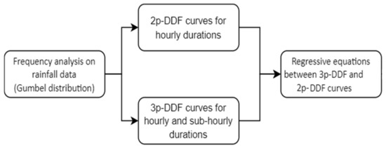
Figure 1. Flowchart of the methodology adopted.

2.1. Rainfall Data

The rainfall data used in this study were divided into two datasets (as shown in Table 1):

Table 1. Main characteristics of rain gauge stations used in this study.

Type of Data	Country	Location	Recording Period [Years]	Time Interval [min]	Maximum Recorded Rainfall [mm]
Dataset I	Italy	Pavia SS 35	2005–2019	10	20
	Italy	Bergamo	2004–2019	10	35
	Italy	Canevino	2008–2021	10	14
	Italy	Varzi	2004–2021	10	17
	Italy	Azzone	2004–2021	10	24
	Italy	Voghera	2004–2021	10	21
	Italy	Castello d’Agogna	2004–2021	10	25
	Italy	Varzi	2003–2018	10	20
	Italy	Cavenago d’Adda	2004–2021	10	24
	Italy	Monzambano	2005–2021	10	20
	Italy	Livigno	2005–2021	10	24
	Italy	Crema	2004–2021	10	22
	Italy	Santa Margherita di Staffora Casanova	2005–2021	10	19.8
	Sweden	Helsingborg	1996–2021	15	14
	Sweden	Hallands Väderö	1996–2021	15	15
	Sweden	Öland	1996–2021	15	16
	Sweden	Västmarkum	1996–2021	15	21.2
	Sweden	Film	2002–2021	15	20
	Sweden	Bjuröklubb	1996–2021	15	14
	Sweden	Pite-Rönnskär	1996–2021	15	11
	Sweden	Paharova	1996–2021	15	16
	Sweden	Ylinenjärvi	1996–2021	15	19
	Sweden	Ritsem	1998–2021	15	16
	Sweden	Gällivare	1996–2021	15	13
	Sweden	Latnivaara	1996–2021	15	29
	Sweden	Parkalompolo	1996–2021	15	11
	Sweden	Naimakka	1996–2021	15	14
	Germany	Großenkneten	2007–2021	10	17
	Germany	Ahrensfelde	2006–2021	10	19
	Germany	Albstadt-Badkap	2007–2021	10	19
	Germany	Alsfeld-Eifa	2005–2021	10	30
	Germany	Frauenwald	2005–2021	10	19
	Germany	Gelbelsee	2006–2021	10	11
	Germany	Walbeck	2005–2021	10	23
	Germany	Groß Kreutz	2006–2021	10	17
	Germany	Karstädt	2006–2021	10	20
	Germany	Kyritz	2005–2021	10	26
	Germany	Salzkotten	2007–2021	10	14
	Germany	Tribsees	2007–2021	10	19
	Germany	Lippoldsberg	2007–2021	10	20
Dataset II	Italy	Milano	1931–1970	15	34.5
	Italy	Erice	2003–2021	10	16
	Italy	Palermo	2003–2021	10	21.6
	Italy	Salemi	2003–2021	10	13.2

• Dataset I consisted of rainfall time series from 40 rain gauges with temporal resolution of 10–15 min, recording period ranging from 15 to 20 years, and maximum registered rainfall depth ranging from 11 to 35 mm, over Italy (13 stations in the northern area), Germany (13 stations), and Sweden (14 stations). This dataset was used to calibrate the regressive relationships.
• Dataset II consisted of rainfall data from four rain gauges. Three of them were stations from the region Sicily in southern Italy with a temporal resolution of 10 min and recording period of 19 years. The other one referred to the values of maximum annual rainfall depth with durations of 15, 30, 45, 60, 90, 120, 180, and 360 min, recorded by a rain gauge in Milan (Italy) over the years 1931–1970. These data were used for the validation of the relationships obtained using Dataset I.

2.2. Frequency Analysis on Rainfall Data and Depth–Duration–Frequency Curves

To derive the DDF curves for each rain gauge, first the rainfall quantiles with different durations had to be evaluated. For this purpose, the Gumbel probability distribution [11], which is one of the most widely used [12], was adopted. After removing outliers from the data and parameterizing the distribution, its suitability was verified with the Kolmogorov–Smirnov test at the 95% confidence level. According to the Gumbel distribution, the rainfall quantiles Q(T, t) for duration t and return period T can be expressed as:

$$Q\left(T,t\right)=u-\alpha \log \left[-log\left(\frac{T-1}{T}\right)\right],$$

(1)

where the distribution parameters u and α (for each duration t) were estimated by applying the following equations [13]:

$$\alpha =\frac{s \sqrt{6}}{\pi },$$

(2)

$$u=m-0.5772 \alpha ,$$

(3)

where m and s are the sample mean and standard deviation, respectively.

The considered return periods were 5, 10, and 15 years, i.e., typically adopted values for the design of urban drainage systems. The rainfall quantiles were computed for durations of 10, 20, 30, 40, and 60 min, or 15, 30, 45, and 60 min, for the stations with temporal resolution of 10 and 15 min, respectively, and for durations of 1, 3, 6, 12, and 24 h.

2.3. Depth–Duration–Frequency Curves

After obtaining the quantiles for each station, as well as the duration and return period as explained in Section 2.2, the 2p-DDF and 3p-DDF curves were obtained by fitting the quantiles with relationships expressing rainfall depth as a function of duration for each return period considered.

The 2p-DDF curve can be expressed as follows:

$$h\left(t\right)=a t^n,$$

(4)

where h(t) is the rainfall depth in mm, and t is duration in h. The optimized values for parameters a and n were estimated by applying the least squares method on the log–log plane of rainfall quantiles and duration (1, 3, 6, 12, and 24 h).

The 3p-DDF curve can be expressed as follows:

$$h\left(t\right)=\frac{a^{\prime }t}{{\left(t+c^{\prime }\right)}^{b^{\prime }}},$$

(5)

where, for any given value of the c′, Equation (5) becomes linear on the log–log plane, and a′ and b′ can be estimated using the least squares method. Therefore, an optimization was performed (using the fminsearch tool in MATLAB^®) on the value of c′ to maximize the coefficient of determination obtained in the least squares method. The 3p-DDF curves were estimated considering, at the same time, rainfalls with durations below and above 1 h.

2.4. Regressive Equations for the Parameters of DDF Curves

After obtaining the 3p-DDF and 2p-DDF curves for each rain gauge and return period, the relationship between parameters a and n and parameters a′, b′, and c′ was investigated. Since, from a mathematical point of view, h(t) is linearly dependent on a′ (in 3p-DDF curves) and a (in 2p-DDF curves), and since b’ and n are both exponents, the following kinds of relationship were explored:

$$a^{\prime }=f\left(a\right),$$

(6)

$$b^{\prime }=f\left(n\right).$$

(7)

Furthermore, since both the 3p-DDF and the 2p-DDF curves accurately estimate rainfall depth at long durations [4], a relationship was derived for the estimation of c′ for any t ≥ 1 h by enforcing the equality between Equations (4) and (5):

$$a t^n=\frac{a^{\prime }t}{{\left(t+c^{\prime }\right)}^{b^{\prime }}} \to {c^{\prime }}_{\left(t\right)}={\left(\frac{a^{\prime }}{a t^{n-1}}\right)}^{\frac{1}{b^{\prime }}}-t,$$

(8)

from which it follows that $c^{\prime }=f\left(a,n,a^{\prime },b^{\prime },t\right)$.

3. Results

The proposed methodology for deriving regressive equations among the parameters of the 3p-DDF and 2p-DDF curves was first applied (Section 3.1) and then validated (Section 3.2).

3.1. Calibration of Regressive Equations

After deriving the 3p-DDF and 2p-DDF curves for Dataset I, the relationships among their parameters (Equations (6) and (7)) were investigated. To measure the strength of association between two parameters, Spearman’s correlation (ρ) [14] was calculated as described in Equation (9).

$$\rho =1-\frac{6\sum d_i^2}{N\left(N^2-1\right)},$$

(9)

where d_i is the difference between the ranks of parameters, and N is equal to the number of rain gauges (40) multiplied by the number of return periods considered (three).

Notably, Figure 2 shows the values of parameter of a′ (3p-DDF) as a function of parameter a (2p-DDF) for all rain gauges in Dataset I, where the symbols dot, triangle, and star stand for return periods of 5, 10, and 15 years, respectively. As can be observed, there was a strong positive linear relationship between the two parameters (with ρ = 0.99), for which it was possible to derive the following regressive equation (with coefficient of determination R² = 0.99):

$$a^{\prime }=1.13 a-1.26.$$

(10)

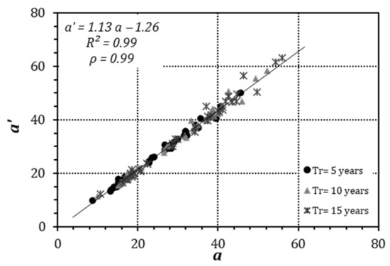
Figure 2. Regressive equation for the coefficients a′ (3p-DDF) and a (2p-DDF).

Figure 3 reports the relationship between the parameter b′ (3p-DDF) and the parameter n (2p-DDF) for all rain gauges and return periods. It can be noticed that the two parameters follow a negative linear trend (with ρ = −0.98), for which it was possible to derive the following regressive equation (with coefficient of determination R² = 0.98):

$$b^{\prime }=-1.13 n+1.05.$$

(11)

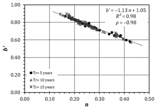
Figure 3. Regressive equation for parameters b′ (3p-DDF) and n (2p-DDF).

For the estimation of c′, Equation (8) was calculated for any t ≥ 1 h. Results not reported in this paper showed that the equation for t = 1 h performed well for all the stations and return periods, also leading to an even more simplified relationship:

$$c{\prime }_{\left(1\right)}={\left(\frac{a^{\prime }}{a }\right)}^{\frac{1}{b^{\prime }}}-1,$$

(12)

where subscript ₍₁₎ for c′ stands for t = 1 h. Moreover, by plotting the parameter c′ (obtained from the optimization) as a function of c′₍₁₎, as shown in Figure 4, it can be noticed that the two parameters follow a positive linear trend (with ρ = 0.92), for which it was possible to derive the following regressive equation (with coefficient of determination R² = 0.96):

$$c^{\prime }=1.21 c_{\left(1\right)}^{\prime }.$$

(13)

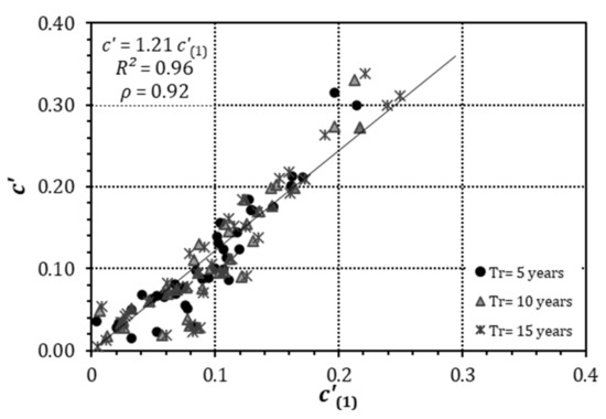
Figure 4. Regressive equation for the parameters c₍₁₎ and c′ (3p-DDF).

3.2. Validation of the Proposed Methodology

To validate the proposed methodology, Equations (10), (11) and (13) were verified for deriving new 3p-DDF curves (from here onward called estimated) to be tested against Dataset I, which was used for the calibration, and Dataset II, which was extracted from stations from different geographical region and recording periods. These two tests are described in Section 3.2.1 and Section 3.2.2, respectively. To quantify the error of DDF curves in estimating the rainfall depth in comparison with the Gumbel distribution, the standard error of estimate (S_e) and the index of agreement (d) [15] were calculated as described in Equations (14) and (15), respectively, for all types of DDF curve (2p-DDF, 3p-DDF, and 3p-DDF estimated).

$$S_e=\sqrt{{{\displaystyle \sum }}_{j=1}^N\frac{{\left(h_{DDF}-h^{*}\right)}^2}{N-1}},$$

(14)

$$d=1-\frac{{{\displaystyle \sum }}_{i=1}^N{\left(h_{DDF}-h^{*}\right)}^2}{{{\displaystyle \sum }}_{i=1}^N{\left[\left(h_{DDF}-\overline{h^{*}}\right)+\left(h^{*}-\overline{h^{*}}\right)\right]}^2},$$

(15)

where h_DFF and h^* are the rainfall depths calculated by DDF curves and Gumbel distribution, respectively, $\overline{h^{*}}$ is the mean value of h^*, and N is equal to the number of rain gauges (forty and four for the Dataset I and Dataset II, respectively) multiplied by the number of return periods considered (three).

3.2.1. Testing against the Data Used for Calibration

Rainfall depths obtained by Gumbel distributions (h^*) were compared with the rainfall depths (h_DFF) calculated using the following curves: 2p-DDF (star), 3p-DDF (grey dot), and 3p-DDF estimated with the proposed relationships (black dot), for each station of Dataset I. The comparison concerned each rain gauge and return period, as shown in Figure 5.

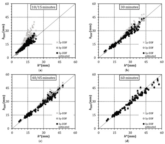
Figure 5. Comparison of rainfall depths from Gumbel distributions (h^*) and from 2p-DDF, 3p-DDF, and 3p-DDF estimated curves (h_DDF), for return period of 5, 10, and 15 years and duration of (a) 10/15 min, (b) 30 min, (c) 40/45 min, and (d) 60 min.

Notably, the comparisons between rainfall depths were performed for durations of 10, 30, 40, and 60 min, and 15, 30, 45, 60 min for stations with 10 and 15 min temporal resolution, respectively. From Figure 5a–d, the values for the 3p-DDF estimated curves overlapped well with the values of the optimal 3p-DDF curves, thus validating Equations (10), (11) and (13) derived for the estimation of the parameters a′, b′, and c′, respectively, in the absence of sub-hourly rainfall data. Furthermore, the rainfall depths calculated with both 3p-DDF curves were very close to the values from the Gumbel distributions. As expected, the rainfall depths from the 2p-DDF curves, instead, significantly overestimated them, especially for durations of 10/15 and 30 min. In Table 2, the standard error of estimate and index of agreement for the three types of DDF curves are reported. The 3p-DDF curves provided the best estimate of rainfall depths with durations from 10/15 to 60 min. The 3p-DDF estimated curves showed higher agreement and lower values of S_e than the 2p-DDF curves for durations of 10/15 min. For durations of 40/45 and 60 min, the S_e of the 2p-DDF curves became slightly lower than that of the 3p-DDF estimated curves (with a difference of less 1 mm). It is worth noting that the maximum difference between the S_e of the 3p-DDF and 3p-DDF estimated curves was roughly less than 1 mm for all the durations.

Table 2. Standard error of estimate (S_e) and index of agreement (d) of 2p-DDF, 3p-DDF, and 3p-DDF estimated curves in estimating the rainfall depth from Gumbel distribution.

		10/15 min	30 min	40/45 min	60 min
Se	2p-DDF	7.37	2.28	1.82	2.24
	3p-DDF	2.06	1.12	1.68	2.22
	3p-DDF estimated	2.21	2.20	2.33	2.51
d	2p-DDF	0.69	0.99	0.99	0.99
	3p-DDF	0.95	1.00	0.99	0.99
	3p-DDF estimated	0.94	0.98	0.99	0.99

3.2.2. Validation against the Data from Other Locations and Past Century

The same analysis as in Section 3.2.1 was carried out for three Italian rain gauges in Sicily (Erice, Palermo, and Salemi) and one in Lombardy (Milan) (called Dataset II in Table 1), with the aim of validating the proposed regressive equations for rainfall data different from those used for calibration. Notably, rainfall data from the region Sicily had a temporal resolution of 10 min and recording period of 19 years (from 2003 to 2021). Those for the Milan station, instead, had a temporal resolution of 15 min and recording period of 40 years (from 1931 to 1970).

The rainfall depths (h*) obtained with the Gumbel distributions were compared with the rainfall depths (h_DFF) calculated using the 2p-DDF (star), 3p-DDF (grey dot), and 3p-DDF estimated (black dot) curves for each rain gauge and 5, 10, and 15 year return periods, as shown in Figure 6, where the values for Sicily and Milan stations are separated by dashed lines. The comparisons across rainfall depths were performed for durations of 10, 30, 40, and 60 min, and 15, 30, 45, 60 min, for stations with temporal resolution of 10 and 15 min, respectively.

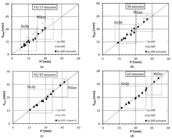
Figure 6. Comparison of rainfall depths from Gumbel distributions (h^*) and from 2p-DDF, 3p-DDF, and 3p-DDF estimated curves (h_DDF), for rain gauges in Sicily and Milan, with return periods of 5, 10 and 15 years and durations of (a) 10/15 min, (b) 30 min, (c) 40/45 min, and (d) 60 min.

As shown in Figure 6, also in this case, the 2p-DDF curves overestimated the values from the Gumbel distribution. On the other hand, the values for the 3p-DDF estimated curves were very similar to those of the optimal 3p-DDF curves, and both were very close to the values from the Gumbel distributions, thus validating Equations (10), (11) and (13) also for stations different from those used for the calibration.

The standard error of estimate and index of agreement for the four stations are shown in Table 3. The two 3p-DDF curves had quite similar values for index of agreement and S_e, which were significantly higher and lower than those of the 2p-DDF curves, respectively, especially for durations of 10/15 and 30 min, thus also proving the robustness and general validity of the proposed approach when applied on stations not used for the calibration of the equations.

Table 3. Standard error of estimate (S_e) and index of agreement (d) of 2p-DDF, 3p-DDF, and 3p-DDF estimated curves of stations in Sicily and Milan in estimating the rainfall depth from Gumbel distribution.

		10/15 min	30 min	40/45 min	60 min
Se	2p-DDF	7.35	3.88	1.73	1.28
	3p-DDF	1.25	1.43	1.03	1.26
	3p-DDF estimated	1.74	1.83	1.29	1.19
d	2p-DDF	0.85	0.96	0.99	1.00
	3p-DDF	0.99	0.99	1.00	1.00
	3p-DDF estimated	0.99	0.99	1.00	1.00

4. Discussion

The methodology proposed in this paper assumes that the parameters of the 2p-DDF and 3p-DDF curves are correlated from both mathematical and physical viewpoints, which was confirmed by the linear regressive equations derived for expressing their mutual relationship. When short-duration rainfall data are unavailable, these relationships can be used to obtain the 3p-DDF curves starting from the parameters of the 2p-DDF curves, which are calibrated with rainfall events with durations larger than or equal to 1 h. Ultimately, this enables estimation of short-duration rainfall depths at return periods ranging from 5 to 15 years, which are the typical values considered for the design of urban drainage systems. The validation tests, performed on data from different geographical regions and recording periods, highlighted the robustness and generalizability of the proposed methodology. The proposed methodology was found to have several advantages compared to those based on a scale invariance assumption, including the following:

• It does not require rainfall data with fine temporal resolution.
• It is applicable to various geographic areas.
• It can be used for different return periods.
• It is relatively straightforward to implement in practice.

It is worth noting that the value of the parameter c′ must be equal to or greater than zero [12]. Taking this constraint into account, and by substituting into Equation (12) the Equation (10) for parameter a’ (as shown in Equations (16) and (17)), it is possible to derive a limit for the applicability of the proposed method:

$${c^{\prime }}_{\left(1\right)}=\sqrt[b^{\prime }]{\frac{a^{\prime }}{a }}-1\ge 0 \to \frac{a^{\prime }}{a}\ge 1,$$

(16)

$$\frac{1.13 a-1.26}{a}\ge 1\to a\ge 9.69.$$

(17)

Equation (17) introduces a limit on the minimum value of a of the 2p-DDF curves below which the use of the proposed regressive equations leads to a negative value for c′. It should be noted that such a low value for the parameter a is uncommon. However, when this condition occurs, either the value of c′ can be set equal to zero, or the 2p-DDF curve can be used for the estimation of short-duration rainfalls depths.

5. Conclusions

In this study, simple regressive equations were presented for estimating the parameters of 3p-DDF curves, which can accurately estimate the depth of rainfall events with durations ranging from below 1 h (i.e., tens of minutes) to up to 24 h, for a preassigned return period. These equations were developed to relate the parameters of 3p-DDF curves to those of 2p-DDF curves, which are typically calibrated using rainfall data with the temporal resolution of 1 h. The regressive equations were derived using recent pluviographic data from northern Italy, Germany, and Sweden. The equations were then validated in terms of estimated rainfall depths with the same data as those used for the calibration, as well as with data from stations in other geographical areas and from the past century. The results obtained demonstrated the reliability of the proposed method in estimating short-duration rainfalls with different return periods and in different geographical areas, in the absence of rainfall data with fine temporal resolution, thus enabling the direct parameterization of the 3p-DDF. Potential future investigations will concern the assessment of the applicability and reliability of the proposed approach to stations from other geographic regions and for different return periods.

References

- Bernard, M.M. Formulas For Rainfall Intensities of Long Duration. Trans. Am. Soc. Civ. Eng. 1932, 96, 592–606. [Google Scholar] [CrossRef]
- Sherman, C.W. Frequency and Intensity of Excessive Rainfalls at Boston, Massachusetts. Trans. Am. Soc. Civ. Eng. 1931, 95, 951–960. [Google Scholar] [CrossRef]
- Di Baldassarre, G.; Brath, A.; Montanari, A. Reliability of Different Depth-Duration-Frequency Equations for Estimating Short-Duration Design Storms. Water Resour. Res. 2006, 42, W12501. [Google Scholar] [CrossRef]
- Garcia-Bartual, R.; Schneider, M. Estimating Maximum Expected Short-Duration Rainfall Intensities from Extreme Convective Storms. Phys. Chem. Earth Part B Hydrol. Ocean. Atmos. 2001, 26, 675–681. [Google Scholar] [CrossRef]
- Olsson, J.; Niemczynowicz, J.; Berndtsson, R. Fractal Analysis of High-Resolution Rainfall Time Series. J. Geophys. Res. 1993, 98, 23265. [Google Scholar] [CrossRef]
- Menabde, M.; Seed, A.; Pegram, G. A Simple Scaling Model for Extreme Rainfall. Water Resour. Res. 1999, 35, 335–339. [Google Scholar] [CrossRef]
- Aronica, G.T.; Freni, G. Estimation of Sub-Hourly DDF Curves Using Scaling Properties of Hourly and Sub-Hourly Data at Partially Gauged Site. Atmos. Res. 2005, 77, 114–123. [Google Scholar] [CrossRef]
- Bonaccorso, B.; Brigandì, G.; Aronica, G.T. Regional Sub-Hourly Extreme Rainfall Estimates in Sicily under a Scale Invariance Framework. Water Resour. Manag. 2020, 34, 4363–4380. [Google Scholar] [CrossRef]
- Marani, M. On the Correlation Structure of Continuous and Discrete Point Rainfall. Water Resour. Res. 2003, 39, 1128. [Google Scholar] [CrossRef]
- Pelosi, A.; Chirico, G.B.; Furcolo, P.; Villani, P. Regional Assessment of Sub-Hourly Annual Rainfall Maxima. Water 2022, 14, 1179. [Google Scholar] [CrossRef]
- Gumbel, E.J. Statistics of Extremes; Columbia University Press: New York, NT, USA, 1958; ISBN 9780231891318. [Google Scholar]
- Koutsoyiannis, D.; Kozonis, D.; Manetas, A. A Mathematical Framework for Studying Rainfall Intensity-Duration-Frequency Relationships. J. Hydrol. 1998, 206, 118–135. [Google Scholar] [CrossRef]
- Hall, A.R. Generalized Method of Moments; Oxford University Press: Oxford, UK, 2005. [Google Scholar]
- Spearman, C. The Proof and Measurement of Association between Two Things. Am. J. Psychol. 1987, 100, 441–471. [Google Scholar] [CrossRef] [PubMed]
- Willmott, C.J. On the Validation of Models. Phys. Geogr. 1981, 2, 184–194. [Google Scholar] [CrossRef]
Disclaimer/Publisher’s Note: The statements, opinions and data contained in all publications are solely those of the individual author(s) and contributor(s) and not of MDPI and/or the editor(s). MDPI and/or the editor(s) disclaim responsibility for any injury to people or property resulting from any ideas, methods, instructions or products referred to in the content. |
© 2023 by the authors. Licensee MDPI, Basel, Switzerland. This article is an open access article distributed under the terms and conditions of the Creative Commons Attribution (CC BY) license (https://creativecommons.org/licenses/by/4.0/).