
Thermospheric Mass Density Modelling during Geomagnetic Quiet and Weakly Disturbed Time

1
National-Local Joint Engineering Laboratory of Geo-Spatial Information Technology, Hunan University of Science and Technology, Xiangtan 411201, China
2
Faculty of Land Resources Engineering, Kunming University of Science and Technology, Kunming 650500, China
3
Cooperative Institute for Research in Environmental Sciences (CIRES), University of Colorado, Boulder, CO 80305, USA
4
School of Earth Sciences and Spatial Information Engineering, Hunan University of Science and Technology, Xiangtan 411201, China
5
School of Aerospace Engineering, Beijing Institute of Technology, Beijing 100081, China
*
Author to whom correspondence should be addressed.
Atmosphere 2024, 15(1), 72; https://doi.org/10.3390/atmos15010072
Submission received: 30 October 2023
/
Revised: 2 January 2024
/
Accepted: 3 January 2024
/
Published: 7 January 2024
(This article belongs to the Special Issue Feature Papers in Upper Atmosphere)
Abstract
:Atmospheric drag stands out as the predominant non-gravitational force acting on satellites in Low Earth Orbit (LEO), with altitudes below 2000 km. This drag exhibits a strong dependence on the thermospheric mass density (TMD), a parameter of vital significance in the realms of orbit determination, prediction, collision avoidance, and re-entry forecasting. A multitude of empirical TMD models have been developed, incorporating contemporary data sources, including TMD measurements obtained through onboard accelerometers on LEO satellites. This paper delves into three different TMD modelling techniques, specifically, Fourier series, spherical harmonics, and artificial neural networks (ANNs), during periods of geomagnetic quiescence. The TMD data utilised for modelling and evaluation are derived from three distinct LEO satellites: GOCE (at an altitude of approximately 250 km), CHAMP (around 400 km), and GRACE (around 500 km), spanning the years 2002 to 2013. The consistent utilisation of these TMD data sets allows for a clear performance assessment of the different modelling approaches. Subsequent research will shift its focus to TMD modelling during geomagnetic disturbances, while the present work can serve as a foundation for disentangling TMD variations stemming from geomagnetic activity. Furthermore, this study undertakes precise TMD modelling during geomagnetic quiescence using data obtained from the GRACE (at an altitude of approximately 500 km), CHAMP (around 400 km), and GOCE (roughly 250 km) satellites, covering the period from 2002 to 2013. It employs three distinct methods, namely Fourier analysis, spherical harmonics (SH) analysis, and the artificial neural network (ANN) technique, which are subsequently compared to identify the most suitable methodology for TMD modelling. Additionally, various combinations of time and coordinate representations are scrutinised within the context of TMD modelling. Our results show that the precision of low-order Fourier-based models can be enhanced by up to 10 % through the utilisation of geocentric solar magnetic coordinates. Both the Fourier- and SH-based models exhibit limitations in approximating the vertical gradient of TMD. Conversely, the ANN-based model possesses the capacity to capture vertical TMD variability without manifesting sensitivity to variations in time and coordinate inputs.
1. Introduction
Low Earth Orbit (LEO) is an important altitude region for Earth observation, collision avoidance, and re-entry prediction. However, the increasing number of space objects has posed a tremendous challenge to collision avoidance and re-entry prediction in the LEO environment, especially below the altitude of 600 km. The aerodynamics force is the largest non-gravitational force experienced by LEO spacecraft [1]. Meanwhile, this force is one of the largest error sources for precise orbit determination and orbit prediction, partly due to the temporal and spatial variability of thermospheric mass density (TMD) driven by various factors, including solar, magnetic, and lower atmospheric forcing [2]. It is also called the atmospheric drag since it dominantly acts in the opposite direction of the object’s relative motion with respect to the atmosphere.
The upper thermosphere in the region of 200–600 km is a complicated non-linear system coupled with the ionosphere, troposphere, and magnetosphere. The thermospheric models can be generally categorised into physical models and empirical models. The physical models solve the fluid equation by numerically discretising over the region of interest, e.g., the Thermosphere Ionosphere Electrodynamics General Circulation Model (TIE-GCM) [3,4]. The past two decades have witnessed a resurgence of many new empirical TMD models, e.g., DTM-2013 [5] and JB2008 [6]. These empirical models capture the statistically average dynamics of the thermosphere in a parameterised formulation. Extensive reviews of physical and empirical models can be found in Qian and Solomon [7], Emmert [8], and He et al. [9].
The empirical models have been developed using the accelerometer-derived TMD from the Earth observation satellites in LEO [10,11,12], such as the GRACE (Gravity Recovery and Climate Experiment), CHAMP (Challenging Minisatellite Payload), and GOCE (Gravity field and steady-state Ocean Circulation Explorer) satellites. For instance, Liu et al. [13] applied a linear TMD profile in their model for the altitude range of 350–420 km. This linear assumption cannot be satisfied across the whole thermosphere. Assuming a non-linear TMD profile, an updated version incorporating the solar wind merging electric field was developed by Xiong et al. [14]. Meanwhile, many advanced techniques have been attempted in TMD modelling, such as Fourier analysis [13], spherical harmonics (SH) analysis [15], principal component analysis [16], and artificial neural network (ANN) analysis [17,18].
Although many thermospheric models have been developed, further effort is still needed for the following reasons: (1) It is difficult to consistently evaluate the performance of empirical TMD models because of the hidden biases in empirical models [19], as well as the discrepancies in the reference TMD data sets used to construct the models [9]. Usually, the reference TMD data sets used for modelling are different from those used in the model evaluations. For instance, the high-latitude atmospheric neutral density model developed by Yamazaki et al. [15] using GRACE and CHAMP TMD data sets [11] may not be reliably compared with the JB2008 model, which was developed from a different reference TMD data set provided by Bowman et al. [6]. (2) Due to the previous issue, few studies have been performed to determine the pros and cons of the methodologies used in TMD modelling. (3) No one has investigated the impact of different time and coordinate representations on TMD modelling. Many solar and magnetic coordinates have been proposed to better interpret the measurements of magnetometers and to investigate the thermosphere–ionosphere system [20]. The variability of TMD shows a strong dependence on solar and magnetic activity.
TMD modelling during geomagnetic quiet times is fundamental to TMD prediction. On the one hand, the geomagnetic quiet and weakly disturbed periods covers most of historical time. On the other hand, it is the first step in separating the TMD response to severe space events by removing TMD variations under quiet time. Therefore, the main objective of this study is to develop and comprehensively evaluate empirical TMD models based on Fourier, SH, and ANN analysis. This preliminary study only focuses on TMD modelling during geomagnetic quiet and weakly disturbed time. The structure of the paper is organised as follows. The TMD data sets and preprocessing procedures are first outlined in Section 2. The modelling methodology is documented in Section 3. The analysis and discussion of the results are presented in Section 4, followed by the conclusions and future work in Section 5.
2. TMD Data Sets
The data sets used in the present study covered an altitude of 200–550 km. The accelerometer-derived TMD from the GRACE (2002–2010), CHAMP (2002–2010), and GOCE (2009–2013) satellites were used to develop empirical TMD models in this study. Managed by the German GeoForschungsZentrum (GFZ) Potsdam, the CHAMP satellite was operated at the altitude of ∼450 km. The primary aim of the CHAMP satellite was to investigate the Earth’s gravity and geomagnetic field recovery. As a joint mission between the National Aeronautics and Space Administration (NASA) and the German Aerospace Center (DLR), the GRACE twin-satellite mission was launched into a near-polar and circular orbit with a nominal altitude of 500 km and separation of 220 km. GOCE was launched by the European Space Agency (ESA) into a very low sun-synchronous orbit at ∼280 km. The TMD data sets derived from the CHAMP and GRACE satellites have been made freely available by Mehta et al. [12]. Note that the TMD data of Mehta et al. [12] were re-scaled from those of Sutton [10] using a different gas–surface interaction model. The reader is directed to these references for more details regarding the computation and data processing methods used.
These TMD data sets were first calibrated to account for the hidden biases of 10–20%, as documented by Mehta et al. [12] and He et al. [9]. To determine the most proper indices for further modelling, the space weather indices used in the modelling were also analysed based on their Pearson correlation coefficients with the TMD.
2.1. Data Reprocessing
The discrepancies between different TMD data sets derived from multiple satellites have been noted in many previous studies, e.g., [15,21]. These discrepancies originate from the different handling of neutral wind and the use of different physical drag coefficient models. An inter-calibration procedure of TMD data sets was performed by comparing with the NRLMSISE-00 model to minimise the discrepancies of TMD data sets from different satellites. The NRLMSISE-00 model was used in the calibration due to its capability in physically capturing the annual and semiannual oscillations compared to the post hoc TMD modulation used in other empirical models [22], e.g., JB2008. Consequently, the ACC-TMD at the altitude of h was scaled by
where is the TMD output from NRLMSISE-00; is the model-to-observation TMD ratio; and denotes the average operator over the years of 2002–2013.
Note that the calibration procedure undertaken here is different from the vertical TMD normalisation in previous studies, e.g., [15,23,24]. Moreover, this procedure may not change the final results since the TMD data during space weather events were identified and removed, as shown in the next section. Also, TMD data were flagged as outliers if the TMD ratio was beyond the range of 3·IQR [9]. As a result, up to 0.2% of the TMD data sets during high solar activity were excluded. The exclusion rate was closer to zero during other times for all satellites. Only TMD data sets that passed this quality control are used hereafter.
The yearly TMD ratios in 2002–2013 for the four satellites are statistically illustrated in Figure 1. Consistent with the results given by He et al. [9], the yearly mean TMD ratios marked by green crosses show a solar-dependent trend, which most likely resulted from the estimation of the drag coefficient. The annual mean values of the TMD ratios for these four satellites (green plus markers) show a strong dependence on the solar activity from 2002 to 2010. The STDs of the TMD ratios in Figure 1b,d were less affected by the solar conditions, which suggests that the STD may be a more appropriate metric of precision in the TMD comparisons.
2.2. Response of TMD to Space Weather Indices
Many different space weather indices have been proposed and used in thermosphere modelling. This study evaluated the correlation between TMD and ∼40 space weather indices. These indices include: (a) hourly solar wind parameters (e.g., inter-planetary magnetic field, solar wind velocity, and solar wind pressure); (b) 3h geomagnetic indices (e.g., , , , and ); and (c) daily solar indices (e.g., solar flux at the wavelengths of 30, 15, 10.7, 8, and 3.2 cm) [9].
The six solar indices with the highest Pearson correlation coefficient are illustrated in Figure 2. The time lag is the length of days before or after the current epoch of TMD data. The TMD data sets from GRACE-A/B, CHAMP, and GOCE were daily averaged and normalised to the altitude of km using NRLMSISE-00. The analysis presented here may not be affected by such TMD normalisation during the geomagnetic quiet and weakly disturbed time. Note that all other TMD data sets were scaled to that of GRACE-A in order to remove the hidden discrepancies, as discussed in He et al. [9]. Figure 2 shows that has the best correlation with daily mean TMD.
The index from the NASA (National Aeronautics and Space Administration) OMNI2 (Operating Missions as Nodes on the Internet) data set also shows the highest correlation among geomagnetic indices (Figure 3). The Pearson correlation coefficients for geomagnetic indices are much lower than those of the solar indices for two main reasons. First, geomagnetic activity has a short-term (e.g., hourly) influence on TMD and hence does not correlate well with solar flux activity in the long term. The other reason is the fact that the TMD modelling in this study was performed during geomagnetic quiet and weakly disturbed time without geomagnetic storms and solar flares. The geomagnetic quiet time is hereafter identified by and (corresponding to ), with an X-ray flux no larger than 1.0 × 10⁻⁵ W m−2 (corresponding to X-class and M-class solar flares).
There is difficulty in accurately predicting the aerodynamic force results from the unpredictability and irregularity of thermospheric mass density (TMD), which is excited by many factors, e.g., the upward-propagating solar tides and solar radiation absorption [25]. These responses can be observed in many variables, such as neutral temperature, atmospheric composition, and the strength of the solar and magnetic field.
Current atmospheric models cannot represent the TMD distribution and variability as accurately as required, even though TMD models have adopted one single index or a combination of different indices to represent the effect of solar and geomagnetic activities. At the moment, the accuracy of the empirical models is restricted to around 15–30% of the absolute density value [1,26], and the RMS error can reach up to 100% [27] during extreme space weather conditions, e.g., geomagnetic storms and solar flares. Improving the knowledge of TMD not only helps in understanding thermospheric dynamics, but also benefits the OD and OP required in re-entry prediction and space situational awareness.
3. Modelling Methods
This study developed three different empirical TMD models. Only the and indices were used from the correlations discussed in Section 2.2. Furthermore, the evaluation of these new empirical models was based on the natural logarithm of TMD, which is more appropriate in the representation of TMD [15]. Note that the model coefficients are represented by for clarity, but their values are different in each model. An equivalent error weight was assumed for the TMD data sets of the four satellites.
In addition to the commonly used geographic coordinates (geodetic latitude and longitude), solar and magnetic coordinates were also used in this study, such as the centred dipole (CD), eccentric dipole (ED), geocentric solar magnetic (GSM), solar magnetic (SM), quasi-dipole (QD), and modified apex (MA) coordinates, to determine the optimal time and coordinate representations in TMD modelling. These are termed as ‘general’ latitudes and longitudes hereafter. Likewise, the hour of day () measured by universal time (UT), local time (LT), local solar time (LST), or magnetic local time (MLT) was investigated in this study. We refer the readers to Laundal and Richmond [28] and He [29] for the detailed definitions of these time and coordinate representations.
3.1. Fourier Analysis
As the TMD derived from the four satellites covering the altitudes of 200–550 km was used in this study, a Fourier-based model was developed to consider different reference heights:
where and are the geographic/solar/geomagnetic latitude and longitude, respectively (see [28]), which are termed as ‘general’ latitudes and longitudes hereafter. is the hour of the day, and is the day of the year, which can be measured by universal time (UT), local time (LT), local solar time (LST), or magnetic local time (MLT), as elaborated in Laundal and Richmond [28]. For instance, the , , and used by Xiong et al. [14] were the geographic coordinates and MLT, respectively. h is the altitude, and is the TMD at the reference altitude of . The terms in the form of trigonometric functions (see Appendix B) represent the vertical, solar activity, geomagnetic, latitudinal, longitudinal, intra-diurnal, and intra-annual variations in TMD, respectively. is the reference heights of 250, 300, 400, 500, and 550 km. The log-TMD at the altitude of h was linearly interpolated from the nearest two reference heights.
This study was performed during geomagnetic quiet and weakly disturbed time, but the index was still used in the model generation to improve the representation of the models. As clarified by Yamazaki et al. [15], ( in this study) was applied in the model evaluation, representing the geomagnetic quiet time. Due to the potential rank deficiency in the design matrix and the large size of the utilised data records (1.163 × 10⁷), obtaining an accurate and convergent solution heavily relied on the selection of a suitable initial value for the coefficients. Initially, the Levenberg–Marquardt non-linear algorithm [30] was employed to calculate the initial value, expressed as follows:
where is a non-negative scalar factor, called the damping factor; is an identity matrix; and is the number of model coefficients. As the value of in the aforementioned equation approaches zero, it leads the Levenberg–Marquardt estimation to converge towards the regular least-squares solution. Conversely, a larger value of causes it to approximate the gradient-descent method.
3.2. Spherical Harmonics Analysis
Similar to the Horizontal Wind Model (HWM) [31,32] and other empirical models based on SH analysis, e.g., [33], the HANDY model [15] was developed using SH expansion and split into two parts—a geomagnetic quiet model and a disturbed model. This quiet model was calibrated from NRLMSISE-00 only to an altitude of km. The TMD model based on SH analysis in this study is slightly different from both the NRLMSISE-00 and HANDY models, as follows:
where is UTC hours, and is the constant coefficients of the altitude-dependent variation. The function of is given in Appendix B.
An altitude-dependent version of the SH-based model was proposed in this study as follows:
where is the reference heights of 250, 300, 400, 500, and 550 km. The log-TMD at the altitude of h was linearly interpolated from the two nearest reference heights. The function of G based on spherical harmonics can be found in Appendix B, and the model coefficients were estimated using the Levenberg–Marquardt algorithm, which was also used in the development of NRLMSISE-00 [34]. The same algorithm was used to consistently estimate the unknown parameters in all models.
The SH-based models in this study were derived from NRLMSISE-00, although some differences exist. Firstly, the SH analysis was directly applied to the number density of each atmospheric composition in NRLMSISE-00. Secondly, NRLMSISE-00 was based on a theoretical profile of atmospheric temperature, which was not taken into account in this study.
3.3. Artificial Neural Networks
The ANN technique has been widely applied to deal with classification, regression, and pattern recognition tasks in Earth science, such as by Chen et al. [35]. A classic ANN consists of three components: an input layer, hidden layers, and an output layer. An ANN model with a large number of hidden layers (depth) may have a better fitting performance and is also known as a deep neural network. This study aimed to compare the classic ANN techniques with the other fitting methods mentioned above; state-of-the-art deep learning models such as the residual network [36] were not considered.
In this study, the training, testing, and validation processes of the deep learning model were crucial for achieving accurate and reliable predictions. The Levenberg–Marquardt algorithm was employed to iteratively estimate the coefficients of the ANN models [37]. The TMD data sets were randomly partitioned into three segments: training (70%), validation (15%), and test (15%) in order to prevent over-training (over-fitting) and under-training (under-fitting). Over-training occurs when the ANN model becomes excessively specialised to the training data and loses its ability to generalise to unseen data. On the other hand, under-training happens when the ANN model fails to capture the underlying relationships due to insufficient network capacity [17]. During the training process, ANN models are fine-tuned using the training data set, which comprises pairs of input vectors and corresponding output vectors. This allows the model to learn the patterns and relationships in the data. Meanwhile, a validation data set is used to optimise the hyper-parameters of the deep learning model. Techniques such as early stopping, based on the performance on the validation data set, can be employed to prevent over-fitting and enhance generalisation. The test data set, which is separate from the training and validation sets, is used to evaluate the final performance of the trained deep learning model. By assessing the model’s accuracy and predictive capability on unseen data, it provides an unbiased assessment of the model’s performance in real-world scenarios. The proper partitioning of the data into training, validation, and test sets, along with the effective use of regularisation techniques, ensures that the deep learning model achieves reliable and robust predictions. The ANN algorithm was implemented in the built-in MATLAB Deep Learning Toolbox using the default threshold and settings.
In the present research, a single-hidden-layer model, ANN-1, with different numbers of neurons ranging from 5 to 100 was first built and examined in order to find the optimal structure of the ANN, as listed in Table 1. Moreover, the harmonics of latitude and longitude with different orders, as used in the Fourier-based model, were also assessed in the modelling of the ANN-2 model. For the purpose of simplifying the ANN structure, a deep ANN model with the classic three hidden layers was adopted and labelled as ANN-3. The Pearson correlation coefficient and principal component analysis were used in the preprocessing of the ANN models to examine the statistical inter-dependence of the inputs listed in Table 1.
Due to the considerable computational burden of ANN modelling, only the combinations of GEO-LST, GSM-LT, and QD-LST were examined. This selection was determined by considering the statistical results of the two previous types of models. Only and were used as the space weather indices in these three ANN-based models. Again, was evaluated in the model comparison, representing the quiet geomagnetic condition.
The inputs of the ANN-based TMD model for storm time developed by Chen et al. [18] include the altitude h for the vertical variation of TMD, geographic latitude and longitude for the spatial variations, for the latitudinal symmetry in the global distribution of TMD, for the diurnal TMD variation, and for the seasonal TMD variation. However, discontinuity in the longitudinal TMD distribution can be found around the longitudes of due to the range of longitudes adopted in this study () and the periodic nature of longitude. A feasible solution is extending the longitude range to, e.g., [,], but this cannot perfectly solve the discontinuity problem. Therefore, sine and cosine functions of general latitudes and longitudes were input into the ANN-based models. Table 1 gives the detailed inputs, outputs, and structural of the three ANN-based models investigated in this study.
4. Results and Discussion
In this study, the model performances discussed previously were evaluated using three metrics. First, the a posteriori STD of unit weight () was considered, which can be calculated from
where is the observed-minus-predicted log TMD residuals, n is the number of observations, and is the number of model coefficients.
TMD models with different orders have different numbers of model coefficients. Generally, the models with more coefficients are expected to have better performance; hence, it is not wise to evaluate models with different coefficients just by the traditional metrics such as the mean, STD, and root-mean-square (RMS) error. The used in this study approaches the RMS as and includes both systematic biases and random errors. From the equation of , the model degrees of freedom (the number of model coefficients ) were considered.
The other two selected metrics used in the model evaluation include the mean TMD ratio, represented as
and the Pearson correlation coefficient, represented as
where and are the prediction and observation of TMD, respectively. The mean TMD ratio is a classic model bias metric.
4.1. Fourier-Based Model
The Fourier model was designed to better capture the vertical variability of TMD by applying altitude-dependent modelling at 250, 300, 400, 500, and km. The fitting results for selected coordinate–time frames are presented in Table 2. As the magnetic coordinate frame (QD, MA, etc.) showed almost the same performance, only the result of QD is presented in this table. The GSM-LT coordinate combination provided the best fitting result with time frames of LT or LST. A 10% improvement in in comparison with other combinations of time and coordinate frames can be observed.
Figure 4 presents a scatter plot between the Fourier model predictions and the TMD observations for the GRACE, CHAMP, and GOCE satellites. The lines in red depict the linear regression result. The figure illustrates a consistent slope of regression lines for the four satellites compared to an altitude-dependent trend observed from the Fourier model based on a linear or quadratic polynomial of altitude (not shown here). This result may indicate that the vertical gradient of TMD across more than one scale height range (>100 km) cannot be well approximated by the polynomials.
The usage of the GSM coordinates significantly changed the longitudinal and HOD variations because the x-axis in the GSM coordinate system points to the Sun. The global maximum of the TMD will therefore appear around 0° of the GSM longitude, indicating that the GSM longitude is correlated with HOD (e.g., LT used here). Hence, the selection of the orders was considered reasonable for the Fourier-1 model. Lower orders were considered in the Fourier model to avoid multiplying the number of model coefficients and over-fitting the results.
4.2. SH-Based Models
The two schemes of the SH-based model are summarised in Table 1. The input UT used in Equations (4) and (5) was implemented by different time systems, such as LT and LST. The fitting results of the SH model for all satellites are given in Table 3 and Table 4. The GSM coordinates showed the best fitting result again, and QD and MA had almost the same performance. In comparison with the improvement of nearly 10% for Fourier-1 (39 coefficients) when using the GSM coordinates, the SH-1 model (102 coefficients) showed a statistical improvement of only 1%. This implies that the consideration of GSM in TMD modelling becomes less important if a sufficiently complex model (based on the number of model coefficients) is used.
Note that it is not wise to directly compare the NRLMSISE-00 with newly developed empirical TMD models without re-estimating the model scales. In particular, the same or calibrated reference TMD data must be simultaneously used in the model generation and evaluation. Otherwise, the statistical result may be affected by the biases of the empirical models. Additionally, the SH-based model generated in this study can only represent the performance of the SH methodology rather than that of NRLMSISE-00 itself. This is because many features of NRLMSISE-00 were not adopted in this study, e.g., the vertical variation in TMD was based on the profile of atmospheric temperature in NRLMSISE-00.
4.3. ANN-Based Models
For the ANN-1 model with a lower number of neurons, GSM-LT still showed an improvement of nearly 8%. However, ANN-1 models with different time and coordinate combinations reached a similar precision as the neuron number approached 100. This result shows that the ANN-based model with sufficient numbers of neurons can adapt to the different mappings associated with GEO and GSM/QD coordinates and the time transformation. In other words, an ANN model with sufficient neurons in the hidden layer may be less sensitive to the inputs of the time and coordinates. In addition, the residuals of ANN-1 follow an approximated Gaussian distribution. An example for QD-LST is illustrated in Figure 5, and an obvious improvement can be observed, particularly for the GOCE satellite at the lowest altitude in the bottom panels.
Table 5 and Table 6 give the fitting results of the ANN-1 and ANN-2 models, respectively, with different inputs of time and coordinate frames. An improvement of 3–10% can be found for ANN-2. Similar results for the three-hidden-layer ANN-3 model are presented in Table 7. The ANN-3 model performed the best among the three types of ANN-based model given the equivalent number of model coefficients, e.g., ANN-1(50), ANN-2(20), and ANN-3(20-20-10)—the numbers inside the parentheses indicate the number of neurons in the hidden layer(s). The QD latitude versus LST distribution of the three ANN-based models is given in Figure 6. A two-cell equatorial mass density anomaly (EMA) structure, i.e., TMD peaks at mid-latitudes and a trough near the equator, was observed by the CHAMP mission [13].
The crests in equatorial mass density anomaly (EMA), a two-cell structure [13], were reproduced at the QD latitude of 30° during solar maximum, as expected in Figure 6a,c,e. Similarly, an equatorial maximum in TMD near midnight can be observed during solar minimum in panels (b), (d), and (f). This indicates that the ANN-1, ANN-2, and ANN-3 models can effectively capture the EMA and MDM. However, it should be noted that the peaks in TMD around noon during the solar minimum period (right column) display latitudinally asymmetric distributions for the ANN-1 and ANN-2 models. Furthermore, there is a noticeable difference exceeding 15% among the three models during solar minimum in the right column of Figure 6. This discrepancy can be attributed to the limited learning capacity of the shallow neural networks employed by the ANN-1 and ANN-2 models. Therefore, only the ANN-3 model was considered in the following evaluation due to its better performance, robustness, and stability in the process of training.
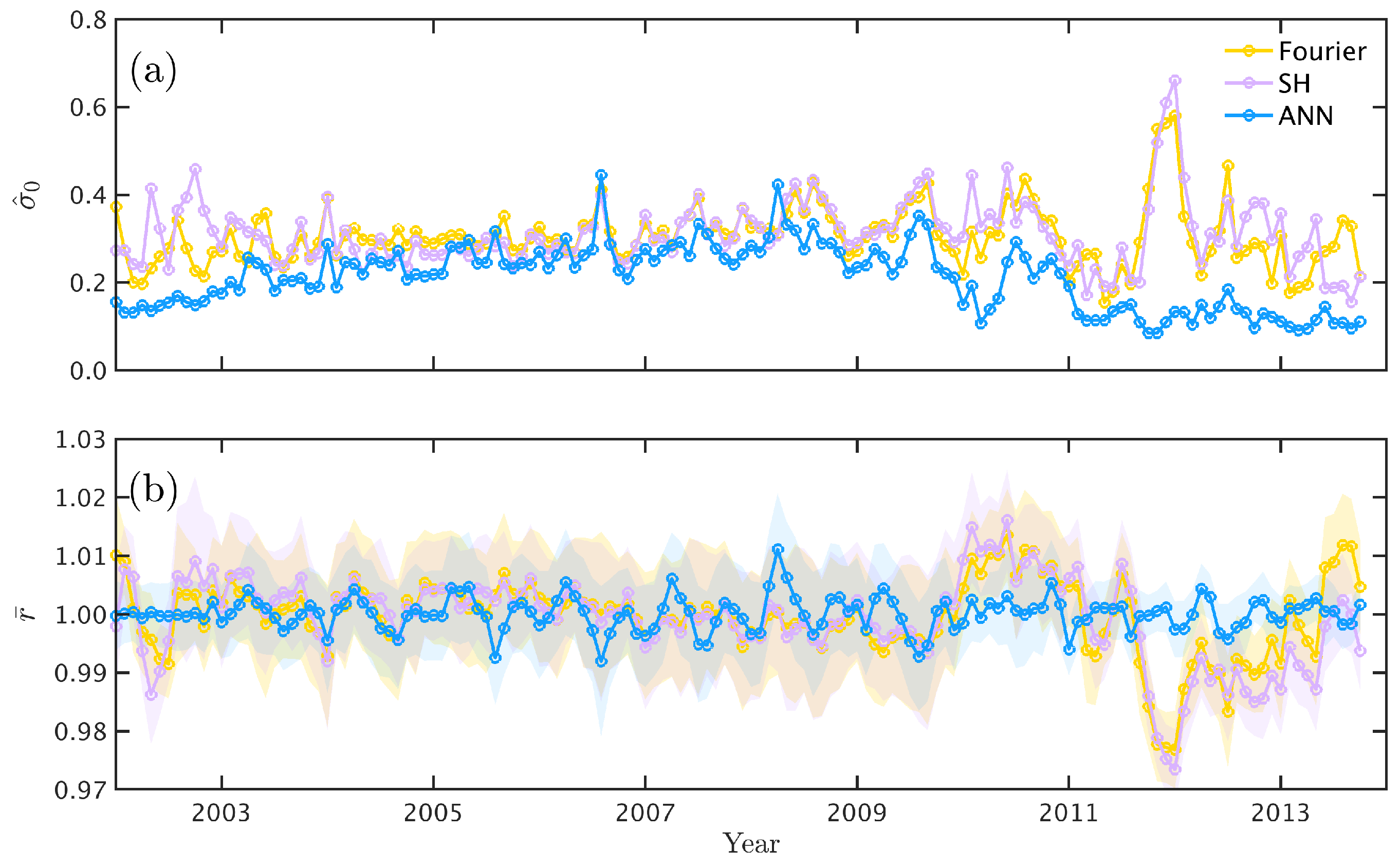
Figure 7 shows comparisons of the Fourier-3 (GSM-LT), SH-1 (QD-LST), and ANN-3 (QD-LST) models with the reference TMD data sets over 2002–2013. The ANN-based model had the highest precision and lowest bias among the three example empirical models. Since dominant variations in TMD are attributed to solar activity [15,38], the performance of the models showed a strong dependency on the solar activity. In this research, the for all models was larger during low solar activity (around 2007) than during high solar activity. The spikes in at the beginning of 2002 and 2012 were caused by the data gap during these years. Interestingly, the ANN-based model did not appear to be affected by this and still showed good consistency.
5. Conclusions
This study delved into the modelling of thermospheric mass density (TMD) during geomagnetic quiet and weakly disturbed time, employing accelerometer-derived TMD observations from four Low Earth Orbit (LEO) satellites: GRACE (∼500 km), CHAMP (∼400 km), and GOCE (∼250 km), spanning the years 2002 to 2013. Various temporal and coordinate representations were scrutinised within the context of empirical TMD models. Furthermore, we explored three modelling methods, namely Fourier analysis, spherical harmonics (SH) analysis, and ANN techniques, to assess their suitability for global TMD modelling. A comprehensive evaluation and validation of these models was conducted to ascertain the optimal method for TMD modelling. The result showed the superiority of the Geocentric Solar Magnetic (GSM) coordinate system in the empirical TMD models. Both Fourier- and SH-based models exhibited limitations in approximating the vertical gradient of TMD. In contrast, the ANN-based model demonstrated a capacity to capture vertical TMD variability without exhibiting sensitivity to the input parameters of time and coordinates.
A significant challenge in TMD modelling lies in accurately approximating the vertical TMD gradient. Two potential solutions emerge: altitude-dependent modelling, which entails constructing multiple models at distinct reference heights, and ANN modelling. The results of this research indicate that the ANN-based models outperformed the Fourier- and SH-based models on three fronts: (1) the ANN-based models adeptly captured vertical TMD variability without necessitating explicit altitude dependency; (2) a sufficiently complex ANN structure, marked by an adequate number of hidden layers and neurons, proved insensitive to variations in time and coordinate frames; (3) the ANN-based models attained higher accuracy when compared to the other two model types.
Furthermore, given that TMD measurements from LEO satellites are obtainable solely along their trajectories, certain spatial features of TMD, such as equatorial mass anomalies (EMAs), are challenging to capture using satellite drag-derived TMD exclusively. In future research, the pursuit of improved metrics may be necessary to address the limitations of existing TMD modelling techniques, particularly when dealing with LEO-satellite-derived measurements.
Author Contributions
Methodology, C.H., A.H. and W.L.; software, C.H., A.H. and W.L.; investigation, C.H. and H.C.; resources, C.H., A.H. and Z.X.; writing, C.H. and Z.X.; funding acquisition, C.H. and D.Z. All authors have read and agreed to the published version of the manuscript.
Funding
This research was supported by the National Natural Science Foundation of China (Grant No. 42004025, 42204030, and 42204037); the Scientific Research Fund of Hunan Provincial Education Department (Grant No. 22C0247); and the 2022 Guangxi University Young and Middle-aged Teachers Research Basic Ability Improvement Project (Grant No. 2022KY0826).
Institutional Review Board Statement
Not applicable.
Informed Consent Statement
Not applicable.
Data Availability Statement
The GOCE-derived TMD data set was kindly provided by Doornbos et al. [11] and is available at https://earth.esa.int/web/guest/missions/esa-operational-eo-missions/goce (accessed on 13 August 2019). The GRACE- and CHAMP-derived thermospheric mass density data used in this study are available from http://tinyurl.com/densitysets (accessed on 13 August 2019). The high-resolution (1 min and 5 min) solar wind OMNIweb database is publicly available at https://omniweb.gsfc.nasa.gov/ow_min.html (accessed on 13 August 2019). The geomagnetic indices and can be obtained at http://isgi.unistra.fr (accessed on 13 August 2019).
Acknowledgments
Eelco Doornbos from Delft University of Technology and Piyush Mehta from West Virginia University are thanked for providing the thermospheric neural mass density data of the GOCE, GRACE, and CHAMP satellites. NASA’s Goddard Space Flight Center (GSFC) is thanked for providing the high-resolution (1 min and 5 min) solar wind OMNIweb database. The International Service of Geomagnetic Indices is thanked for providing the geomagnetic indices. Brett Carter and Lucas Holden from RMIT University are thanked for the invaluable suggestions to this paper.
Conflicts of Interest
The authors declare no conflicts of interest.
Abbreviations
The following abbreviations are used in this manuscript:
| LEO | Low Earth Orbit |
| TMD | Thermospheric mass density |
| SH | Spherical harmonics |
| ANN | Artificial neural network |
Appendix A. The Terms f in the Fourier Model
The terms in Equation (2) representing the vertical, solar activity, geomagnetic, latitudinal, longitudinal, intra-diurnal, and intra-annual variations in TMD are given by
where and are the solar and geomagnetic indices; and are the geographic, solar, or geomagnetic latitudes and longitudes [9], respectively, which are termed as ‘general’ latitudes and longitudes hereafter; h is the altitude; and is the TMD at the reference altitude of . is the hour of the day, and is the day of the year, which can be measured by UT, LT, LST, or MLT. The , , and used by Xiong et al. [14] were the geographic coordinates and MLT, respectively.
Appendix B. The Function G in SH-Based Model
In Equations (4) and (5), the function of is given by
where
and is the non-normalised Legendre polynomials as used in NRLMSISE-00. and are the general latitudes and longitudes, respectively. The terms related to the geomagnetic effect were estimated in the modelling of this study, but the developed models were evaluated at for consistency. See Yamazaki et al. [15] for more explanation. Similar to the Fourier-based model, the model coefficients in Equation (A8) were estimated using a separate Levenberg–Marquardt algorithm, which was also originally used in the development of NRLMSISE-00 [34].
References
- Doornbos, E. Thermospheric Density and Wind Determination from Satellite Dynamics; Springer: Berlin/Heidelberg, Germany, 2012. [Google Scholar] [CrossRef]
- Ruan, H.; Lei, J.; Dou, X.; Liu, S.; Aa, E. An exospheric temperature model based On CHAMP observations and TIEGCM simulations. Space Weather 2018, 16, 147–156. [Google Scholar] [CrossRef]
- Richmond, A.D.; Ridley, E.C.; Roble, R.G. A thermosphere/ionosphere general circulation model with coupled electrodynamics. Geophys. Res. Lett. 1992, 19, 601–604. [Google Scholar] [CrossRef]
- Foster, B. TIEGCM Documentation, Release 2.0; Report; National Center for Atmospheric Research/High Altitude: Boulder, CO, USA, 2016. [Google Scholar]
- Bruinsma, S.; Arnold, D.; Jaggi, A.; Sanchez-Ortiz, N. Semi-empirical thermosphere model evaluation at low altitude with GOCE densities. J. Space Weather. Space Clim. 2017, 7, A4. [Google Scholar] [CrossRef]
- Bowman, B.R.; Tobiska, W.K.; Marcos, F.A.; Huang, C.Y.; Lin, C.S.; Burke, W.J. A new empirical thermospheric density model JB2008 using new solar and geomagnetic indices. In Proceedings of the AIAA/AAS Astrodynamics Specialist Conference and Exhibit, Honolulu, HI, USA, 18–21 August 2008; p. 6438. [Google Scholar] [CrossRef]
- Qian, L.; Solomon, S.C. Thermospheric Density: An Overview of Temporal and Spatial Variations. Space Sci. Rev. 2012, 168, 147–173. [Google Scholar] [CrossRef]
- Emmert, J.T. Thermospheric mass density: A review. Adv. Space Res. 2015, 56, 773–824. [Google Scholar] [CrossRef]
- He, C.; Yang, Y.; Carter, B.; Kerr, E.; Wu, S.; Deleflie, F.; Cai, H.; Zhang, K.; Sagnières, L.; Norman, R. Review and comparison of empirical thermospheric mass density models. Prog. Aerosp. Sci. 2018, 103, 31–51. [Google Scholar] [CrossRef]
- Sutton, E.K. Effects of Solar Disturbances on the Thermosphere Densities and Winds from CHAMP and GRACE Satellite Accelerometer Data. Ph.D. Thesis, Department of Aerospace Engineering Sciences, University of Colorado at Boulder, Boulder, CO, USA, 2008. [Google Scholar]
- Doornbos, E.; Van Den IJssel, J.; Luhr, H.; Forster, M.; Koppenwallner, G. Neutral Density and Crosswind Determination from Arbitrarily Oriented Multiaxis Accelerometers on Satellites. J. Spacecr. Rocket. 2010, 47, 580–589. [Google Scholar] [CrossRef]
- Mehta, P.M.; Walker, A.C.; Sutton, E.K.; Godinez, H.C. New density estimates derived using accelerometers on board the CHAMP and GRACE satellites. Space Weather 2017, 15, 558–576. [Google Scholar] [CrossRef]
- Liu, H.; Hirano, T.; Watanabe, S. Empirical model of the thermospheric mass density based on CHAMP satellite observations. J. Geophys. Res. Space Phys. 2013, 118, 843–848. [Google Scholar] [CrossRef]
- Xiong, C.; Lühr, H.; Schmidt, M.; Bloßfeld, M.; Rudenko, S. An empirical model of the thermospheric mass density derived from CHAMP satellite. Ann. Geophys. 2018, 36, 1141–1152. [Google Scholar] [CrossRef]
- Yamazaki, Y.; Kosch, M.J.; Sutton, E.K. A model of high-latitude thermospheric density. J. Geophys. Res. Space Phys. 2015, 120, 7903–7917. [Google Scholar] [CrossRef]
- Calabia, A.; Jin, S.G. New modes and mechanisms of thermospheric mass density variations from GRACE accelerometers. J. Geophys. Res. Space Phys. 2016, 121, 11191–11211. [Google Scholar] [CrossRef]
- Perez, D.; Wohlberg, B.; Lovell, T.A.; Shoemaker, M.; Bevilacqua, R. Orbit-centered atmospheric density prediction using artificial neural networks. Acta Astronaut. 2014, 98, 9–23. [Google Scholar] [CrossRef]
- Chen, H.; Liu, H.; Hanada, T. Storm-time atmospheric density modeling using neural networks and its application in orbit propagation. Adv. Space Res. 2014, 53, 558–567. [Google Scholar] [CrossRef]
- Pardini, C.; Moe, K.; Anselmo, L. Thermospheric density model biases at the 23rd sunspot maximum. Planet. Space Sci. 2012, 67, 130–146. [Google Scholar] [CrossRef]
- Laundal, K.M.; Gjerloev, J. What is the appropriate coordinate system for magnetometer data when analyzing ionospheric currents? J. Geophys. Res. Space Phys. 2014, 119, 8637–8647. [Google Scholar] [CrossRef]
- Lei, J.; Matsuo, T.; Dou, X.; Sutton, E.; Luan, X. Annual and semiannual variations of thermospheric density: EOF analysis of CHAMP and GRACE data. J. Geophys. Res. Space Phys. 2012, 117, A01310. [Google Scholar] [CrossRef]
- Weimer, D.R.; Sutton, E.K.; Mlynczak, M.G.; Hunt, L.A. Intercalibration of neutral density measurements for mapping the thermosphere. J. Geophys. Res. Space Phys. 2016, 121, 5975–5990. [Google Scholar] [CrossRef]
- Bruinsma, S.; Forbes, J.M.; Nerem, R.S.; Zhang, X. Thermosphere density response to the 20–21 November 2003 solar and geomagnetic storm from CHAMP and GRACE accelerometer data. J. Geophys. Res. 2006, 111, A06303. [Google Scholar] [CrossRef]
- Xu, J.Y.; Wang, W.B.; Gao, H. The longitudinal variation of the daily mean thermospheric mass density. J. Geophys. Res. Space Phys. 2013, 118, 515–523. [Google Scholar] [CrossRef]
- Leonard, J.M.; Forbes, J.M.; Born, G.H. Impact of tidal density variability on orbital and reentry predictions. Space Weather 2012, 10, S12003. [Google Scholar] [CrossRef]
- Shi, C.; Li, W.W.; Li, M.; Zhao, Q.L.; Sang, J.Z. Calibrating the scale of the NRLMSISE00 model during solar maximum using the two line elements dataset. Adv. Space Res. 2015, 56, 1–9. [Google Scholar] [CrossRef]
- Doornbos, E.; Klinkrad, H.; Visser, P. Use of two-line element data for thermosphere neutral density model calibration. Adv. Space Res. 2008, 41, 1115–1122. [Google Scholar] [CrossRef]
- Laundal, K.M.; Richmond, A.D. Magnetic Coordinate Systems. Space Sci. Rev. 2017, 206, 27–59. [Google Scholar] [CrossRef]
- He, C. Precise Thermospheric Mass Density Modelling for Orbit Prediction of Low Earth Orbiters. Ph.D. Thesis, RMIT University, Melbourne, Australia, 2019. [Google Scholar]
- Marquardt, D.W. An algorithm for least-squares estimation of nonlinear parameters. J. Soc. Ind. Appl. Math. 1963, 11, 431–441. [Google Scholar] [CrossRef]
- Drob, D.P.; Emmert, J.T.; Crowley, G.; Picone, J.M.; Shepherd, G.G.; Skinner, W.; Hays, P.; Niciejewski, R.J.; Larsen, M.; She, C.Y.; et al. An empirical model of the Earth’s horizontal wind fields: HWM07. J. Geophys. Res. Space Phys. 2008, 113, A12304. [Google Scholar] [CrossRef]
- Drob, D.P.; Emmert, J.T.; Meriwether, J.W.; Makela, J.J.; Doornbos, E.; Conde, M.; Hernandez, G.; Noto, J.; Zawdie, K.A.; McDonald, S.E.; et al. An update to the Horizontal Wind Model (HWM): The quiet time thermosphere. Earth Space Sci. 2015, 2, 301–319. [Google Scholar] [CrossRef]
- He, C.; Wu, S.; Wang, X.; Hu, A.; Wang, Q.; Zhang, K. A new voxel-based model for the determination of atmospheric weighted mean temperature in GPS atmospheric sounding. Atmos. Meas. Tech. 2017, 10, 2045–2060. [Google Scholar] [CrossRef]
- Picone, J.M.; Hedin, A.E.; Drob, D.P.; Aikin, A.C. NRLMSISE-00 empirical model of the atmosphere: Statistical comparisons and scientific issues. J. Geophys. Res. Space Phys. 2002, 107, 1468. [Google Scholar] [CrossRef]
- Chen, J.; Li, W.; Li, S.; Chen, H.; Zhao, X.; Peng, J.; Chen, Y.; Deng, H. Two-Stage Solar Flare Forecasting Based on Convolutional Neural Networks. Space: Sci. Technol. 2022, 2022, 9761567. [Google Scholar] [CrossRef]
- Li, W.; Liu, L.; Chen, Y.; Xiao, Z.; Le, H.; Zhang, R. Improving the Extraction Ability of Thermospheric Mass Density Variations From Observational Data by Deep Learning. Space Weather 2023, 21, e2022SW003376. [Google Scholar] [CrossRef]
- Li, W.; Zhao, D.; He, C.; Shen, Y.; Hu, A.; Zhang, K. Application of a Multi-Layer Artificial Neural Network in a 3-D Global Electron Density Model Using the Long-Term Observations of COSMIC, Fengyun-3C, and Digisonde. Space Weather 2021, 19, e2020SW002605. [Google Scholar] [CrossRef]
- Emmert, J.T.; Picone, J.M. Climatology of globally averaged thermospheric mass density. J. Geophys. Res. Space Phys. 2010, 115, A09326. [Google Scholar] [CrossRef]
Figure 1.
Model-to-observation ratio of TMD during geomagnetic quiet and weakly disturbed time from 2002 to 2013. The reference model used here was NRLMSISE-00. See Section 2.1 for more details on the data selection. The GOCE TMD data were provided by Doornbos [1], and the other data were provided by Mehta et al. [12]. The legend is shared among all the panels.
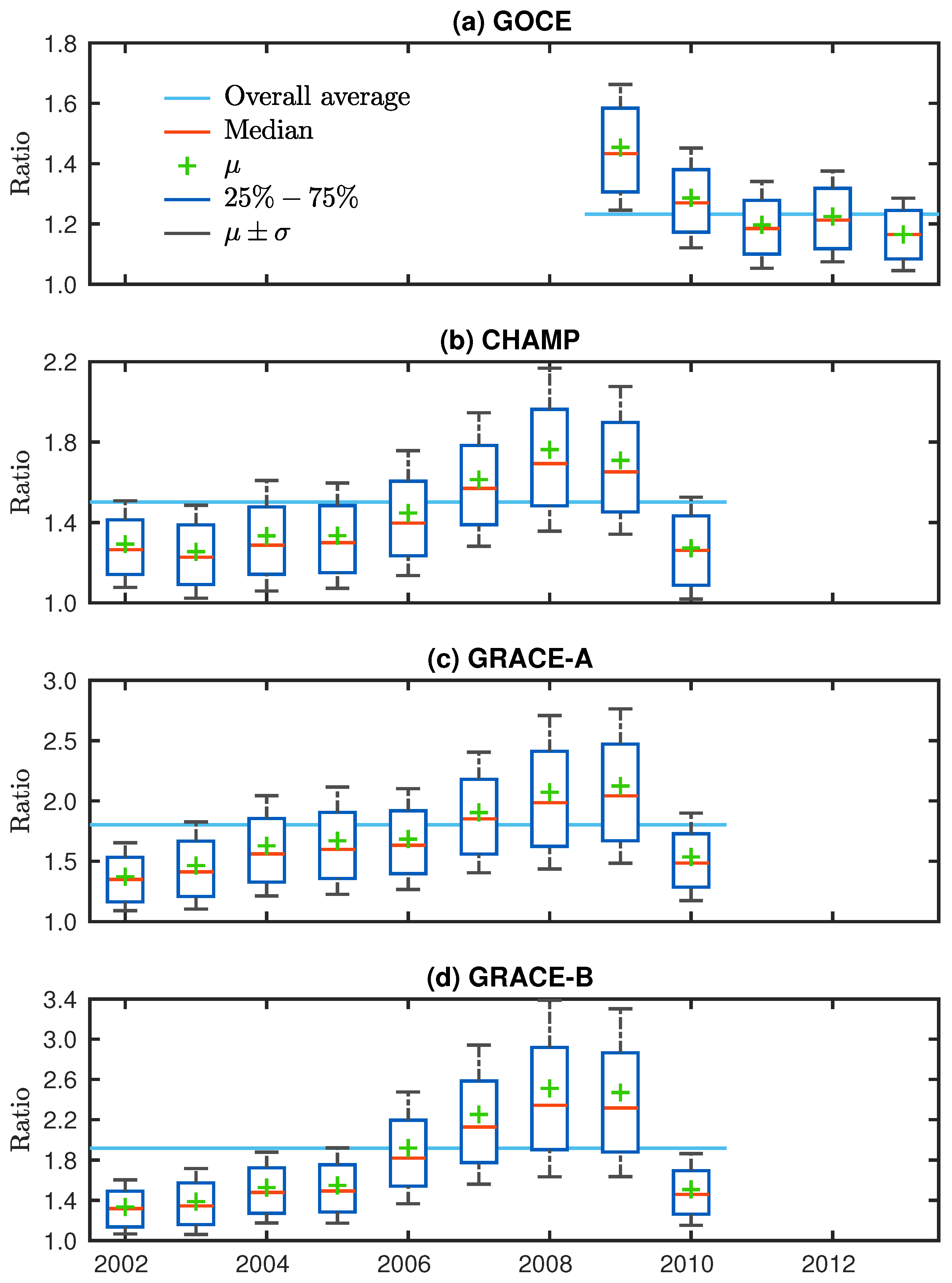
Figure 2.
Pearson correlation coefficients between accelerometer-derived TMD and solar indices of (a) daily average and (b) last 81–day average during quiet and weakly disturbed time. Solar indices considered include the sunspot number, , Lyman–α, Mg II, , and . Scaled TMD data sets from GRACE-A/B, CHAMP, and GOCE were daily averaged and normalised to the altitude of km using NRLMSISE-00. The curve of Mg II is completely overlapped by that of due to their linearity. The legend is shared between the top and bottom panels.
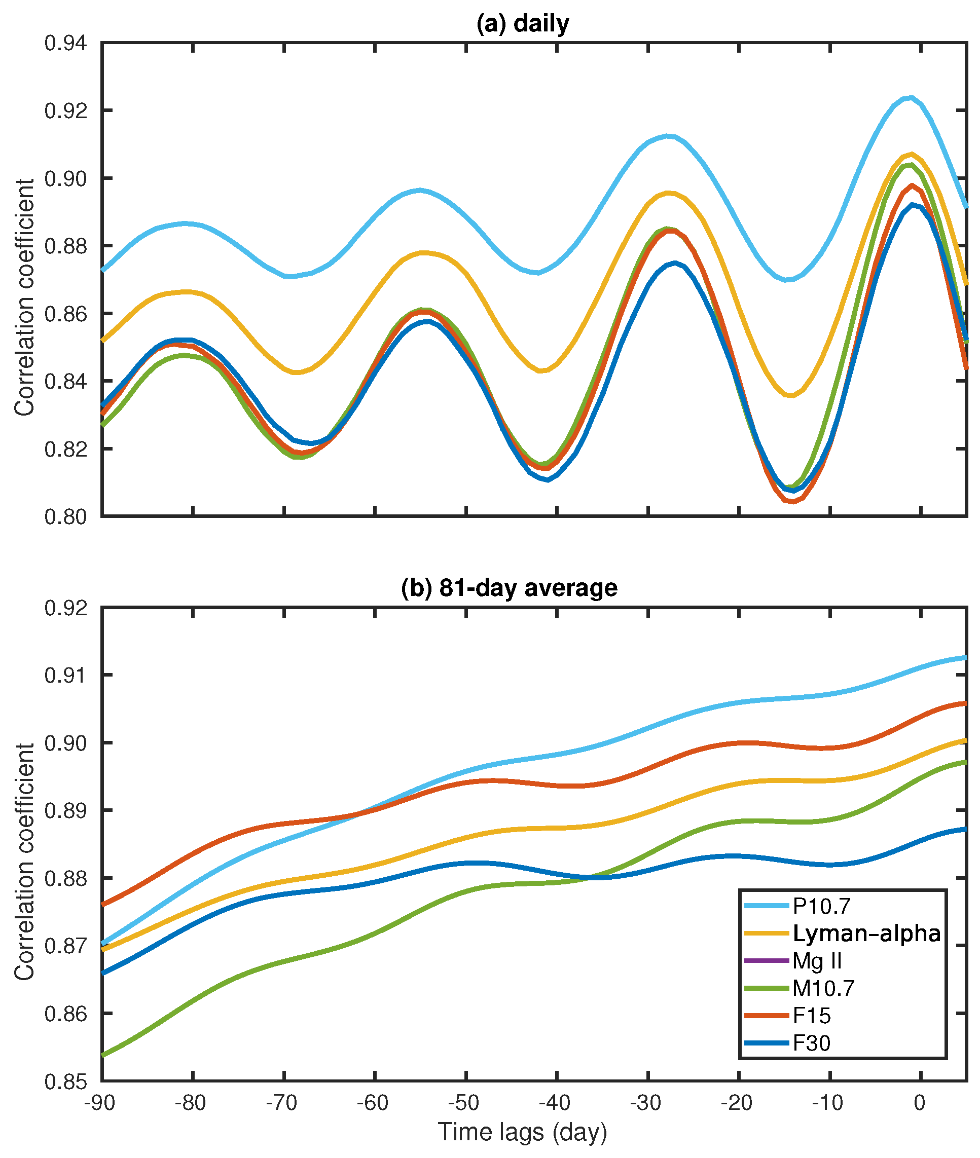
Figure 3.
Pearson correlation coefficients between accelerometer–derived TMD and geomagnetic and solar wind indices of (a) daily average and (b) last 81–day average during quiet and weakly disturbed time. Considered geomagnetic indices include ; ; ; ; ; ; ; IMF (inter–planetary magnetic field) components; and solar wind plasma parameters (flow pressure, temperature, speed, and proton density). Note that the index was provided by NASA OMNI2. The legend is shared between the top and bottom panels.
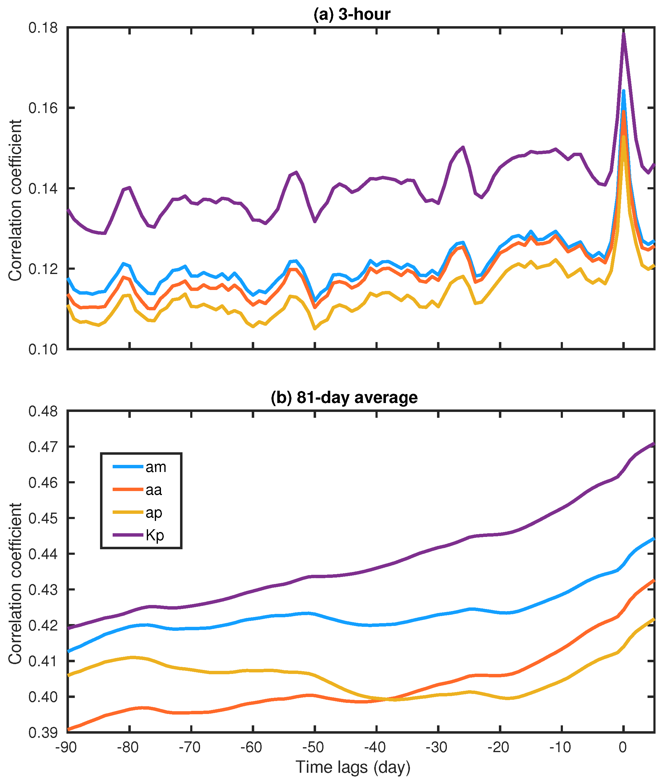
Figure 4.
Comparisons of the Fourier (GSM-LT) model between the observed and predicted TMD in the unit of for (a) GRACE-A, (b) GRACE-B, (c) CHAMP, and (d) GOCE. The red lines depict the linear regression result. The colour bar shows the year of the TMD data.
Figure 4.
Comparisons of the Fourier (GSM-LT) model between the observed and predicted TMD in the unit of for (a) GRACE-A, (b) GRACE-B, (c) CHAMP, and (d) GOCE. The red lines depict the linear regression result. The colour bar shows the year of the TMD data.
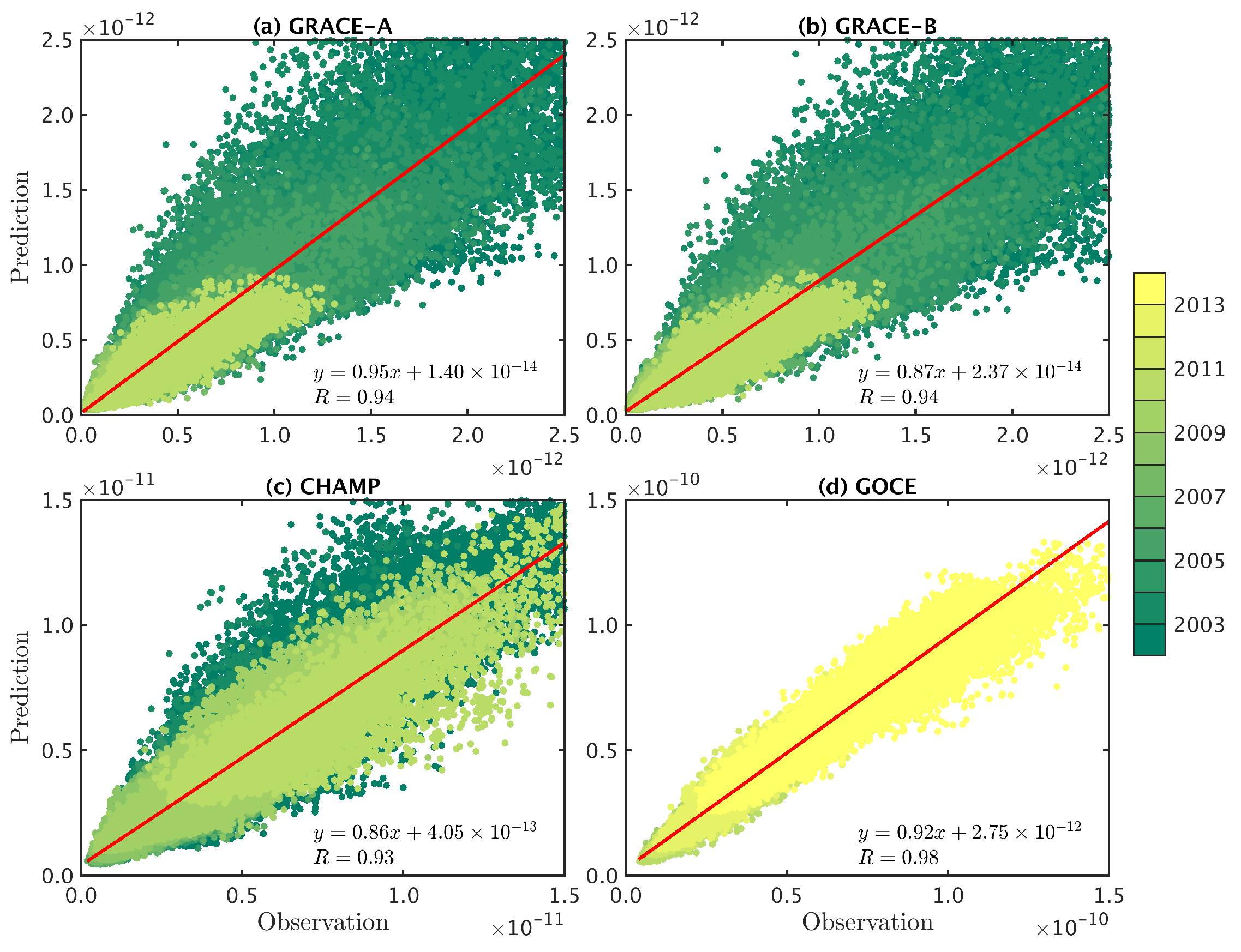
Figure 5.
Distribution of residuals (left) and the quantile–quantile plot (right) for the ANN-1 model from GRACE-A/B, CHAMP, and GOCE. The number of neurons in the single hidden layer was 100. The TMD error is in the unit of .
Figure 5.
Distribution of residuals (left) and the quantile–quantile plot (right) for the ANN-1 model from GRACE-A/B, CHAMP, and GOCE. The number of neurons in the single hidden layer was 100. The TMD error is in the unit of .
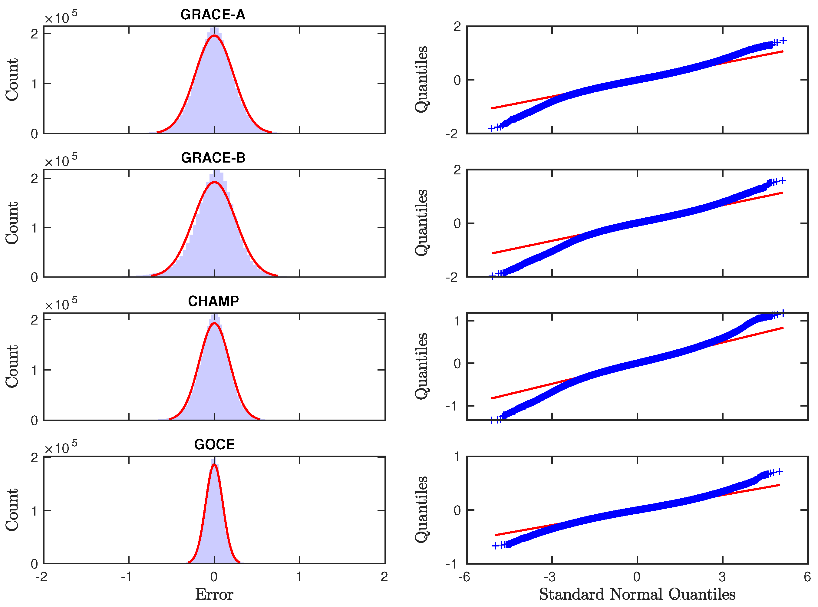
Figure 6.
The QD latitude versus LST distribution of TMD predicted by ANN-based model at km around March equinox during solar maximum (left column, ) and solar minimum (right column, ). The panels (a,b) were predicted by ANN-1(50); (c,d) by ANN-2(20); and (e,f) by ANN-3(20-20-10). The digits in the parenthesis represent the number of neurons in the hidden layer(s). The colour bars indicate the TMD in the unit of 10−11 kg m−3.
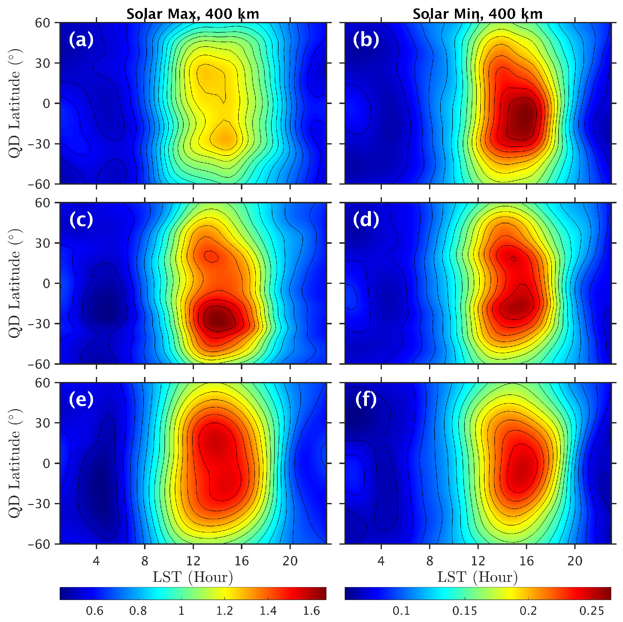
Figure 7.
Comparisons of (a) the a posteriori STD and (b) TMD ratio among the Fourier-4 (GSM-LT, in yellow); SH-1 (QD-LST, in purple); and ANN-3 (QD-LST, in blue) models. Reference TMD was inferred from GRACE-A/B, CHAMP, and GOCE. The shaded area in the bottom panel indicates the one-STD range. The legend is shared between the two panels.

Table 1.
Details of the Fourier-, SH-, and ANN-based models. ANN-1 and ANN-2 are single-hidden-layer ANN models, and ANN-3 has three hidden layers. The number of neurons in the hidden layer(s) is given in the fifth column.
Table 1.
Details of the Fourier-, SH-, and ANN-based models. ANN-1 and ANN-2 are single-hidden-layer ANN models, and ANN-3 has three hidden layers. The number of neurons in the hidden layer(s) is given in the fifth column.
| Model | Inputs | No. Inputs | No. Coefficients | No. Neurons |
|---|---|---|---|---|
| Fourier | , , h, , , , | 7 | 170 | |
| SH-1 | , , h, , , , | 7 | 102 | |
| SH-2 | , , h, , , , | 7 | 300 | |
| ANN-1 | ,, h, , , , , , , , | 11 | 66 | 5 |
| 131 | 10 | |||
| 261 | 20 | |||
| 651 | 50 | |||
| 1301 | 100 | |||
| ANN-2 | , , h, , (), , (), , (), , () | 33 | 176 | 5 |
| 351 | 10 | |||
| 701 | 20 | |||
| 1751 | 50 | |||
| 3501 | 100 | |||
| ANN-3 | , , h, , , , , , , , | 11 | 291 | 10-10-5 |
| 506 | 15-15-5 | |||
| 591 | 15-15-10 | |||
| 881 | 20-20-10 | |||
| 991 | 20-20-15 |
Table 2.
The a posteriori STD of unit weight ( of the Fourier model for the four satellites in the unit of . The model was built at five reference heights of 250, 300, 400, 500, and km. For simplicity, only the results of five coordinate and time frames are presented.
Table 2.
The a posteriori STD of unit weight ( of the Fourier model for the four satellites in the unit of . The model was built at five reference heights of 250, 300, 400, 500, and km. For simplicity, only the results of five coordinate and time frames are presented.
| Coordinate–Time | GRACE-A | GRACE-B | CHAMP | GOCE | Overall |
|---|---|---|---|---|---|
| GEO-LST | 0.3338 | 0.3712 | 0.2890 | 0.1354 | 0.3099 |
| GEO-MLT | 0.3410 | 0.3765 | 0.2842 | 0.1465 | 0.3133 |
| GSM-LT | 0.3030 | 0.3390 | 0.2353 | 0.1140 | 0.2742 |
| GSM-LST | 0.3011 | 0.3353 | 0.2260 | 0.1193 | 0.2704 |
| QD-LST | 0.3331 | 0.3705 | 0.2891 | 0.1363 | 0.3095 |
Table 3.
The a posteriori STD of unit weight (, unit: ) of the SH-1 model. Values in bold show the best fitting result. MLT for GEO, GSM, SM, and DIP frames was derived from the QD longitude.
Table 3.
The a posteriori STD of unit weight (, unit: ) of the SH-1 model. Values in bold show the best fitting result. MLT for GEO, GSM, SM, and DIP frames was derived from the QD longitude.
| Coordinates | Time | ||
|---|---|---|---|
| LT | LST | MLT | |
| GEO | 0.3147 | 0.3146 | 0.3173 |
| GSM | 0.3102 | 0.3103 | 0.3110 |
| SM | 0.3185 | 0.3184 | 0.3173 |
| DIP | 0.3242 | 0.3241 | 0.3274 |
| CD | 0.3162 | 0.3162 | 0.3162 |
| ED | 0.3169 | 0.3168 | 0.3165 |
| QD | 0.3174 | 0.3173 | 0.3165 |
| MA | 0.3174 | 0.3173 | 0.3165 |
Table 4.
The a posteriori STD of unit weight (, unit: ) of the SH-2 model. The model was built at five reference heights of 200, 300, and km.
Table 4.
The a posteriori STD of unit weight (, unit: ) of the SH-2 model. The model was built at five reference heights of 200, 300, and km.
| Coordinate–Time | GRACE-A | GRACE-B | CHAMP | GOCE | Overall |
|---|---|---|---|---|---|
| GEO-LT | 0.2716 | 0.3085 | 0.2261 | 0.1592 | 0.2557 |
| GEO-LST | 0.2711 | 0.3079 | 0.2248 | 0.1630 | 0.2554 |
| GEO-MLT | 0.2745 | 0.3114 | 0.2264 | 0.1639 | 0.2580 |
| GSM-LT | 0.2677 | 0.3032 | 0.2211 | 0.1580 | 0.2514 |
| GSM-LST | 0.2678 | 0.3033 | 0.2211 | 0.1583 | 0.2515 |
| QD-LST | 0.2762 | 0.3130 | 0.2287 | 0.1614 | 0.2594 |
Table 5.
The a posteriori STD of unit weight (, unit: ); mean TMD ratio (); and Pearson correlation coefficient (R) of ANN-1 model.
Table 5.
The a posteriori STD of unit weight (, unit: ); mean TMD ratio (); and Pearson correlation coefficient (R) of ANN-1 model.
| Coordinate–Time | Neurons in Hidden Layer | R | ||
|---|---|---|---|---|
| GEO-LST | 5 | 0.2718 | 1.0392 | 0.9881 |
| 10 | 0.2419 | 1.0307 | 0.9882 | |
| 20 | 0.2255 | 1.0267 | 0.9927 | |
| 50 | 0.2085 | 1.0226 | 0.9948 | |
| 100 | 0.2019 | 1.0211 | 0.9954 | |
| GSM-LT | 5 | 0.2501 | 1.0332 | 0.9922 |
| 10 | 0.2442 | 1.0315 | 0.9878 | |
| 20 | 0.2234 | 1.0283 | 0.9943 | |
| 50 | 0.2117 | 1.0233 | 0.9949 | |
| 100 | 0.2053 | 1.0218 | 0.9952 | |
| QD-LST | 5 | 0.2656 | 1.0374 | 0.9882 |
| 10 | 0.2393 | 1.0302 | 0.9902 | |
| 20 | 0.2252 | 1.0264 | 0.9936 | |
| 50 | 0.2111 | 1.0256 | 0.9946 | |
| 100 | 0.2028 | 1.0226 | 0.9952 |
Table 6.
The a posteriori STD of unit weight (, unit: ); mean TMD ratio (); and Pearson correlation coefficient (R) of ANN-2 model.
Table 6.
The a posteriori STD of unit weight (, unit: ); mean TMD ratio (); and Pearson correlation coefficient (R) of ANN-2 model.
| Coordinate–Time | Neurons in Hidden Layers | R | ||
|---|---|---|---|---|
| GEO-LST | 5 | 0.2426 | 1.0309 | 0.9918 |
| 10 | 0.2202 | 1.0251 | 0.9931 | |
| 20 | 0.2117 | 1.0229 | 0.9948 | |
| 50 | 0.2027 | 1.0213 | 0.9952 | |
| 100 | 0.1920 | 1.0199 | 0.9955 | |
| GSM-LT | 5 | 0.2391 | 1.0302 | 0.9906 |
| 10 | 0.2216 | 1.0259 | 0.9931 | |
| 20 | 0.2125 | 1.0234 | 0.9946 | |
| 50 | 0.2013 | 1.0208 | 0.9951 | |
| 100 | 0.1904 | 1.0189 | 0.9950 | |
| QD-LST | 5 | 0.2447 | 1.0316 | 0.9911 |
| 10 | 0.2392 | 1.0307 | 0.9898 | |
| 20 | 0.2143 | 1.0241 | 0.9948 | |
| 50 | 0.2006 | 1.0207 | 0.9951 | |
| 100 | 0.1959 | 1.0199 | 0.9950 |
Table 7.
The a posteriori STD of unit weight (, unit: ); mean TMD ratio (); and Pearson correlation coefficient (R) of ANN-3 model.
Table 7.
The a posteriori STD of unit weight (, unit: ); mean TMD ratio (); and Pearson correlation coefficient (R) of ANN-3 model.
| Coordinate–Time | Neurons in Hidden Layers | R | ||
|---|---|---|---|---|
| GEO-LST | 10-10-5 | 0.2159 | 1.0242 | 0.9949 |
| 15-15-5 | 0.2077 | 1.0224 | 0.9951 | |
| 15-15-10 | 0.2047 | 1.0218 | 0.9953 | |
| 20-20-10 | 0.2032 | 1.0217 | 0.9956 | |
| 20-20-15 | 0.2032 | 1.0208 | 0.9954 | |
| GEO-MLT | 10-10-5 | 0.2216 | 1.0255 | 0.9950 |
| 15-15-5 | 0.2114 | 1.0238 | 0.9953 | |
| 15-15-10 | 0.2106 | 1.0230 | 0.9953 | |
| 20-20-10 | 0.2049 | 1.0239 | 0.9955 | |
| 20-20-15 | 0.2032 | 1.0212 | 0.9957 | |
| GSM-LST | 10-10-5 | 0.2199 | 1.0253 | 0.9942 |
| 15-15-5 | 0.2100 | 1.0229 | 0.9952 | |
| 15-15-10 | 0.2087 | 1.0227 | 0.9951 | |
| 20-20-10 | 0.2038 | 1.0216 | 0.9953 | |
| 20-20-15 | 0.2032 | 1.0202 | 0.9954 | |
| QD-LST | 10-10-5 | 0.2166 | 1.0235 | 0.9943 |
| 15-15-5 | 0.2084 | 1.0221 | 0.9951 | |
| 15-15-10 | 0.2076 | 1.0240 | 0.9952 | |
| 20-20-10 | 0.2041 | 1.0221 | 0.9954 | |
| 20-20-15 | 0.2032 | 1.0219 | 0.9953 |
Disclaimer/Publisher’s Note: The statements, opinions and data contained in all publications are solely those of the individual author(s) and contributor(s) and not of MDPI and/or the editor(s). MDPI and/or the editor(s) disclaim responsibility for any injury to people or property resulting from any ideas, methods, instructions or products referred to in the content. |
© 2024 by the authors. Licensee MDPI, Basel, Switzerland. This article is an open access article distributed under the terms and conditions of the Creative Commons Attribution (CC BY) license (https://creativecommons.org/licenses/by/4.0/).
Share and Cite
MDPI and ACS Style
He, C.; Li, W.; Hu, A.; Zheng, D.; Cai, H.; Xiong, Z. Thermospheric Mass Density Modelling during Geomagnetic Quiet and Weakly Disturbed Time. Atmosphere 2024, 15, 72. https://doi.org/10.3390/atmos15010072
AMA Style
He C, Li W, Hu A, Zheng D, Cai H, Xiong Z. Thermospheric Mass Density Modelling during Geomagnetic Quiet and Weakly Disturbed Time. Atmosphere. 2024; 15(1):72. https://doi.org/10.3390/atmos15010072
Chicago/Turabian StyleHe, Changyong, Wang Li, Andong Hu, Dunyong Zheng, Han Cai, and Zhaohui Xiong. 2024. "Thermospheric Mass Density Modelling during Geomagnetic Quiet and Weakly Disturbed Time" Atmosphere 15, no. 1: 72. https://doi.org/10.3390/atmos15010072
Note that from the first issue of 2016, this journal uses article numbers instead of page numbers. See further details here.