
ECMWF Lightning Forecast in Mainland Portugal during Four Fire Seasons
by
 , ,
, ,
Cátia Campos
1,*,
Flavio T. Couto
1,2,
Filippe L. M. Santos
1,
João Rio
3,
Teresa Ferreira
3 and
Rui Salgado
1,2 1
Earth Remote Sensing Laboratory (EaRS Lab), Institute of Earth Sciences—ICT, Instituto de Investigação e Formação Avançada—IIFA, University of Évora, Rua Romão Ramalho 59, 7000-671 Évora, Portugal
2
Department of Physics, School of Science and Technology, University of Évora, Rua Romão Ramalho 59, 7000-671 Évora, Portugal
3
Portuguese Institute for Sea and Atmosphere, I.P., Rua C do Aeroporto, 1749-077 Lisbon, Portugal
*
Author to whom correspondence should be addressed.
Atmosphere 2024, 15(2), 156; https://doi.org/10.3390/atmos15020156
Submission received: 20 December 2023
/
Revised: 18 January 2024
/
Accepted: 22 January 2024
/
Published: 25 January 2024
(This article belongs to the Section Meteorology)
Abstract
:The study evaluated the ECMWF model ability in forecasting lightning in Portugal during four fire seasons (2019–2022). The evaluation was made based on lightning data from the national lightning detector network, which was aggregated into resolutions of 0.5° and 1° over 3 h periods and analyzed from statistical indices using two contingency tables. The results showed that the model overestimates the lightning occurrence, with a BIAS greater than 1, with a success rate of 57.7% (49%) for a horizontal resolution of 1° (0.5°). The objective analysis was complemented by the spatial lightning distribution analysis, which indicated a time lag between the two data, i.e., the model started predicting lightning before its occurrence and finished the prediction earlier. Furthermore, such analysis revealed the lightning distribution being consistent with some weather patterns. The findings of this study provide insights into the applicability of the ECMWF lightning forecast data in the context of forecasting natural forest fires in Portugal.
1. Introduction
Wildfires result from a combination of several factors, such as weather conditions, climate variability, terrain aspects, as well as the type and amount of vegetation available to burn. Southern European countries such as Portugal, Spain, Greece, and Italy, characterized by having a Mediterranean climate, are among the ones most affected by wildfires in summer, and several studies suggest that climate change may alter wildfire activity behavior in this region (e.g., [1,2]). For instance, January 2022 was the winter month with the highest number of fire outbreaks in Portugal, also indicating possible changes in the fire activity regime [3,4]. Portugal has a long history of forest fires, with the most critical years in terms of total burned area being 2003, 2005, and 2017. In 2017, 11 mega-fires (i.e., forest fires with total burned area above 10,000 hectares [5]) led to over 100 fatalities (e.g., [6,7,8,9,10]). After the year 2017, 2022 was the worst in terms of total burned area, with two fire outbreaks in the regions of Beira and Serra da Estrela [4].
Overall, most of the ignitions in Southern Europe are due to anthropogenic causes [11,12,13], with natural fires, caused by lightning, representing only 5–10% of ignitions in Europe. In Portugal, natural fires are a small ignition percentage compared to other causes [14,15]. While the percentage is about 1.1%, it accounts for 7.5% in the total burned area. For instance, dry thunderstorms in Portugal were responsible for starting 18 wildfires from lightning strikes [15]. More recently, in 2020, the Lousã fire was ignited by lightning from a mesoscale convective system [16].
Ramos et al. [17] analyzed lightning activity over mainland Portugal during the period 2003–2009 and found three main weather patterns: frontal activity, cut-off lows and summer thermal lows. The frontal activity is mostly relevant in the winter season, as storms are formed in the Atlantic Ocean and are advected toward Portuguese territory. In summer, lightning is mostly linked to either cut-offs or daytime convection. The same authors show that summer and autumn are the seasons with more lightning density. Furthermore, the natural ignitions over the Iberia Peninsula normally occur at high elevations (above 1000 m) and under low moisture fuel conditions [18].
The lightning strikes occur in response to a local build-up of an atmospheric electric field. Inside a convective region, the updrafts and downdrafts give rise to the separation of positive and negative electric charges. The electric charges separation happens due to the interaction between hydrometeors with different fall speeds, namely the collision between the graupel or hail particles with ice particles or liquid water droplets. Once a large electric field is produced, a lightning discharge can be triggered [19]. Lightning can also be classified as cloud-to-ground (CG) or intra-cloud (IC). The IC type represents 80% of total discharges, whereas the CG type, even with lower frequency, has more impact on human activity (e.g., natural fires, aviation). Krause et al. [20] studied the impact of climate change on lightning activity in the fire regime and suggested that the CG frequency flash rate should increase by 21% at the end of century.
Most natural fires occur in the summer season, when a set of factors favor convection and the consequent charges generation from cloud development. In general, the thermodynamic environment of the atmosphere is characterized by hot and dry air at lower levels, followed by a moist layer in the middle troposphere (e.g., [8,9]). As it occurs over a low moist layer, the precipitating systems developed, also known as “dry thunderstorms”, do not have significant precipitation associated [21,22], being a greater fire risk when lightning occurs. On the other hand, large-scale circulation can produce drier and hotter periods, creating favorable conditions to fire activity and acting as an enhancing or suppressing agent (e.g., [9,23]).
In the natural forest fires context, the ability to realistically predict the probability of lightning occurrence can be useful for anticipating these events. Machine learning approaches have been developed in recent years to provide nowcasting of lightning [24,25].
Regarding NWP-based forecasting, there are schemes incorporating cloud-resolving models coupled with electrification models (e.g., MesoNH/CELLS [26,27], WRF/WRF-E [28,29]). For instance, the Meso-NH/CELLS [26,27], successfully represented the lightning strikes occurrence over Pedrógão Grande region in June 2017 [8]. Both models explicitly calculate the atmospheric electric field based on detailed cloud microphysical processes, which makes the computational cost very high. Another approach includes diagnostic schemes that parameterize the number of flashes as function of the hydrometeors distribution and other parameters computed by the cloud-resolving models, as documented in Price and Rind [30], Yair et al. [31], or McCaul et al. [32]. Other schemes use thermodynamic indices, as reported in Bright et al. [33]. Additionally, there are studies employing intermediate levels of complexity, such as Federico et al. [34], who uses the dynamic lightning scheme described in Lynn et al. [35]. This scheme uses the dynamic and microphysics fields from WRF to calculate electrical potential energies for lightning, whose evolution is then the subject of prognostic equations.
Since mid-2018, the European Center for Medium-Range Weather Forecasts (ECMWF) integrated forecast system (IFS) has included a recent parameterization [19] that makes a diagnostic forecast of total lightning density, with lower computational costs. Therefore, the study aims to evaluate the forecast skill of total lightning density from ECMWF in four fire seasons over Portugal.
2. Data and Methods
2.1. Study Area
Portugal (Figure 1) has a Mediterranean climate characterized by a hot and dry summer and a mild and rainy winter months season. Given that wildfires occur mainly in mainland Portugal in summer, this study considers a dataset for June–September, between 2019 and 2022.
2.2. Lightning Data
2.2.1. Lightning Forecast Data
Lightning forecast was provided by ECMWF and has been available since mid-2018. Lopez [19] proposed a parameterization to compute the total lightning density in function of the total amount of convective hydrometeors and some variables diagnosed from the IFS convection scheme. The model takes into account the CAPE (J/kg), the vertical profile of the convective flow of frozen precipitation (Pf; kg/m2s), the specific densities of snow and graupel (kg/kg), the liquid water mixing ratio profile (kg/kg) inside cumuliform clouds, and the convective cloud base height (Zbase, km). The respective graupel and snow densities are diagnosed from the frozen precipitation partition Pf at each vertical model level (see Equations (1) and (2) from Lopez [19]). The current parameterization version does not estimate the intensity or distinguish between IC and CG lightning. The total lightning flash density (flash/km2day) is given by:
where α is a parameter obtained from the calibration based on climatological data, and it is set by Lopez (2016) [19] as 32.40. QR represents the charging rate resulting from the hydrometers collisions [19]. While the ECMWF forecast unit is provided in flash/km2/day, this study considers flashes/100 km2/h to increase forecast interpretation [36].
The forecast data are taken from the 0000 UTC with a maximum range of 24 h, and for June to September, in 2019–2022. The IFS operational version was used with a horizontal resolution of 0.125°. Due to the uncertainty associated with convection, ECMWF recommends using forecasts for extended validation periods, in the order of 6 h (e.g., [37]). Thus, this study considers the total lightning density in the earlier 3 h, that is, the lightning average rate produced in the 3 h prior to the forecast time.
2.2.2. Lightning Observation
The data were provided by the lightning detection network provided by the Instituto Português do Mar e da Atmosfera (I.P., IPMA). The data period is the same as the one from ECMWF, and it is presented in an irregular grid, covering the Portuguese region.
The current lightning detection system in mainland Portugal comprises five VAISALA detectors model LS7002 [38] located in Lisbon, Olhão, Santa Cruz, Castelo Branco, Braga, and Bragança. These detectors operate within a network that includes detectors owned by the Spanish State Meteorological Agency (AEMET), situated near the Portuguese–Spanish border in Santiago, Matacan, Talavera, Jerez, Almagro, and Armilla. The detection and localization principle depends on measuring the frequency of waves emitted by lightning, determining their arrival times at each detector, and applying triangulation to calculate the locations of discharges [39].
The sensor network can detect electrical discharges with a maximum accuracy of 250 m, boasting an efficiency of 95% for CG lightning and 50% for IC lightning [38]. The system provides information on the geographic coordinates of the discharge location, the date and time of occurrence with millisecond resolution, discharge type, polarity, electric current intensity, multiplicity, location calculation method, statistical information (χ2), location error (expressed by parameters of an ellipse), rise time and peak-to-zero time of the waveform, and the number of detectors involved in the location calculation [40]. However, for the purposes of this study, only information about the date and geographic coordinates was considered.
The lightning detection system incorporates a validation algorithm, developed by the VAISALA, which considers several parameters, including location error and its reliability (expressed through the parameter χ2). At IPMA (Lisbon, Portugal) a Total Lightning Processor (TLP) and a Computer Aided Thunderstorm Surveillance (CATS) systems allow real-time collection, archiving, and visualization of lightning detected and located by all the detectors mentioned previously [39].
2.3. Statistical Analysis: Data Processing
Since the goal of this study is to evaluate the lightning forecasts by confronting them with observational data, a quantitative comparison between the ECMWF predictions and IPMA network observations was made. As previously stated, the observed data mesh has an irregular grid, so the first step was to interpolate the observed data on to the forecast grid, which has a spatial resolution of 0.125° and covers mainland Portugal with 25 × 41 grid points (Figure 2). Also, the observation was aggregated for the same periods (3 h) as the ECMWF lightning forecast data. Since the model does not distinguish between IC and CG lightning or estimate their intensities, the observation was reduced to the number of flashes at each grid point: this means that several flashes at the same point can be reduced to just one grid point, as shown in Figure 2.
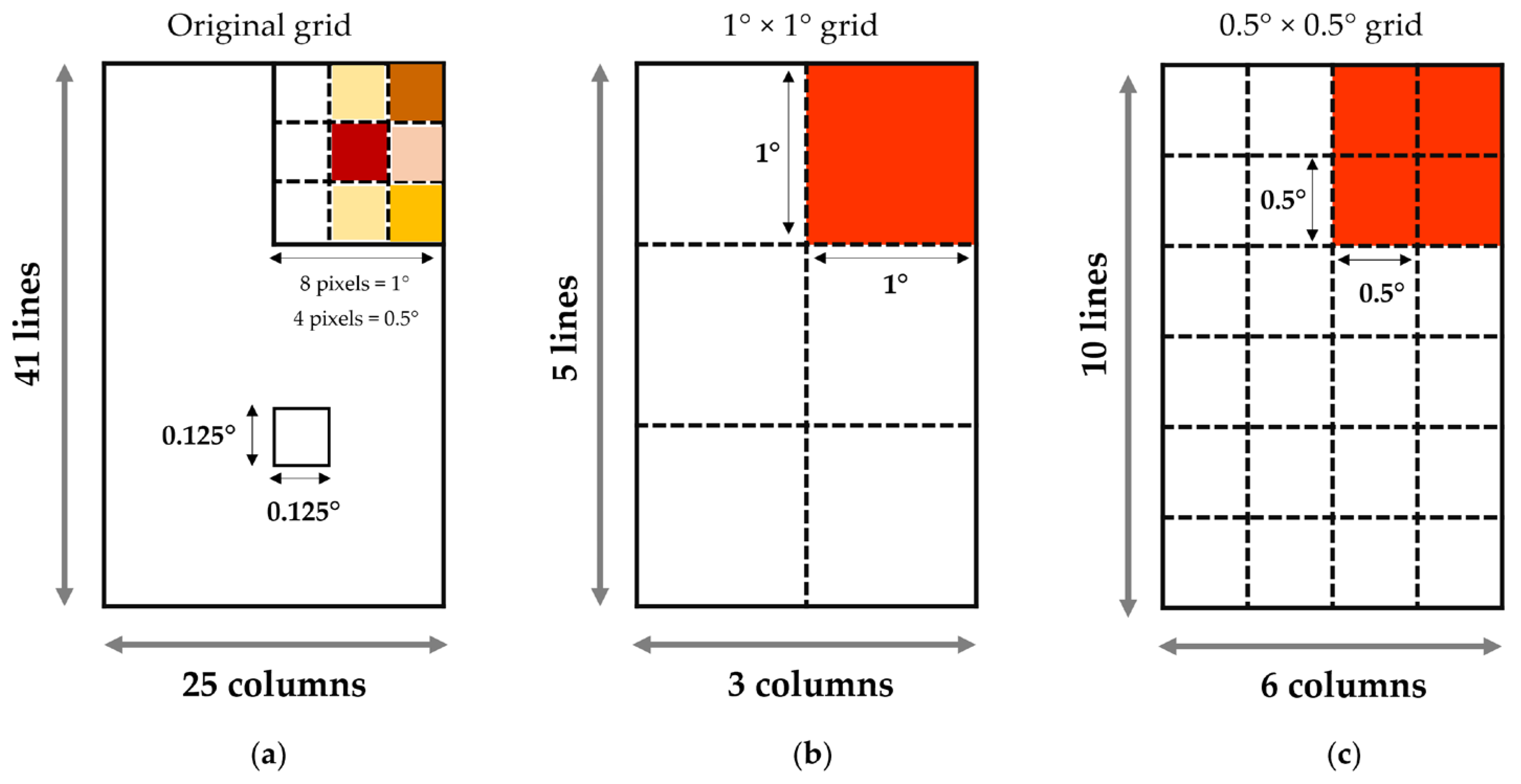
Given the uncertainty associated with the current lightning forecast and the physical difficulty in predicting the flashes trajectory through the atmosphere before reaching the ground (CG lightning), it was decided to aggregate the forecast and observation data into a grid with a resolution of 1° and 0.5° degree (Figure 3). Figure 3a shows an example for the ECMWF grid. Shaded pixels represent total density lightning, and each original pixel has a resolution of 0.125°. So, the original grid (Figure 3a) with several information was reduced in a square with 1° × 1° (Figure 3b) and 0.5° × 0.5° (Figure 3c) with information of yes (for prediction) or no (no prediction). Also, a threshold of 0.5 (100 km−2 h−1) of lightning flash density was set to consider a yes prediction. For the observed data, which now have equal dimension as the ECMWF, the same process was made, with the original grid being aggregated into a grid of 1° and 0.5°, with information of yes (for observation) or no (no observation).
To assess the model’s performance to forecast the occurrence of a given lightning strike, a contingency table was computed (Table 1) to calculate some skill scores. This method is common in evaluation of model performance of essentially discontinuous variables, like precipitation events (e.g., [41,42]). This procedure is handled as a dichotomous approach, where the data are treated as either yes or no based on whether there is a match between the observed and predicted data or not. In the case of lightning forecast, the use of contingency table has also been used in several studies [43,44,45,46,47].
The contingency table elements account for the number of times when each yes/no combination of the observed/simulated set is verified in the dataset under study (e.g., [48]). In our study, the contingency table was calculated for the 3 h periods in which either the forecast or the observations had values different from zero for some point in the domain. Several statistical indices were computed from the contingency table and presented in Table 2.
The methodology adopted in this study is summarized in the flow chart presented in Figure 4.
2.4. Meteorological Data
In addition to the statistical analysis, a visual comparison was made over the period under study, with the graph construction in which at least one of the observations/forecast variables was available. Some case studies were selected due to the large concentration of lightning and distribution pattern. To analyze the large-scale conditions during the lightning events, synoptic meteorological charts covering Europe provided by Met Office [50] and synoptic charts forecasted by the ECMWF [51] were analyzed. In addition to this dataset, we examined the precipitating systems from radar images provided by IPMA [52].
3. Results
3.1. Statistical Analysis
This section presents the skill score results computed from the contingency tables presented in Table 3 and Table 4, which show the contingency table to 1° and 0.5° grid resolution, respectively. Table 5 presents the skill scores computed for both horizontal resolutions.
On a 3 h period with a spatial resolution of 1° (0.5°) degree, the BIAS is 1.25 (1.31) when considering the full domain (Table 5), indicating that the model tends to overestimate lightning occurrence. The success rate (H) shows that more than half 0.577 (nearly half, 0.49) of lightning was correctly predicted by the model under the horizontal resolution of 1° (0.5°). The false alarm rate low value (F), 0.027 (0.018) shows that the number of false alarms is small when compared to the total number of non-occurrences (Table 5). This value must be looked at carefully, because, even considering only the periods in which lightning was predicted or detected at some point in the domain, lightning is not frequent and thereby the total number of non-occurrences is large. The last two indices (H and F) are combined in the HK calculation, which removes the false alarm rate from the success rate, being an “true success rate” indicator. In this study, the ECMWF lightning forecast has a true success rate of 0.549 at 1° horizontal resolution (0.475 at a 0.5° resolution) (Table 5).
The TS describes the overall skill of the forecast compared to the reference observations. The results show the lower values of 0.346 (0.269) for the lower (high) resolution. About the ETS values, the results show 0.326 for 1° resolution and 0.258 for 0.5° resolution (Table 5).
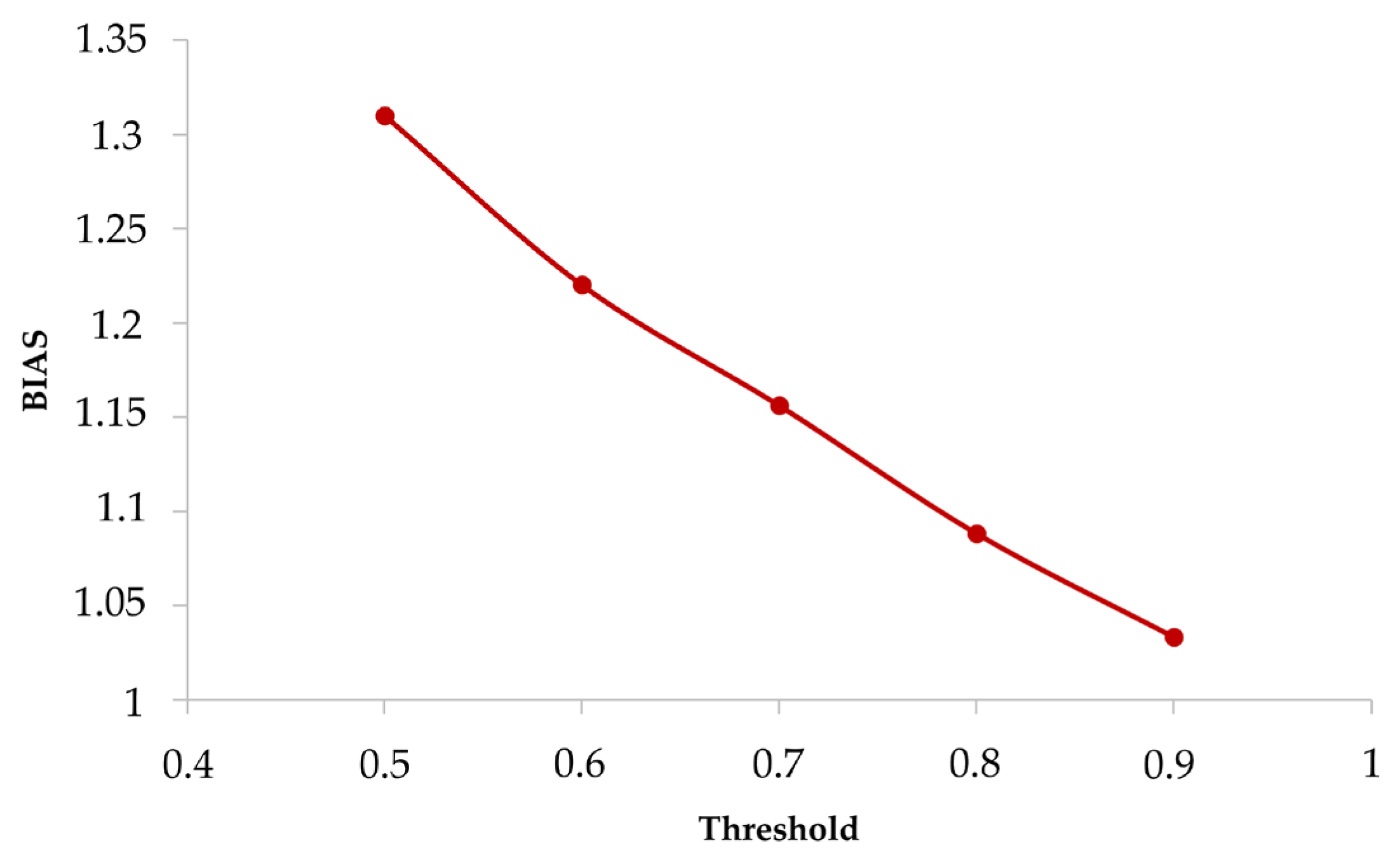
As mentioned before, the threshold for the ECMWF lightning flash density prediction for this study was 0.5 (100 km−2 h−1). For this threshold, the BIAS score was 1.31 for 0.5° resolution. Figure 5 shows the sensitivity of the BIAS values to different lightning flash density thresholds. As the limit increases, the BIAS value decreases, so that for a threshold equal to 0.9 (100 km−2 h−1), the BIAS is approximately 1, showing a perfect BIAS. However, this approximation means that we are losing many forecast values, and the indices (H, TS and ETS) have decreased and worsened their values. For this reason, the value of 0.5 (100 km−2 h−1) was the value chosen for the previous analysis.
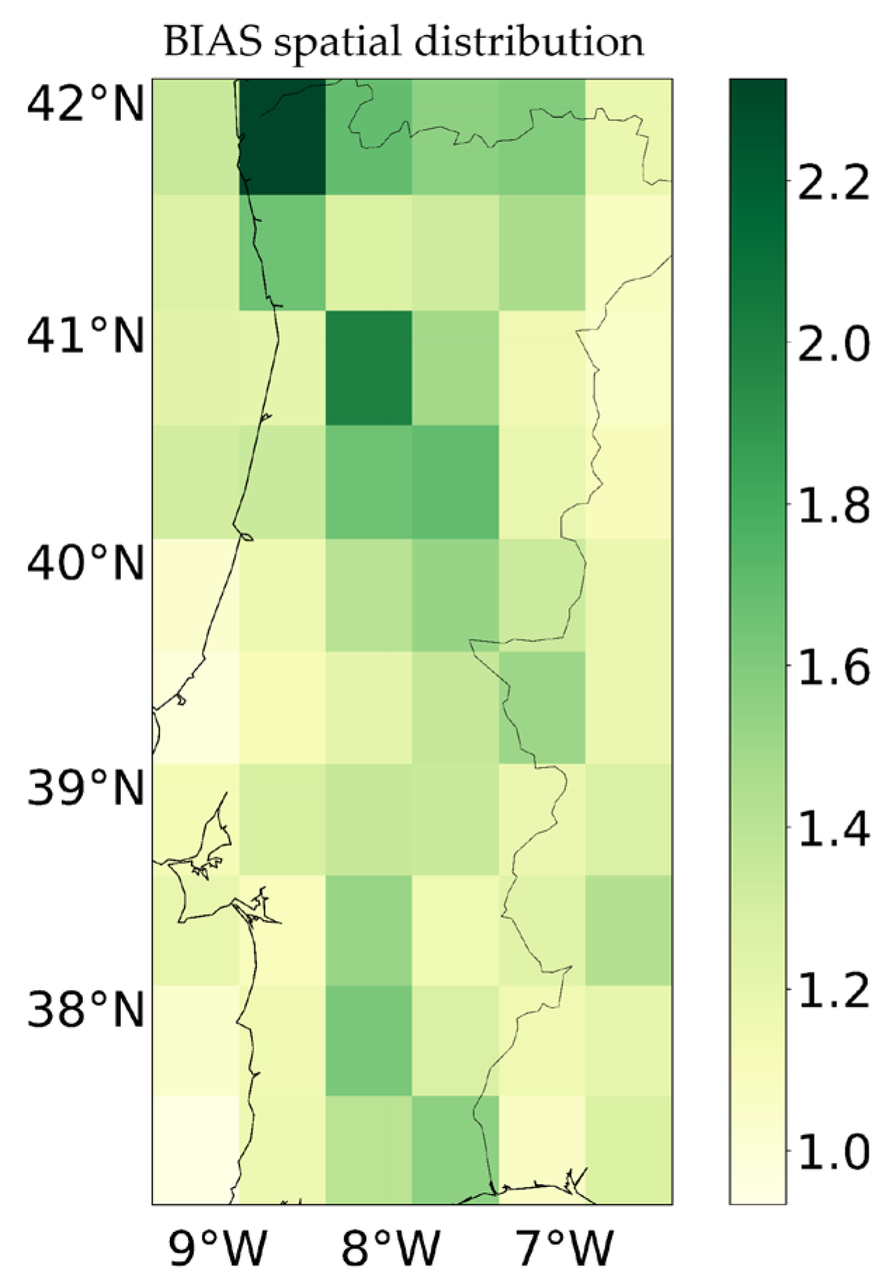
Figure 6 shows the spatial variation of the BIAS score for a 0.5° grid for the period under study. The model overestimates the event number of lightning when compared with observations, with the BIAS score larger than 1 over almost the entire map. It also found two values with the BIAS larger than 2. The figure shows that model had the worst performance in the extreme north of Portugal (dark green).
3.2. Lightning Spatial Distribution and Associated Weather Pattern
To complement the statistical analysis, graphs were drawn for all the cases in which at least 1 of the predicted and/or observed variables were recorded. The synoptic context of events with the highest number of observed or predicted discharges was analyzed. This section discusses three of these cases, representing synoptic situations in which many electrical discharges occurred and/or were predicted.
The first example, on 8 July 2019, is shown in Figure 7 with the lightning concentration in the northeast of Portugal and a good agreement between the total lightning forecast and observation. However, the model predicted lightning activity to begin in the period (0900–1200) UTC (Figure 7a), while they only effectively occur later in the period (1200–1500) UTC (Figure 7b). The highest lightning density predicted by the model occurred at 1500 UTC (with values above 10 (100 km−2 h−1)), but the highest lightning concentration recorded was found for the period (1500–1800) UTC (Figure 7c). In the last figure (Figure 7d), there was no significant lightning density predicted by the model.
This situation suggests a time lag between the model’s lightning prediction and observation, with the model starting and finishing earlier than observed. It is important to highlight that there is a model–observation agreement on the area affected by lightning, i.e., northeast of Portugal.
Figure 8 displays the synoptic situation for the event mentioned above. The geopotential height at 500 hPa on 1800 UTC (Figure 8a) shows the existence of an upper-level low (ULL) centered over the Iberian Peninsula, identified on the geopotential field. It is also shown that the ULL has a cold core (lower temperatures in the center, represented by yellow colors). Figure 8b shows a synoptic chart with the surface pressure and weather fronts in Europe and the Northeast Atlantic, valid at 1800 UTC, on 8 July 2019. The figure shows the presence of the thermal low over the Iberian Peninsula, and an instability line (black line) directed toward the Northeast of Portugal. It should be noted that the ULL is located over the boundary layer thermal low. The presence of an upper low system over the shallow Iberian thermal low enhances the instability and contributed to the increase in convection over the region under study. Therefore, this lightning episode originated from precipitating systems developed under the ULL influence. The synoptic situation described in this example is similar to several other events of high-density electrical discharges, with the only difference being the location of the ULL, which is often to the west of the Peninsula. The radar images displayed in Figure 9a–c show the presence of a convective system over northeastern Portugal, with the main convective cores over Spain, in agreement with the lightning observations (Figure 7).
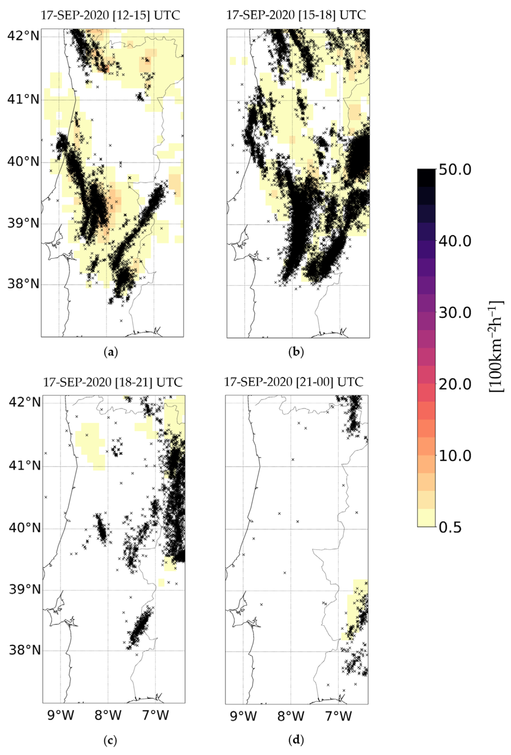
Figure 10 shows the results for a second example, which occurred on 17 September 2020. The model predicted a high density of lightning flashes in the forecast at 1500 UTC and 1800 UTC in the North and Center region (Figure 10a,b).
During this period, the observed data revealed a large lightning concentration in mainland Portugal, also showing good agreement between the predicted and observed data. In this case, the model began to predict a lower density of lightning at 2100 UTC and 0000 UTC forecast, Figure 10c,d, respectively. In the [1800–2100] UTC period, a large lightning concentration is still observed (Figure 10c).
Figure 11 presents the synoptic scale for the region under study between the 17 and 18 September 2020. As in the first example, a low-pressure system is shown in the ECMWF upper-level forecast chart (Figure 11a,c). However, in this case the low system was centered between the archipelagos of Azores and Madeira and moving toward Portuguese territory. In Figure 11b, we can observe the advance of a cold front (blue line) associated with the low-pressure center, with an instability line (black line) advancing through the Iberian Peninsula. As reported in Brown [53], the ULL led to a cut-off low and originated a subtropical storm known as Alpha. The interaction between the upper-level low and a surface front induced the formation of a frontal low, which affected Portugal during days 17 and 18 (Figure 11b,d). This meteorological system made landfall in Portugal in the afternoon of September 18 [53]. Therefore, in this case, the lightning origin was due to the passage of a frontal system, associated with the Alpha storm over Portugal. The radar images from the afternoon of 17 September (Figure 9d–f) highlighted the convective activity in central Portugal, thereby explaining the intense amount of lightning density recorded by the lightning network detection system (Figure 10a–d).
The last example documents a situation in which the ECMWF model failed to correctly predict lightning over the region. As shown in Figure 12, the model predicted lightning over a large domain in the Portugal mainland in the forecast for 1500 UTC (Figure 12a) and 1800 UTC (Figure 11b). However, the observation data only detected a small number of lightning flashes in the 1500–1800 UTC period (Figure 12b). Figure 13 presents the large-scale environment on 1800 UTC, with the geopotential height at 500 hPa (Figure 13a) and the synoptic chart (Figure 13b). Near the surface, the synoptic circulation is similar to the first example, with the development of a shallow thermal low centered over the Iberian Peninsula (Figure 13b). The geopotential height chart at 500 hPa shows an upper-level trough south-west of Iberia (Figure 13a). This configuration of the pressure field at altitude also created conditions of instability but was not as intense or well-defined as the ones in the previous examples. This instability was enough for the model to predict the occurrence of many electrical discharges throughout the country. The radar precipitation rate (Figure 9g–i) shows the development of a very localized convective core in northeastern Portugal, which was the driver of the lightning depicted in Figure 12.
4. Discussion
This study evaluates the ECMWF model performance in predicting lightning occurrence and analyses the lightning spatial distribution patterns during four fire seasons with the respective weather patterns. This study compares with the work developed by Sarkar et al. [43] who also evaluated the ECMWF lightning forecast, comparing it with observation data. The assessment specifically focuses on the 2020 monsoon season in India.
First, a statistical analysis was performed, in which a quantitative comparison was made between the predicted and observed data. Through the construction of matrices of 1° × 1° and 0.5° × 0.5° resolution, two contingency tables were constructed, based on the forecast/occurrence or not (yes/no) of lightnings in each mesh. A sensitivity test was also performed, by changing the lightning flash density threshold considered in order to assume a positive lightning forecast. The results showed that as the threshold increases, the BIAS score improves, while all other statistical indices worsen. Therefore, increasing this threshold would cause the loss of many prediction values, so an appropriate threshold for the area and summer season is 0.5 (100 km−2 h−1). In this study, we assessed the area where the model predicts the occurrence of lightning flashes, but not their intensity, number, or type.
For a 3 h time scale, several statistical indices were calculated described in the literature (e.g., [48]). For both matrices, the value of the BIAS is larger than 1, indicating that the model tends to overpredict the area affected by lightning. The lightning parameterization uses outputs from the IFS convection scheme. Therefore, the results of the parameterization will be influenced by the quality of the IFS forecast outputs. For instance, Bechtold et al. [54] examined the diurnal cycle of convection and precipitation biases with the ECMWF IFS for continental United States and Africa. Their findings revealed that the model tends to bring the forecast forward the diurnal cycle of convection by a few hours. The results also show an underestimated of the occurrence of nocturnal convection. So, these results could potentially impact the calculation of the parameterization used to forecast lightning density.
Sarkar et al. [43] also showed the existence of a BIAS greater than 1, in some cases even greater than 2 and 3. Regarding the 1° resolution analyses, the H values indicate that 0.577 of lightning is correctly predicted, while for a 0.5° resolution, the H is lower (0.49). The F value shows the existence of around 0.027 (0.018) of the occurrences of false predictions of lightning for a spatial resolution of 1° (0.5°). The values found by Sarkar et al. [43] in India show a higher success rate (greater than 80%), but also a higher rate of false alarms. The value of H, found in this study, compares equally well with the verification carried out in Dafis et al. [44] on the use of an explicit lightning forecasting scheme coupled to the WRF model (WRF-E) over Greece, with a finer resolution. Like Sarkar et al. [43], Dafis et al. [44] also found higher values of F. Another study on Greece, also using the WRF model, but using an empirical parameterization algorithm [46], presents higher values for the success rate, but also higher false alarm rate values. As the lightning occurrence is a rare and occasional phenomenon, the majority of “predicted × observed” occurrences will be recorded in the no/no cell, which means that the value of the F index considers all entries in the contingency table, making this value so low. As the true success rate (HK) includes the F index, its value is also influenced.
The value of TS is 0.346 and the ETS is 0.326, when using the 1° resolution grid. These values decrease to 0.269 and 0.258, for the same scores, when assessing the 0.5° resolution data. The ETS values are consistent with those calculated by Dafis et al. [44] and those of Xu et al. [45], both cases referring to the prediction verification with an WRF-E.
Regarding the spatial distribution, the model overestimates the worst in the extreme north of Portugal. One possible reason for this result is the extensive areas of complex terrain in this region.
In terms of weather patterns associated with lightning occurrence, some general aspects are highlighted from the results. In the warmer months, the Iberian Peninsula often experiences low thermal pressure [55]. The development of this system results from surface heating, i.e., the elevated temperatures allow the expansion of heated air producing divergence in altitude. The occurrence of divergence at altitude reduces the pressure at the surface [55]. Hoinka and Castro [55] found the presence of thermal lows over the Iberian Peninsula at 35% to 45% between June and August, highlighting the importance of this phenomenon in the region. The situation presented in this study also showed the predominance of lightning in the northeast of Portugal. Besides the thermal low development, this Portuguese region is characterized by a complex orography that influences the vertical motions, making it easier to trigger convection and the development of precipitating systems. Royé et al. [56] found higher levels of lightning activity in the areas of complex orography in Galiza, Spain. This weather pattern was found in several cases in our analysis. When the boundary layer thermal low was overlapped by an ULL, the convection became deeper and electrical discharges increased. The meteorological situation identified on 8 July 2019, represents this kind of situation. This case from July 2019 is representative of other cases, in which the thermal low was identified near the surface and at altitude an ULL was present, with the difference that the ULL was positioned further west instead of being exactly above the identified thermal low. The presence of this system at altitude has contributed to instability, facilitating the occurrence of convection and consequent formation of lightning.
Another result found is that the period when the lightning concentration is maximum is during the afternoon. In the case of July 2019, for example, the model predicted more lightning density for the 1500 UTC forecast, despite the observed lightning concentration being higher in the following period. This is consistent with the results from Royé et al. [56], which reported that the number of discharges reaches its peak around 1800 UTC, after diurnal heating from solar radiation.
The second weather pattern found favoring lightning occurrence was the passage of frontal systems associated with synoptic-scale cyclones. As shown by Ramos et al. [17], this situation is not common in summer, being more frequent in the winter months. The passage of the Alpha subtropical storm on 17–18 September 2020 [53,57] and its associated cold front over mainland Portugal, led to widespread lightning activity over western Iberia. This was a synoptic-scale weather feature whose evolution was well reproduced by global weather forecasting models. In this event, the good agreement between the forecast and observed data confirmed that the algorithm prediction of lightning, based on model variables, was well adjusted to phenomena on scales well resolved by the model itself. However, on the following day, while still under the influence of the subtropical depression, the weather in mainland Portugal was affected by small scale convergence lines. As these features are more dependent on surface heterogeneities, the forecast and observed lightning data showed a lower agreement.
The third example was associated with a high number of false alarms of lightning occurrence, very clear in the BIAS values, which suggested that the model tends to overpredict lightning occurrence in less unstable synoptic situations. In these cases, the occurrence or inhibition of convection depends on finer-scale phenomena not resolved by the model. The overprediction of the electrical discharges in situations of “intermediate” instability, found in this work and others, suggests the possibility of increasing the value of the thresholds used in the scheme.
These examples agree with Owens [58], who showed that ECMWF’s lightning forecast is not precise in time and space, and therefore it should be interpreted as an overall indicator on a given region. Particularly, the lightning forecast data could show a peak one hour earlier than observed and the activity could drop very quickly in the evening.
5. Conclusions
Given the potential usefulness of ECMWF’s lightning forecast density in a natural forest wildfire research framework, this study evaluated these data in mainland Portugal during four fire seasons. A statistical analysis was conducted, using a dichotomous approach, where all data were aggregated to a resolution of 1° × 1° and 0.5° × 0.5°, and the 3 h forecast was compared with the lightning strikes detected by the national lightning detection network between June and September in the years of 2019 to 2022.
The findings revealed that the model tends to overestimate the lightning occurrence areas. Furthermore, the ECMWF lightning forecast had a true success rate of 0.55 at 1° and 0.48 at 0.5° resolution. However, the results showed a better prediction for southern Portugal. This study also shows that while changing the lightning density threshold required to set the existence of a lightning forecast can improve the BIAS, several other statistical indices worsen as a result. Therefore, the study suggests that a reasonable compromise in mainland Portugal is to consider a threshold of 0.5 (100 km−2 h−1) in the summer season. Although there was a temporal delay between the forecasts and observations, ECMWF’s lightning forecast was able to provide useful guidance on the region where the probability of lightning is large.
The analysis of lightning spatial distribution led us to the identification of some weather patterns associated with lightning activity during the study period. For instance, lightning activity associated with the Iberian thermal low development overlapped by an ULL and the passage of large-scale features such as frontal systems are well reproduced by the model. The study provides insights for the ECMWF lightning forecast applicability in the context of forecasting natural forest fires. Despite achieving positive outcomes, it is important to recognize that the current iteration of the ECMWF has specific limitations that can impact lightning-induced fire forecasts. One notable constraint is the model’s inability to distinguish between CG and CC discharges. This lack of differentiation limits the usefulness of lightning predictions in the context of firefighting, since only CG discharges pose a risk for natural ignition. Additionally, the BIAS value indicates that the model’s tendency to overestimate may lead to false alarms regarding the potential risk of natural ignition. While the tool has proven useful in indicating the days and locations where events are likely to occur, it is essential for authorities to consider other factors such as the region under study, the type of vegetation, and the amount of fuel, which are beyond the scope of this paper. Nevertheless, the results suggest that the model has the potential to assist authorities in assessing the probability of natural ignition events, serving as an additional decision support tool. Then, a more detailed analysis of the precipitating systems producing lightning during the summer season will be addressed in a future study, jointly with the analysis of natural forest fires during the same period. Finally, it is suggested that the time series should be expanded over the entire year, in order to evaluate the model’s sensitivity to interannual variability over Portugal.
Author Contributions
Conceptualization, C.C., F.T.C. and R.S.; methodology, C.C., J.R., F.T.C. and R.S.; software, C.C. and F.L.M.S.; validation, C.C., F.L.M.S., F.T.C., J.R. and R.S.; formal analysis, C.C., F.L.M.S., F.T.C., J.R. and R.S.; investigation, C.C.; resources, R.S., J.R. and T.F.; data curation, C.C. and F.L.M.S.; writing—original draft preparation, C.C.; writing—review and editing, F.L.M.S., J.R., T.F., F.T.C. and R.S.; visualization, C.C. and F.L.M.S.; supervision, F.T.C. and R.S.; project administration, F.T.C. and R.S.; funding acquisition, F.T.C. and R.S. All authors have read and agreed to the published version of the manuscript.
Funding
This research was funded by the European Union through the European Regional Development Fund in the framework of the Interreg V A Spain–Portugal program (POCTEP) through the CILIFO project (Ref.: 0753-CILIFO-5-E) and FIREPOCTEP+ (0139_FIREPOCTEP_MAS_6_E), RH.VITA project (ALT20-05-3559-FSE-000074), and also by national funds through FCT-Foundation for Science and Technology, I.P. under the PyroC.pt project (Ref. PCIF/MPG/0175/2019), ICT project (Refs. UIDB/04683/2020 and UIDP/04683/2020). Filippe Santos was supported by the FCT, I.P with the Grant 2022.11960.BD.
Institutional Review Board Statement
Not applicable.
Informed Consent Statement
Not applicable.
Data Availability Statement
The large-scale meteorological charts and the lightning density data are provided by the European Centre for Medium-Range Weather forecasts (ECMWF). Data can be accessed from the website as long as it is associated with a user: https://www.ecmwf.int/ (accessed on 19 December 2023). The synoptic charts are provided by Met Office, and it can be found at link: https://digital.nmla.metoffice.gov.uk/ (accessed on 19 December 2023). Lightning observations and Radar images are provided by the Portuguese meteorological center (IPMA) and are not publicly available due to the data sharing policy.
Acknowledgments
The authors are grateful to the Portuguese Institute for Sea and Atmosphere (IPMA) for providing lightning and RADAR images of the rainfall rate data, the European Centre for Medium-Range Weather Forecasts (ECMWF) for providing the ECMWF lightning forecast product and meteorological analysis, and the Met Office for the synoptic charts.
Conflicts of Interest
The authors declare no conflicts of interest.
References
- Dupuy, J.; Fargeon, H.; Martin-StPaul, N.; Pimont, F.; Ruffault, J.; Guijarro, M.; Hernando, C.; Madrigal, J.; Fernandes, P. Climate Change Impact on Future Wildfire Danger and Activity in Southern Europe: A Review. Ann. For. Sci. 2020, 77, 35. [Google Scholar] [CrossRef]
- Turco, M.; Rosa-Cánovas, J.J.; Bedia, J.; Jerez, S.; Montávez, J.P.; Llasat, M.C.; Provenzale, A. Exacerbated Fires in Mediterranean Europe due to Anthropogenic Warming Projected with Non-Stationary Climate-Fire Models. Nat. Commun. 2018, 9, 3821. [Google Scholar] [CrossRef] [PubMed]
- Couto, F.T.; Santos, F.L.M.; Campos, C.; Andrade, N.; Purificação, C.; Salgado, R. Is Portugal Starting to Burn All Year Long? The Transboundary Fire in January 2022. Atmosphere 2022, 13, 1677. [Google Scholar] [CrossRef]
- San-Miguel-Ayanz, J.; Durrant, T.; Boca, R.; Maianti, P.; Libertà, G.; Oom, D.; Branco, A.; De Rigo, D.; Ferrari, D.; Roglia, E.; et al. Advance Report on Forest Fires in Europe, Middle East and North Africa 2022; Publications Office of the European Union: Luxembourg, 2023; Available online: https://op.europa.eu/en/publication-detail/-/publication/500b8dfa-de5e-11ed-a05c-01aa75ed71a1/language-en (accessed on 18 December 2023).
- Linley, G.D.; Jolly, C.J.; Doherty, T.S.; Geary, W.L.; Armenteras, D.; Belcher, C.M.; Bird, R.B.; Duane, A.; Fletcher, M.; Giorgis, M.A.; et al. What Do You Mean, “Megafire”? Glob. Ecol. Biogeogr. 2022, 31, 1906–1922. [Google Scholar] [CrossRef]
- Guerreiro, J.; Fonseca, C.; Salgueiro, A.; Fernandes, P.; Lopez Iglésias, E.; de Neufville, R.; Mateus, F.; Castellnou Ribau, M.; Sande Silva, J.; Moura, J.M.; et al. Análise e Apuramento dos Factos Relativos aos Incêndios que Ocorreram em Pedrógão Grande, Castanheira de Pera, Ansião, Alvaiázere, Figueiró dos Vinhos, Arganil, Góis, Penela, Pampilhosa da Serra, Oleiros e Sertã, entre 17 e 24 de junho de 2017—Relatório Final; Comissão Técnica Independente (CTI), Assembleia da República: Lisbon, Portugal, 2017. [Google Scholar]
- Guerreiro, J.; Fonseca, C.; Salgueiro, A.; Fernandes, P.; Lopez Iglésias, E.; de Neufville, R.; Mateus, F.; Castellnou Ribau, M.; Sande Silva, J.; Moura, J.M.; et al. Avaliação dos Incêndios Ocorridos Entre 14 e 16 de outubro de 2017 em Portugal Continental. Relatório Final; Comissão Técnica Independente (CTI); Assembleia da República: Lisbon, Portugal, 2018. [Google Scholar]
- Couto, F.T.; Iakunin, M.; Salgado, R.; Pinto, P.; Viegas, T.; Pinty, J.-P. Lightning Modelling for the Research of Forest Fire Ignition in Portugal. Atmos. Res. 2020, 242, 104993. [Google Scholar] [CrossRef]
- Campos, C.; Couto, F.T.; Filippi, J.-B.; Baggio, R.; Salgado, R. Modelling Pyro-Convection Phenomenon during a Mega-Fire Event in Portugal. Atmos. Res. 2023, 290, 106776. [Google Scholar] [CrossRef]
- Couto, F.T.; Filippi, J.-B.; Baggio, R.; Campos, C.; Salgado, R. Numerical Investigation of the Pedrógão Grande Pyrocumulonimbus Using a Fire to Atmosphere Coupled Model. Atmos. Res. 2024, 299, 107223. [Google Scholar] [CrossRef]
- Sirca, C.; Salis, M.; Arca, B.; Duce, P.; Spano, D. Assessing the Performance of Fire Danger Indexes in a Mediterranean Area. iForest 2018, 11, 563–571. [Google Scholar] [CrossRef]
- Meddour-Sahar, O.; Meddour, R.; Leone, V.; Lovreglio, R.; Derridj, A. Analysis of Forest Fires Causes and Their Motivations in Northern Algeria: The Delphi Method. iForest 2013, 6, 247–254. [Google Scholar] [CrossRef]
- Curt, T.; Borgniet, L.; Bouillon, C. Wildfire Frequency Varies with the Size and Shape of Fuel Types in Southeastern France: Implications for Environmental Management. J. Environ. Manag. 2013, 117, 150–161. [Google Scholar] [CrossRef]
- Bento-Gonçalves, A. Os Incêndios Florestais Em Portugal; Fundação Francisco Manuel dos Santos: Lisbon, Portugal, 2021. [Google Scholar]
- Fernandes, P.M.; Santos, J.A.; Castedo-Dorado, F.; Almeida, R. Fire from the Sky in the Anthropocene. Fire 2021, 4, 13. [Google Scholar] [CrossRef]
- Moreira, N.; Barroso, C.; Bugalho, L.; Correia, S.; Gouveia, C.; Lopes, M.J.; Marques, P.; Pinto, P.; Ramos, R.; Silva, A.; et al. Condições Meteorológicas Relativas ao Incêndio na Lousã em 11 de Julho de 2020; Relatório Interno, IPMA: Lisbon, Portugal, 2020; Available online: https://www.ipma.pt/pt/media/noticias/news.detail.jsp?f=/pt/media/noticias/arquivo/2020/incendiolousa.html (accessed on 19 December 2023).
- Ramos, A.M.; Ramos, R.; Sousa, P.; Trigo, R.M.; Janeira, M.; Prior, V. Cloud to Ground Lightning Activity over Portugal and Its Association with Circulation Weather Types. Atmos. Res. 2011, 101, 84–101. [Google Scholar] [CrossRef]
- Rodrigues, M.; Jiménez-Ruano, A.; Gelabert, P.J.; de Dios, V.R.; Torres, L.; Ribalaygua, J.; Vega-García, C. Modelling the Daily Probability of Lightning-Caused Ignition in the Iberian Peninsula. Int. J. Wildland Fire 2023, 32, 351–362. [Google Scholar] [CrossRef]
- Lopez, P. A Lightning Parameterization for the ECMWF Integrated Forecasting System. Mon. Weather Rev. 2016, 144, 3057–3075. [Google Scholar] [CrossRef]
- Krause, A.; Kloster, S.; Wilkenskjeld, S.; Paeth, H. The Sensitivity of Global Wildfires to Simulated Past, Present, and Future Lightning Frequency. J. Geophys. Res. Biogeosci. 2014, 119, 312–322. [Google Scholar] [CrossRef]
- Brâncuș, M.; Burada, C.; Drîgă, F. The impact of dry thunderstorms in Southwestern Romania. In Proceedings of the 11th European Conference on Severe Storms, Bucharest, Romania, 8–12 May 2023. [Google Scholar] [CrossRef]
- Rorig, M.L.; McKay, S.J.; Ferguson, S.A.; Werth, P. Model-Generated Predictions of Dry Thunderstorm Potential. J. Appl. Meteorol. Climatol. 2007, 46, 605–614. [Google Scholar] [CrossRef]
- Giannaros, T.M.; Papavasileiou, G.; Lagouvardos, K.; Kotroni, V.; Dafis, S.; Karagiannidis, A.; Dragozi, E. Meteorological Analysis of the 2021 Extreme Wildfires in Greece: Lessons Learned and Implications for Early Warning of the Potential for Pyroconvection. Atmosphere 2022, 13, 475. [Google Scholar] [CrossRef]
- Mostajabi, A.; Finney, D.L.; Rubinstein, M.; Rachidi, F. Nowcasting Lightning Occurrence from Commonly Available Meteorological Parameters Using Machine Learning Techniques. NPJ Clim. Atmos. Sci. 2019, 2, 41. [Google Scholar] [CrossRef]
- Blouin, K.D.; Flannigan, M.D.; Wang, X.; Kochtubajda, B. Ensemble Lightning Prediction Models for the Province of Alberta, Canada. Int. J. Wildland Fire 2016, 25, 421–432. [Google Scholar] [CrossRef]
- Lac, C.; Chaboureau, J.-P.; Masson, V.; Pinty, J.-P.; Tulet, P.; Escobar, J.; Leriche, M.; Barthe, C.; Aouizerats, B.; Augros, C.; et al. Overview of the Meso-NH Model Version 5.4 and Its Applications. Geosci. Model Dev. 2018, 11, 1929–1969. [Google Scholar] [CrossRef]
- Barthe, C.; Chong, M.; Pinty, J.-P.; Bovalo, C.; Escobar, J. CELLS V1.0: Updated and Parallelized Version of an Electrical Scheme to Simulate Multiple Electrified Clouds and Flashes over Large Domains. Geosci. Model Dev. 2012, 5, 167–184. [Google Scholar] [CrossRef]
- Skamarock, C.; Klemp, B.; Dudhia, J.; Gill, O.; Liu, Z.; Berner, J.; Wang, W.; Powers, G.; Duda, G.; Barker, D.; et al. A Description of the Advanced Research WRF Model Version 4. In NCAR Technical Note ncar/tn-556+ str; National Center for Atmospheric Research: Boulder, CO, USA, 2019. [Google Scholar] [CrossRef]
- Fierro, A.O.; Mansell, E.R.; MacGorman, D.R.; Ziegler, C.L. The Implementation of an Explicit Charging and Discharge Lightning Scheme within the WRF-ARW Model: Benchmark Simulations of a Continental Squall Line, a Tropical Cyclone, and a Winter Storm. Mon. Weather Rev. 2013, 141, 2390–2415. [Google Scholar] [CrossRef]
- Price, C.; Rind, D. A Simple Lightning Parameterization for Calculating Global Lightning Distributions. J. Geophys. Res. Atmos. 1992, 97, 9919–9933. [Google Scholar] [CrossRef]
- Yair, Y.; Lynn, B.; Price, C.; Kotroni, V.; Lagouvardos, K.; Morin, E.; Mugnai, A.; Llasat, M.D.C. Predicting the Potential for Lightning Activity in Mediterranean Storms Based on the Weather Research and Forecasting (WRF) Model Dynamic and Microphysical Fields. J. Geophys. Res. 2010, 115, D04205. [Google Scholar] [CrossRef]
- McCaul, E.W.; Goodman, S.J.; LaCasse, K.M.; Cecil, D.J. Forecasting Lightning Threat Using Cloud-Resolving Model Simulations. WAF 2009, 24, 709–729. [Google Scholar] [CrossRef]
- Bright, D.R.; Wandishin, M.S.; Jewell, R.E.; Weiss, S.J. A Physically Based Parameter for Lightning Prediction and Its Calibration in Ensemble Forecasts. In Conference on Meteorological Applications of Lightning Data; American Meteorological Society: Boston, MA, USA, 2005. [Google Scholar]
- Federico, S.; Torcasio, R.C.; Lagasio, M.; Lynn, B.H.; Puca, S.; Dietrich, S. A Year-Long Total Lightning Forecast over Italy with a Dynamic Lightning Scheme and WRF. Remote Sens. 2022, 14, 3244. [Google Scholar] [CrossRef]
- Lynn, B.H.; Yair, Y.; Price, C.; Kelman, G.; Clark, A.J. Predicting Cloud-To-Ground and Intracloud Lightning in Weather Forecast Models. WAF 2012, 27, 1470–1488. [Google Scholar] [CrossRef]
- Tsonevsky, I. 45r1 New Parameters: Lightning Flash Density—Forecast User. ECMWF Confluence Wiki. Available online: https://confluence.ecmwf.int/pages/viewpage.action?pageId=106611144 (accessed on 19 December 2023).
- Rio, J. Probabilidade de Ocorrência de Trovoada Seca; Nota Técnica DivMV 08/2020; IPMA: Lisbon, Portugal, 2020. [Google Scholar]
- IPMA. Relatório Condições Meteorológicas Associadas ao Incêndio de Pedrógão Grande de 17 Junho 2017; IPMA: Lisbon, Portugal, 2017; Available online: https://www.ipma.pt/export/sites/ipma/bin/docs/relatorios/meteorologia/20170630-relatorio-pedrogaogrande-ipma-completo.pdf (accessed on 19 December 2023).
- IPMA. Rede de Detetores de Trovoadas no Continente; IPMA: Lisbon, Portugal, 2020; Available online: https://www.ipma.pt/bin/docs/organizacionais/POSEUR-02-1708-FC-000035.pdf (accessed on 19 December 2023).
- Correia, S. Análise de Padrões Temporais e Espaciais de Descargas Elétricas Atmosféricas em Portugal Continental. Master’s Dissertation, University of Lisbon, Lisbon, Portugal, 2012. [Google Scholar]
- Chaudhary, S.; Dhanya, C.T. Expanding Contingency Table for Intensity and Frequency Based “True” Detection of Rainy Events in Precipitation Datasets. Atmos. Res. 2020, 244, 105119. [Google Scholar] [CrossRef]
- Umar, M.; Latif, A.; Mahmood, S.A. Comparative Study of Performance of Real-Time Satellite-Derived Rainfall in Swat Catchment. Arab. J. Geosci. 2017, 10, 126. [Google Scholar] [CrossRef]
- Sarkar, R.; Mukhopadhyay, P.; Bechtold, P.; Lopez, P.; Pawar, S.D.; Chakravarty, K. Evaluation of ECMWF Lightning Flash Forecast over Indian Subcontinent during MAM 2020. Atmosphere 2022, 13, 1520. [Google Scholar] [CrossRef]
- Dafis, S.; Fierro, A.; Giannaros, T.M.; Kotroni, V.; Lagouvardos, K.; Mansell, E. Performance Evaluation of an Explicit Lightning Forecasting System. J. Geophys. Res. Atmos. 2018, 123, 5130–5148. [Google Scholar] [CrossRef]
- Xu, L.; Chen, S.; Yao, W. Evaluation of Lightning Prediction by an Electrification and Discharge Model in Long-Term Forecasting Experiments. Adv. Meteorol. 2022, 2022, e4583030. [Google Scholar] [CrossRef]
- Giannaros, T.M.; Kotroni, V.; Lagouvardos, K. Predicting Lightning Activity in Greece with the Weather Research and Forecasting (WRF) Model. Atmos. Res. 2015, 156, 1–13. [Google Scholar] [CrossRef]
- Giannaros, T.M.; Lagouvardos, K.; Kotroni, V. Performance Evaluation of an Operational Lightning Forecasting System in Europe. Nat. Hazards 2016, 85, 1–18. [Google Scholar] [CrossRef]
- Ebert, E.E. Fuzzy Verification of High-Resolution Gridded Forecasts: A Review and Proposed Framework. Meteorol. Appl. 2008, 15, 51–64. [Google Scholar] [CrossRef]
- Gold, S.; White, E.; Roeder, W.; McAleenan, M.; Kabban, C.S.; Ahner, D. Probabilistic Contingency Tables: An Improvement to Verify Probability Forecasts. WAF 2019, 35, 609–621. [Google Scholar] [CrossRef]
- Met Office’s Website. Digital Library and Archive. Met Office. Available online: https://digital.nmla.metoffice.gov.uk/ (accessed on 19 December 2023).
- ECMWF. Available online: https://www.ecmwf.int/ (accessed on 20 December 2023).
- Instituto Português do Mar e da Atmosfera. IPMA. Available online: https://www.ipma.pt/ (accessed on 19 December 2023).
- Brown, D.P. Subtropical Storm Alpha—Tropical Cyclone Report; NOAA: Washington, DC, USA, 2021. [Google Scholar]
- Bechtold, P.; Semane, N.; Lopez, P.; Chaboureau, J.-P.; Beljaars, A.; Bormann, N. Representing Equilibrium and Nonequilibrium Convection in Large-Scale Models. J. Atmos. Sci. 2014, 71, 734–753. [Google Scholar] [CrossRef]
- Hoinka, K.P.; Castro, M. The Iberian Peninsula Thermal Low. Q. J. R. Meteorol. 2003, 129, 1491–1511. [Google Scholar] [CrossRef]
- Royé, D.; Lorenzo, N.; Martin-Vide, J. Spatial–Temporal Patterns of Cloud-To-Ground Lightning over the Northwest Iberian Peninsula during the Period 2010–2015. Nat. Hazards 2018, 92, 857–884. [Google Scholar] [CrossRef]
- IPMA. Boletim Climatológico de Setembro de 2020; IPMA: Lisbon, Portugal, 2020; Available online: https://www.ipma.pt/pt/publicacoes/boletins.jsp?cmbDep=cli&cmbTema=pcl&cmbAno=2020&idDep=cli&idTema=pcl&curAno=2020 (accessed on 19 December 2023).
- Owens, B. ECMWF Confluence Wiki. Section 8.1.13 Lightning. Available online: https://confluence.ecmwf.int/display/FUG/Section+8.1.13+Lighning (accessed on 19 December 2023).
Figure 1.
Iberian Peninsula. The blue rectangle represents the region under study.

Figure 2.
Interpolation of observational data from IPMA in a regular grid with the same resolution and size as ECMWF grid. (a) Irregular grid: the flash is represented by “×”; (b) Regular grid: the flashes “×” are transformed in a pixel with a horizontal resolution of 0.125°. White pixels represent the location where no flash was detected. The grid size is the same as the ECMWF grid: 41 lines by 25 columns.

Figure 3.
(a) The original size of grid with forecast information that will be reduced to: (b) 1° of horizontal resolution square with information of yes/no, and (c) 0.5° of horizontal resolution squares with information of yes/no. From the original grid with the 41 lines by 25 columns, the grid is reduced to a grid of horizontal resolution of 1° × 1° (0.5° × 0.5°) with 5 (10) lines by 3 (6) columns. The white pixels represented the local where there is no lightning prediction.

Figure 4.
Flow chart summarizing the methodology adopted in the study from the study period choice, aggregation of the forecast, and observation data into a grid with a resolution of 1° and 0.5°, until the statistical analysis.
Figure 4.
Flow chart summarizing the methodology adopted in the study from the study period choice, aggregation of the forecast, and observation data into a grid with a resolution of 1° and 0.5°, until the statistical analysis.

Figure 5.
Relationship between the lightning flash density threshold applied on the ECMWF dataset and the BIAS value corresponding to.
Figure 5.
Relationship between the lightning flash density threshold applied on the ECMWF dataset and the BIAS value corresponding to.

Figure 6.
BIAS spatial distribution over the 0.5° grid for the period under study.

Figure 7.
Case study on 8 July 2019. Averaged total lightning flash density in the last 3 h (shaded, n° 100 km−2 h−1) and data observed (black x) for the same period: (a) 0900 UTC—1200 UTC; (b) 1200 UTC—1500 UTC; (c) 1500 UTC—1800 UTC and (d) 1800 UTC—2100 UTC.
Figure 7.
Case study on 8 July 2019. Averaged total lightning flash density in the last 3 h (shaded, n° 100 km−2 h−1) and data observed (black x) for the same period: (a) 0900 UTC—1200 UTC; (b) 1200 UTC—1500 UTC; (c) 1500 UTC—1800 UTC and (d) 1800 UTC—2100 UTC.

Figure 8.
Large-scale environment on 8 July 2019 at 1800 UTC: (a) geopotential height at 500 hPa (red lines, damgp), wind intensity at 500 hPa (wind barbs, kt), and temperature at 500 hPa (shaded, °C) provided by [51], and (b) mean sea level pressure (black contour, hPa), cold front (blue line), warm front (red line), occluded front (purple line), and troughs (black line) provided by [50].

Figure 9.
RADAR images of the rainfall rate (shaded, mm/h) for Portugal. (a–c) for 19 July 2019; (d–f) for September 17, 2020; (g–i) for 10 June 2022 at the hour indicated at the top of each image. Provided by [52].
Figure 9.
RADAR images of the rainfall rate (shaded, mm/h) for Portugal. (a–c) for 19 July 2019; (d–f) for September 17, 2020; (g–i) for 10 June 2022 at the hour indicated at the top of each image. Provided by [52].


Figure 10.
Case study on 17 September 2020. Averaged total lightning flash density in the last 3 h (shaded, n° 100 km−2 h−1) and data observed (black x) for the same period: (a) 1200 UTC—1500 UTC; (b) 1500 UTC—1800 UTC; (c) 1800 UTC—2100 UTC and (d) 2100 UTC—0000 UTC.
Figure 10.
Case study on 17 September 2020. Averaged total lightning flash density in the last 3 h (shaded, n° 100 km−2 h−1) and data observed (black x) for the same period: (a) 1200 UTC—1500 UTC; (b) 1500 UTC—1800 UTC; (c) 1800 UTC—2100 UTC and (d) 2100 UTC—0000 UTC.

Figure 11.
Large-scale circulation on 17/18 September 2020: (a) geopotential height at 500 hPa (red lines, damgp), wind intensity at 500 hPa (wind barbs, kt), and temperature at 500 hPa (shaded, °C) provided by [51] on 17 September 2020 at 1800 UTC, (b) mean sea level pressure (black contour, hPa), cold front (blue line), warm front (red line), occluded front (purple line), and troughs (black line) provided by [50] and on 17 September 2020 at 1800 UTC, (c) As (a), but on 18 September 2020 at 1800 UTC, and (d) As (b), but on 18 September 2020 at 1800 UTC.

Figure 12.
Case study of 10 June 2022. Averaged total lightning flash density in the last 3 h (shaded, n° 100 km−2 h−1) and data observed (black x) for the same period: (a) 1200 UTC—1500 UTC; (b) 1500 UTC—1800 UTC and (c) 1800 UTC—2100 UTC.
Figure 12.
Case study of 10 June 2022. Averaged total lightning flash density in the last 3 h (shaded, n° 100 km−2 h−1) and data observed (black x) for the same period: (a) 1200 UTC—1500 UTC; (b) 1500 UTC—1800 UTC and (c) 1800 UTC—2100 UTC.

Figure 13.
Large-scale environment on 10 June 2022 at 1800 UTC: (a) geopotential height at 500 hPa (red lines, damgp), wind intensity at 500 hPa (wind barbs, kt) and temperature at 500 hPa (shaded, °C) provided by [51], and (b) mean sea level pressure (black contour, hPa), cold front (blue line), warm front (red line), occluded front (purple line), and troughs (black line) provided by [50].


Table 1.
Example of a contingency table used to compute predictions skill scores: A is the total of hits, B the total of false alarms, C the total of misses, and D the total of correct negatives.
Table 1.
Example of a contingency table used to compute predictions skill scores: A is the total of hits, B the total of false alarms, C the total of misses, and D the total of correct negatives.
| Forecast | Observation | ||
| YES | NO | ||
| YES | A | B | |
| NO | C | D | |
Table 2.
Definition of statistical indices used in the analysis process.
| Statistical Indices | Definition | Description |
|---|---|---|
| BIAS | The frequency bias (BIAS) is the ratio of the number of occurrences predicted (A+B) and the number of observed occurrences (A+C). This parameter reveals if the model is underforecast or overforecast [49]. | |
| Success rate | H is a success rate, calculated as the fraction of observed events that were correctly predicted. | |
| False alarm rate | False alarm rate (F) is calculated as the fraction of false alarms on all non-occurrences. | |
| Threat score | Critical success rate or threat score (TS) is a degree measure of forecast correctness of a given event, calculated as the fraction of correctly predicted events out of all predicted or observed events. This score does not account for correct negatives, so it calculated the fraction of correctly predicted events compared to the observed ones [49]. | |
| Equitable threat score | Equitable threat score (ETS) is calculated as TS but in which a value, Arandom, is subtracted from the numerator and denominator, which represents the correct number predictions of the event occurrence that could be achieved “by luck” only based on knowledge of climatology. Arandom can be calculated by: | |
| True skill score | Hanssen and Kuipper index or true skill score (HK) is a rate of true success, given by the difference between the success rate and the false alarm rate. |
Table 3.
Contingency table for the 1° × 1° based on the ECMWF model (+24 h) for values above 0.5 100 km−2 h−1 and for the observed data for the same period.
Table 3.
Contingency table for the 1° × 1° based on the ECMWF model (+24 h) for values above 0.5 100 km−2 h−1 and for the observed data for the same period.
| Forecast | Observation | ||
| YES | NO | ||
| YES | 1318 | 1529 | |
| NO | 966 | 54,747 | |
Table 4.
Contingency table for the 0.5° × 0.5° based on the ECMWF model (+ 24 h) for values above 0.5 100 km−2 h−1 and for the observed data for the same period.
Table 4.
Contingency table for the 0.5° × 0.5° based on the ECMWF model (+ 24 h) for values above 0.5 100 km−2 h−1 and for the observed data for the same period.
| Forecast | Observation | ||
| YES | NO | ||
| YES | 2501 | 4196 | |
| NO | 2573 | 224,970 | |
Disclaimer/Publisher’s Note: The statements, opinions and data contained in all publications are solely those of the individual author(s) and contributor(s) and not of MDPI and/or the editor(s). MDPI and/or the editor(s) disclaim responsibility for any injury to people or property resulting from any ideas, methods, instructions or products referred to in the content. |
© 2024 by the authors. Licensee MDPI, Basel, Switzerland. This article is an open access article distributed under the terms and conditions of the Creative Commons Attribution (CC BY) license (https://creativecommons.org/licenses/by/4.0/).
Share and Cite
MDPI and ACS Style
Campos, C.; Couto, F.T.; Santos, F.L.M.; Rio, J.; Ferreira, T.; Salgado, R. ECMWF Lightning Forecast in Mainland Portugal during Four Fire Seasons. Atmosphere 2024, 15, 156. https://doi.org/10.3390/atmos15020156
AMA Style
Campos C, Couto FT, Santos FLM, Rio J, Ferreira T, Salgado R. ECMWF Lightning Forecast in Mainland Portugal during Four Fire Seasons. Atmosphere. 2024; 15(2):156. https://doi.org/10.3390/atmos15020156
Chicago/Turabian StyleCampos, Cátia, Flavio T. Couto, Filippe L. M. Santos, João Rio, Teresa Ferreira, and Rui Salgado. 2024. "ECMWF Lightning Forecast in Mainland Portugal during Four Fire Seasons" Atmosphere 15, no. 2: 156. https://doi.org/10.3390/atmos15020156
Note that from the first issue of 2016, this journal uses article numbers instead of page numbers. See further details here.