
Associations between Climate Variability and Livestock Production in Botswana: A Vector Autoregression with Exogenous Variables (VARX) Analysis


1
International Economic Development Program, Graduate School of Humanities and Social Sciences, Hiroshima University, 1-5-1 Kagamiyama, Higashi Hiroshima City 739-8529, Hiroshima, Japan
2
The IDEC Institute, Hiroshima University, 1-5-1 Kagamiyama, Higashi Hiroshima City 739-8529, Hiroshima, Japan
3
Graduate School of Innovation and Practice for Smart Society (SMASO), Hiroshima University, 1-5-1 Kagamiyama, Higashi Hiroshima City 739-8529, Hiroshima, Japan
*
Author to whom correspondence should be addressed.
Atmosphere 2024, 15(3), 363; https://doi.org/10.3390/atmos15030363
Submission received: 30 January 2024
/
Revised: 29 February 2024
/
Accepted: 12 March 2024
/
Published: 16 March 2024
(This article belongs to the Special Issue Influence of Weather Conditions on Agriculture)
Abstract
:The changing climate has a serious bearing on agriculture, particularly livestock production in Botswana. Therefore, studying the relationship between climate and livestock, which at present is largely missing, is necessary for the proper formulation of government policy and interventions. This is critical in promoting the adoption of relevant mitigation strategies by farmers, thereby increasing resilience. The aim of this research is to establish associations between climate variability and livestock production in Botswana at the national level. The paper employs time series data from 1970 to 2020 and the Vector Autoregression with Exogenous Variables (VARX) model for statistical analysis. The trend shows that both cattle and goat populations are decreasing. The VARX model results reveal that cattle and goat populations are negatively associated with increasing maximum temperatures. Cattle respond negatively to increased minimum temperatures as well, while goats tend to respond positively, implying that livestock species react differently to climatic conditions due to their distinct features. The results of the roots of the companion matrix for cattle and goat production meet the stability condition as all the eigenvalues lie inside the unit circle. The study recommends further intervention by the government to deal with increasing temperatures, thereby addressing the dwindling populations of goats and cattle, which have significant contributions to the household economies of smallholders and the national economy, respectively.
1. Introduction
Livestock is an integral part of global agricultural production. According to the Food and Agricultural Organization, the share of livestock in the global value of agricultural output is about 40% [1]. Livestock is a source of livelihood for 1.3 billion people worldwide and also provides 34% of the global food protein [1]. Livestock’s contribution to the overall agricultural output in the Global North and Global South is 40% and 20%, respectively [1]. These figures are likely to grow as the demand for livestock products, particularly meat and dairy, are projected to increase between 2027 and 2050 [2].
Yet, livestock production continues to fall victim to the unrelenting climate shocks. Prolonged droughts, reduced rainfall, floods, and excessive and extremely low temperatures are some of the effects of varying climatic conditions that the livestock sector must contend with. Livestock losses have been recorded in countries prone to climate shocks like Pakistan, Afghanistan, and India, with small stockholders in rural areas being the most affected [3]. Similar trends have also been observed in China [4].
Although the inquiry into the relationship between climate change and livestock has dominated academic and policy discourses since the 2000s, the breakthrough started in the 20th century. From the early 20th century until the 1940s, prominent American ecologist Frederick Clements conducted a series of studies on vegetation and the ecology of the Great Plains and the American West and Southwest [5,6,7,8,9]. Clements argued that the amount of rainfall determines the type of vegetation likely to grow in a particular area [6,7]. Thus, farmers can be informed about the kind of livestock that can be kept. Clements also argued that livestock populations are more likely to be affected by droughts in areas with high rainfall variability. Since then, some academic studies [10,11,12] and several reports from international organizations [13,14,15,16] have been consistent with Clements’ findings.
Global production of cattle and goats is currently affected by severe climate change because the two animal species all over the world are more concentrated in communal systems, particularly in Global South countries where production is largely dictated by rainfall and natural pasture [17]. Several modern studies have shown that cattle and goats usually suffer from heat stress during excessive temperatures [18,19,20,21]. Heat stress is identified as an influential factor since it affects animals in many aspects, often leading to loss of appetite, low food intake, reduced productivity, and low quality of the animal, hence unsatisfactory economic returns for rural poor farmers [4,18]. Heat stress also affects livestock indirectly by compromising the amount of nutrients in plants, which animals depend on for feed, through the process of nutrient leaching [22,23,24,25,26,27]. Some studies have revealed that a rise of 2 °C will negatively impact pasture in regions with arid and semi-arid climates and have positive impacts in humid regions [28]. This means that animals may not acquire the nutrients they need from plants even if they eat the same amount of feed, tempering their physical development [26,28,29].
A variation in climate may also result in livestock water scarcity and low productivity of pastures due to frequent/prolonged drought and reduced rainfall. Water sources dry up while pastures become depleted due to prolonged dry periods and less rainfall [30,31]. However, some studies have shown that goats withstand harsh climatic conditions like high temperatures and drought better than large stock and other small ruminants [20,32,33]. Even under extreme climate conditions, goats are considered worth investing in because they have the potential to transform the lives of the poorest in developing countries, where 90% of the global goat population is concentrated [34]. This could be one of the reasons for the increase in the global goat population, which has more than doubled in the last four decades [34].
Meanwhile, in the Guinea Savannah Ecological zone of Nigeria, and countries like Ethiopia, drought is considered the main climate event that is disruptive to cattle production [35,36]. Kenya is another country prone to climate shocks, as indicated by the Global Climate Risk Index [37]. Consequently, it is observed that livestock production in that country is extremely vulnerable to climate change effects like high temperatures and increased precipitation, hence modest gains in net income for farmers [38,39]. Along these lines, hot temperatures are projected to severely affect net revenue, while an increase in precipitation will positively influence livestock production [4]. In terms of current livestock populations, there are over 1 billion goats and 940 million cattle worldwide [1,40]. The numbers are expected to increase in the future due to a rise in the demand for meat in Global South countries’ urban areas [1]. However, the rate of increase might vary considerably depending on the region and socio-economic factors. Thus, the future of global cattle and goat populations will depend on how climate change is managed and the adoption of sustainable livestock practices.
In Botswana, beef cattle are the dominant livestock followed by goats in terms of stock populations. Beef is Botswana’s only agricultural export to the European Union (EU) and recently to the United Arab Emirates (UAE). It has the largest share of 80% of the agricultural Gross Domestic Product (GDP) [41]. Meanwhile, goats are a valuable resource, particularly for poor small-holder farmers, and contribute towards food security in the country’s rural areas. Goats are the second preferred livestock because they require less effort and can withstand the semi-arid climatic conditions of the country better than other small ruminants [42,43]. The livestock species are also the highest protein source for the poor. Cattle and goat farming follow the commercial and communal systems of farming. The commercial system is still at the infancy stage and prevalent in the west and southwest regions. It is dominated by a few large-scale farmers who can afford private land and the ranching system [44,45,46]. Therefore, the communal system, which is made up of mostly small-holder farmers, accounts for over 90% and 95% of the total cattle and goat populations, respectively [47]. Since the communal system is characterized by free/open-range grazing, it is entirely dependent on natural pasture for livestock feed. This is due to modern feeding technologies being in their infancy stage [44,45,48]. As the communal system is largely rainfed, water scarcity is considered a serious challenge [49,50,51]. This is due to Botswana being a predominantly hot and dry country. As a way of assisting farmers in improving production, the government currently has initiatives such as the Citizenship Entrepreneurial Development Agency (CEDA) and Livestock Management and Infrastructure Development (LIMID) in place.
Despite the importance of livestock in the national economy and the changing climate is a worldwide concern, the literature on climate and agriculture, particularly livestock production in Botswana, is scant. Most studies tend to focus on farmers’ perceptions of climate change and mitigation strategies [52,53,54,55,56]. There are a few notable studies that have examined the relationship between climate and livestock production. Livestock populations in the communal lands of Kgalagadi South (south and south-west Botswana) were found to be increasing with higher mean annual rainfall [57]. The goat population was positively associated with mean annual rainfall, and the relationship was statistically significant. While cattle were also positively associated with mean annual rainfall, the relationship was not statistically significant. Meanwhile, drought was negatively associated with livestock populations. Beef cattle have been found to be very vulnerable to drought [58]. Furthermore, it is projected that the cost of livestock water supply will rise by 23% in the future (2050) due to low rainfall [59]. The shortage of rainfall is likely to contribute negatively to livestock production. Lastly, water scarcity, which is associated with drought and low rainfall, together with other factors like pasture scarcity, predators, theft, pests, and diseases, were found to be a serious challenge for small-stock farmers in the Boteti-Sub District in the Central Region [60]. However, more research on the actual relationship between changing climates and livestock populations at the national level is necessary. Analyzing the relationship between climate and livestock production in semi-arid areas like Botswana is important for proper policy formulation by governments. It also informs livestock farmers on the best mitigation strategies for climate shocks to avoid losses. Therefore, this study aims to (1) establish the kind of associations between climate variability and livestock populations in Botswana and (2) identify climatic variables that may be detrimental to livestock production in Botswana. It uses cattle and goats, which are the dominant livestock species, to determine their relationship with climate variation. In comparison with other studies that use district or household-level data, this study utilizes national-level data.
In addition, the research adds to the limited literature on climate and livestock production in Botswana. The study is divided into three major sections. The introduction is followed by Section 2, which includes explanations of the pre-diagnostic tests of the model. Section 3 is the results and analysis, which is made up of estimations of the model and its post-diagnostic test. Section 4 concludes the results and their discussion.
2. Materials and Methods
2.1. Study Area
The area studied is Botswana. The country is located in Southern Africa. It is bordered by Zambia in the north, Zimbabwe in the northeast, South Africa in the south, and Namibia in the west (Figure 1). The Kalahari Desert, which contains mostly sandy soils, covers two-thirds of the country. The climate pattern is typical of Southern Africa, although rainfall is less compared to neighboring countries. Moreover, rainfall is usually unpredictable, erratic, and very unreliable [49,51,61]. It usually varies from less than 200 mm in the southwest region of the Kgalagadi District to over 650 mm in the Chobe District to the north [49,62].
2.2. Data and Sources
The study employs time series data from 1970 to 2020 sourced from two entities: the World Bank and the Food and Agriculture Organization Statistical Database (FAOSTAT) [63,64]. The data is readily available on the web pages of these two organizations (Table 1) [63,64]. The main variables of interest are cattle production (CP), and goat production (GP), which are the outcome variables. The independent variables are annual agricultural land area (AALA), annual maximum surface air temperature (AMISAT), and annual minimum surface air temperature (AMISAT). AALA, according to the World Bank, is described as the share of land area that is arable, under permanent crops, and permanent pastures. We chose AALA since there is no data for the area of permanent pasture over the years separately. AALA is expected to be positively and significantly associated with natural pasture areas. Therefore, we are interested in AALA, which is land used for five or more years for forage, including natural and cultivated crops. We also introduced binary variables: wet year (WY), which is included in the analysis for CP, and dry year (DY) for GP analysis based on the monthly precipitation data of Botswana from 1951–2020 obtained from the World Bank [63]. The binary variables were created based on whether there was an occurrence of a dry month in a year or not using the Standardized Precipitation Index (SPI), estimated from the monthly precipitation data obtained from the World Bank. The SPI is a statistical indicator for comparing a location’s total precipitation to its long-term rainfall over a given time period. It is mostly preferred in climate variability studies because it analyzes rainfall accurately rather than using average rainfall, which tends to be biased toward higher values [65]. The SPI is more representative than average rainfall [66]. For this study, the dry months are those whose SPI value is -1.00 or less, while those with 1.00 or more are considered wet months. Therefore, any year with a dry month is considered a dry year. The independent variables were chosen based on their direct and indirect relationship with livestock. Table 1 shows the variables, units of measurement, and sources.
2.3. Data Analysis: The VARX Model
The Vector Autoregressive model with Exogenous Variables, (VARX) is used for modeling and predicting the behavior of multiple interdependent variables in time series analysis. It includes two main concepts: Vector Autoregression (VAR) and exogenous variables (X) [67]. The VAR captures the linear dependence of each outcome/dependent variable on its past values (lags) and the past values of other variables in the system, allowing the study of dynamic interactions between the variables [68,69,70]. In this study, CP, GP, and AALA are regarded as endogenous variables because their existence can be altered by national or regional policy. Exogenous variables are not part of the system itself but influence the system and are largely not possible to alter by national or regional policy. Including them in the model allows for analyzing their impact on the system’s dynamics. AMASAT, AMISAT, DY, and WY are exogenous variables since they are not part of the system but can influence the behavior of the endogenous variables. Therefore, the VARX model is suitable for explaining the dynamic behavior of the interaction between the endogenous and exogenous variables or endogenous variables on their own [71]. Some studies in fields that deal with time series data, such as finance, economics, business, political science, and agriculture, commonly employ the VARX model for analysis because it can be used to predict and forecast time series data [71,72]. The following are studies from the mentioned fields that employ the VARX model [73,74,75,76]. The linear form of the VARX model is as follows:
where:
: Outcome (CP or GP) at time t
: The order of the model, indicating the number of lags for endogenous variables
: A vector of exogenous variable at time t
: The order of the model, indicating the number of lags for exogenous variables
, , , : Coefficients of the variables
: Constant
: The vector of the disturbance term
The VARX model specification for this study is as follows:
If p = 3, q = 0
If p = 1, q = 0
where:
: Outcome (CP or GP) at time t
,, : Exogenous variables of AMASAT, AMISAT, and DY/WY
: Constant
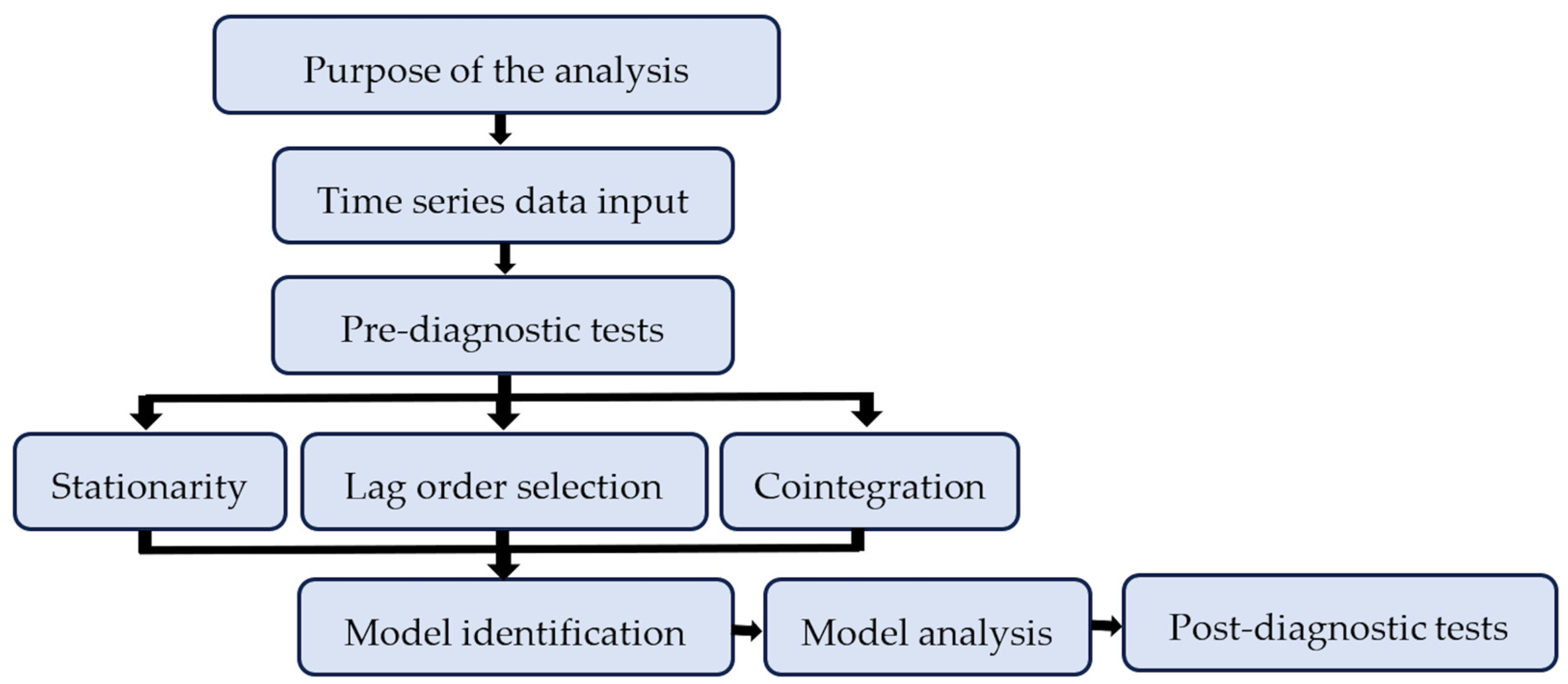
STATA 17 and EViews 13 were used to run the VARX model to complement estimations. The flow of the research is shown in Figure 2.
2.3.1. Pre-Diagnostic Tests
Diagnostic tests such as unit root (stationarity), lag order selection, and cointegration tests are mandatory before running the VARX model.
Unit Root Test
The Augmented Dickey-Fuller (ADF) test was used to determine stationarity and non-stationarity (the presence of a unit root) in the series. If the series are non-stationary, it means that the mean, variance, or covariance are non-constant, implying divergence or convergence of the series with time [77]. The ADF test is preferred for unit root testing due to its ability to account for autocorrelation, control for serial correlation, provide critical values for significance testing, handle different estimation methods, and accommodate trend and intercept terms [78,79]. Some of the drawbacks of the ADF test are that it is sometimes oversized and finds stationarity on many occasions, despite the fact that ADF is the single most widely adopted test for stationarity in time series data [80]. The unit root testing was carried out at the level of the first difference with only an intercept since no trend was detected in the series.
Lag Length Criteria
The lag length of the model needs to be determined before its construction. Through this test, variables from previous years can be included in the model as regressors against the current regression [81]. This boosts model robustness by incorporating dynamic interactions between variables, thereby reducing endogeneity and residual autocorrelation by capturing past shocks. Several tests, like the Likelihood ratio (LR), Final Prediction Error Criterion (FPE), Akaike Information Criteria (AIC), Schwarz Criterion (SC), and Hannan-Quinn Information Criterion (HQ) were used in determining the number of lags for the model.
Cointegration Test
A cointegration test in any VAR model is generally used to ascertain long-run and short-run relationships between the variables [80,82]. The cointegration determines which model must be used based on the long- or short-run relationship. In this study, the Johansen cointegration test was used to determine the cointegration. The test was introduced in 1991 by Johansen to test for cointegration in multivariate time series [83]. Some of the shortfalls of the test, however, are that it is sometimes extremely oversized and tends to imply too many cointegrations [80]. The Johansen cointegration test also has two tests, which are trace and maximum eigenvalue. Both tests seem to have nearly equal strength, as no major differences have been identified between them [84]. However, the trace test tends to be more powerful in some situations. Thus, it is recommended that both tests be applied at the same time, whereas the trace test can be employed exclusively under certain conditions [84].
3. Results and Discussion
3.1. Trends of Cattle and Goat Population
Although the study utilizes data from 1970 to 2020, Figure 3 and Figure 4 present cattle and goat population trends since 1961. For cattle, there was a sharp upward trend from 1966 until 1977, when numbers reached the highest figure ever of 3.1 million. From then on, the population kept fluctuating until it went into a downward mode in 2010. Figure 1 shows that during the five years preceding 2020, the population did not reach 1.5 million, which is approximately half of the highest number ever recorded. This indicates that production has been less satisfactory.
Goat production rose steadily from 1961 to 1970 before dropping the following year. The drop was maintained until 1982. A sharp rise can be observed from 1983 to 1995 when the highest figure of 2.6 million was recorded. However, the drop between 1992 and 1994 should not be overlooked. In summary, the graphs show that production of both livestock species has been going down since 2010, and in 2020, it was still far from the highest numbers ever achieved. While cattle production has been going down for most of the time, goat production was slightly consistent. Perhaps this can be attributed to various factors, amongst them, is climate variation.
3.2. Pre-Diagnostic Tests
3.2.1. Unit Root Test Estimations and Results
The results of the unit root test estimated through the ADF test are illustrated in Table A1. The results indicate that four variables, all exogenous variables, are stationary in level form while three, the endogenous variables, are not. It is further shown that the endogenous variables are stationary at the first-order difference. Therefore, the null hypothesis is rejected for all the variables in the first-order differencing.
3.2.2. Lag Length Criteria
The estimations for the lag length criteria shown in Table A2 and Table A3 indicate that the number of lags selected for cattle production is three and goat production is one. The higher number of lags for cattle production is consistent with the assertion that adding more lags strengthens the model. The results also show that the LR, FPE, AIC, SC, and HQ were responsible for selecting the number of lags, while none was selected by the LL.
3.2.3. Johansen Cointegration Test Estimations
Table A4 and Table A5 show the results of the Johansen Cointegration Test using the Trace and the Maximum Eigenvalue tests for cattle and goat production. For cattle production, the trace test indicates cointegration in only one variable, while the maximum eigenvalue test shows the absence of a long-run relationship among the variables. The results for goat production show cointegration amongst two and one variables for trace and maximum eigenvalue tests, respectively. Therefore, the absence of a long-run relationship between the variables justifies the use of VARX in the study.
3.3. VARX Model Estimations
The model estimations for cattle production in Table 2 show that the coefficient of determination R2 is 0.8953. This suggests that 89.52% of the variation in cattle production is explained by the independent variables. Furthermore, the coefficient of lag 1 of cattle production is positive and significant at a 1% level. This implies that the production of the previous year has a positive influence on the current one. The results indicate that AMASAT and AMISAT are negatively associated with cattle production, as evidenced by the negative coefficients significance levels of 5%. These suggest that the number of cattle tends to decrease with increase in both minimum and maximum temperatures. This negative association can be attributed to heat stress, which have been found to directly affect cattle by retarding their physical development and reproductive ability [85,86,87]. Cattle, especially calves exposed to excessive temperatures, often have weak immunity, which can lead to death [88,89,90]. These findings are also consistent with those of other studies [18]. The results suggest that cattle may be comfortable at average temperatures. This may be possible in ranches where technology is well advanced enough to control temperatures, which may be challenging for the predominant communal system in Botswana. Additionally, with temperatures expected to increase in the future and Botswana being a predominantly hot and dry country, the declining mode of cattle production is likely to persist.
Regarding the variable wet year, the coefficient is also negative and significant at the 5% level. This implies that cattle populations tend to decrease during wetter years. This may also mean that more rainfall is not good for beef cattle. The reason for this could be that wet conditions are a perfect breeding time for parasites such as ticks, tapeworms, wireworms, mites, and liver fluke which often transmit diseases to livestock. Common livestock diseases that occur during the rainy season due to the prevalence of parasites are heartwater, foot rot, and gastrointestinal diseases [91,92]. Gastrointestinal parasites have been found to be largely distributed across small stock and bovine calf species in southern Botswana [93,94]. The downtrend in the cattle population may be abated given that precipitation is projected to decrease in the future in Botswana and other areas of Southern Africa [49,50,63,95,96]. However, this will depend on other factors such as technological advancements, diseases, and feeding techniques. The findings of a negative correlation between cattle production and rainfall conform with some studies [97,98]. The findings are, however, in disagreement with other previous studies [4,57].
The estimations for goat production show that the coefficient of R2 is 0.9175, meaning that the explanatory variables explain 91.75% of the deviation in goat production. Lag 1 for goat production has a high positive coefficient at a 1% significance level, showing that the previous year’s production has a positive influence on the next year’s. This is similar to cattle production, although the coefficients and significance levels are different. The results indicate that goat production also tends to increase with an increase in AALA, and this is significant at 5%. This could mean that the increase in AALA brings more pastures, and thus, plenty of feed for goats, which may boost their reproductive ability. This is also the case with lag 1 of AALA in cattle production, although the results have weak statistical significance. Goat production decreases with an increase in maximum temperatures at the significance level of 1%. Like cattle, this can be connected to heat stress. On the contrary, goat production increases with an increase in minimum temperatures. This can partly be associated with the nature of goats being able to withstand tougher climatic conditions, as established by numerous studies. Lastly, there is a negative association between goat populations and dry years. This may be due to two factors: natural forage and water shortages during dry years, and the findings are similar to those of other studies [57]. The goat population may continue to be in a downward mode if projections of decreased rainfall in the coming years are anything to go by.
3.4. Post-Diagnostic Tests
Tests were also conducted after the model estimation to identify potential model misspecifications and issues like non-normality, autocorrelation or serial correlation, and instability to check the robustness of the model. Those were also conducted to improve the model reliability of the results. The post-diagnostic tests performed were the Granger causality, serial correlation LM, normality tests, and stability. The Granger causality test determines whether one variable can predict the performance of another [99,100], while the Serial correlation LM, also known as the Autocorrelation test, measures the similarity between a time series set and its lagged values [101,102]. The normality test verifies whether a data set is distributed along a normal distribution curve. Results and interpretation may not be reliable if normality has been violated [103,104]. Similarly, VAR models also require stricter stability conditions to be met.
The tests for Serial correlation depicted in Table 3 suggest that there is no autocorrelation among the variables in the selected lag, as evidenced by the probability values that are greater than 0.05. This applies to both cattle and goat production (Table 3).
The findings of the Granger causality test, shown in Table 4, point out some causal relationships between CP and GP and certain variables. There is a bidirectional causal chain connecting CP and AALA. A unidirectional causal chain also exists between CP and AMASAT and CP and WY. In the case of GP, there is only a one-way association between GP and AALA, and GP and AMISAT. All these causalities established by the Granger causality test are also reported in the main estimation (Table 2).
The distribution of observations for cattle and goat production is presented in Figure 5 and Figure 6. The probability values of the normality test results were 3.643 (Jarque-Bera coefficient) with a p-value of 0.16 in the case of cattle production and 2.597 (Jarque-Bera coefficient) with a p-value of 0.27 in the case of goat production confirm that the series is normally distributed.
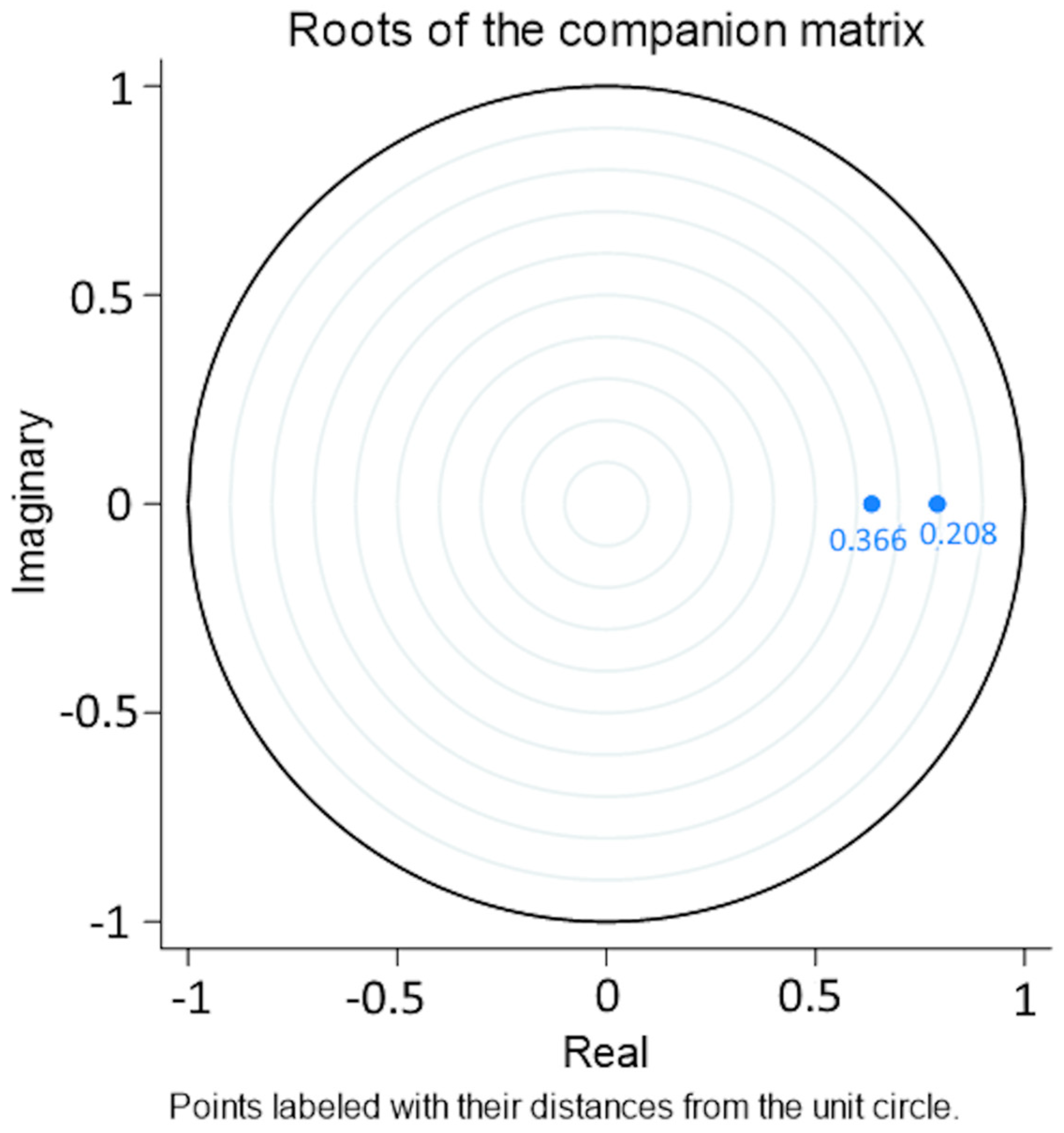
For the stability test, the roots of the companion matrix were used and the results are illustrated in Figure 7 and Figure 8. The figures show that all the eigenvalues lie inside the unit circle, which satisfies the stability condition. Thus, all the results for the post-diagnostic tests point out that the results are robust and reliable.
4. Conclusions
This study has examined the relationship between climate variables and livestock production, namely cattle and goats in Botswana. Cattle and goat populations have been on a downward spiral during the five years preceding 2020. Aside from climate, the downward mode of livestock populations may be due to the failure of government policies in the livestock sector. Results reveal that livestock tend to react similarly to some climatic conditions and differently to others. Both cattle and goats tend to decrease alongside increasing maximum temperatures. This may be due to heat stress which tempers the physical development of animals and weakens the immune system. The trend is likely to continue in the future as temperatures are expected to increase in the future. While cattle react negatively to increase in minimum temperature, goats tend to respond positively. Furthermore, cattle are negatively associated with wet conditions while goats decrease with the occurrence of dry conditions. These show that the animals have distinctive features that make them react and adapt differently to various climatic conditions. The positive relation between goat production and AALA could be an indication that more agricultural land area is needed for pastures or cultivation of goat feed, which could also contribute to cattle production. Lastly, since livestock reacts differently to climatic conditions, the government may consider offering more subsidies for farm equipment and livestock feed to mitigate the effects of predicted increases in temperature and precipitation, specifically for cattle production. Policies like CEDA and LIMID may need to be revisited for easy implementation to ease the capital, management, and infrastructure constraints faced by livestock farmers. This could help livestock farmers ease the challenges posed by climate variability such as increasing temperature and more frequent incidences of intense rain (wet year) or drought (dry year). However, the impacts of such policies on livestock production are yet to be established. Studying the causal impacts of the policies is crucial for their revamping to respond to the actual needs of farmers. Lastly, since this study only establishes correlations there is a need for more quantitative research to establish the actual causal effect of climate variation on livestock production.
Author Contributions
Conceptualization, G.M. and N.P.J.; Methodology, G.M. and N.P.J.; Software, G.M.; Validation, N.P.J.; Formal Analysis, G.M. and N.P.J.; Data Curation, G.M. and N.P.J.; Writing—Original Draft Preparation, G.M.; Writing—Review & Editing, N.P.J.; Visualization, G.M. and N.P.J.; Supervision, N.P.J. All authors have read and agreed to the published version of the manuscript.
Funding
This research received no external funding.
Institutional Review Board Statement
Not applicable.
Informed Consent Statement
Not applicable.
Data Availability Statement
Publicly available datasets were analyzed in this study. This data can be found here https://climateknowledgeportal.worldbank.org/country/botswana, accessed on 29 January 2024 and https://www.fao.org/faostat/en/#data/QCL, accessed on 29 January 2024.
Acknowledgments
The first author (G.M.) expresses deep gratitude to the Government of Japan for providing the MEXT scholarship to pursue a Ph.D. degree at Hiroshima University, Japan. We acknowledge JSPS Grant-in-aid for Scientific Research (KAKENHI)-22K05851 for partially covering the publication fee.
Conflicts of Interest
The authors declare there is no conflict of interest.
Appendix A

Table A1.
ADF unit root test results.
| Variables | T-Statistics at Level | T-Statistics at 1st Difference |
|---|---|---|
| CP | −0.806 | −5.243 *** |
| GP | −1.441 | 7.929 *** |
| AALA | −1.441 | −7.523 *** |
| AMASAT | −5.664 *** | |
| AMISAT | −3.237 ** | |
| WY | −7.207 *** | |
| DY | −8.164 *** |
Notes: ***, and ** represent 1, and 5% significance level.
Table A2.
Lag length criteria for cattle production analysis.
| Lag | LL | LR | FPE | AIC | SC | HQ |
|---|---|---|---|---|---|---|
| 0 | −1037.84 | NA | 7.30 × 10¹⁶ | 44.50 | 44.82 | 44.62 |
| 1 | −990.57 | 82.57 | 1.16 × 10¹⁶ | 42.66 | 43.13 * | 42.84 |
| 2 | −985.40 | 8.58 | 1.11 × 10¹⁶ | 42.61 | 43.24 | 42.85 |
| 3 | −979.34 | 9.55 * | 1.02 × 10¹⁶* | 42.53 * | 43.31 | 42.93 * |
* Indicates lag order selected by the criterion.
Table A3.
Lag length criteria for goat production analysis.
| Lag | LL | LR | FPE | AIC | SC | HQ |
|---|---|---|---|---|---|---|
| 0 | −734.34 | NA | 9.32 × 10¹⁰ | 30.93 | 31.24 | 31.05 |
| 1 | −673.19 | 107.08 * | 8.61 × 10⁹ | 28.55 | 29.02 * | 28.73 * |
| 2 | −670.22 | 4.96 | 9.02 × 10⁹ | 28.59 | 29.22 | 28.83 |
| 3 | −664.88 | 8.45 | 8.59 × 10⁹ * | 28.54 * | 29.32 | 28.83 |
* Indicates lag order selected by the criterion.
Table A4.
Johansen Cointegration Test: Trace and the Maximum Eigenvalue for cattle population.
| Hypothesized No. of CE(s) | Eigenvalue | Trace | Maximum Eigenvalue | ||||
|---|---|---|---|---|---|---|---|
| Statistics | 0.05 CV | Prob. # | Statistics | 0.05 CV | Prob. # | ||
| None | 0.49 | 72.386 | 69.819 | 0.03 ** | 35.022 | 33.877 | 0.077 * |
| At most 1 | 0.333 | 40.110 | 47.856 | 0.219 | 19.057 | 27.584 | 0.410 |
| At most 2 | 0.224 | 21.053 | 29.797 | 0.334 | 12.226 | 21.132 | 0.554 |
| At most 3 | 0.163 | 9.120 | 15.495 | 0.351 | 8.383 | 14.265 | 0.341 |
| At most 4 | 0.015 | 0.736 | 3.841 | 0.391 | 0.736 | 3.841 | 0.391 |
**, * denotes rejection of the hypothesis at 5% and 10% significance level respectively; # MacKinnon –Haug-Michelis (1999) p-values; CV—Critical Value.
Table A5.
Johansen Cointegration Test: Trace and the Maximum Eigenvalue for goat population.
| Hypothesized No. of CE(s) | Eigenvalue | Trace | Maximum Eigenvalue | ||||
|---|---|---|---|---|---|---|---|
| Statistics | 0.05 CV | Prob. # | Statistics | 0.05 CV | Prob. # | ||
| None | 0.573 | 91.482 | 69.819 | 0.00 *** | 41.713 | 33.877 | 0.00 *** |
| At most 1 | 0.408 | 49.769 | 47.856 | 0.03 ** | 25.682 | 27.584 | 0.09 * |
| At most 2 | 0.310 | 24.087 | 29.797 | 0.20 | 18.192 | 21.132 | 0.12 |
| At most 3 | 0.072 | 5.896 | 15.495 | 0.71 | 3.666 | 14.265 | 0.89 |
| At most 4 | 0.044 | 2.230 | 3.841 | 0.14 | 2.230 | 3.841 | 0.14 |
***, **, * denotes rejection of the hypothesis at 1, 5, and 10% significance level respectively; # MacKinnon –Haug-Michelis (1999) p-values; CV—Critical Value.
References
- FAO. World Food and Agriculture—Statistical Yearbook 2022; FAO: Rome, Italy, 2022. [Google Scholar] [CrossRef]
- Peyraud, J.; MacLeod, M. European Commission, Directorate—General, Future of EU Livestock: How to Contribute to a Sustainable Agricultural Sector? Final Report; Publications Office: Luxembourg, 2020; Available online: https://op.europa.eu.en/publication-detail/-/publication/b10852e8.0c33-11eb-bc070laa75ed71a1/language-en (accessed on 20 January 2024).
- Faisal, M.; Abbas, A.; Xia, C.; Raza, M.A.; Akhtar, S.; Ajmal, M.A.; Mushtaq, Z.; Cai, Y. Assessing small livestock herders’ adaptation to climate variability and its impact on livestock losses and poverty. Clim. Risk Manag. 2021, 34, 100358. [Google Scholar] [CrossRef]
- Feng, X.; Qiu, H.; Pan, J.; Tang, J. The impact of climate change on livestock production in pastoral areas of China. Sci. Total Environ. 2021, 770, 144838. [Google Scholar] [CrossRef] [PubMed]
- Clements, F.E. Research Methods in Ecology; University Publishing Co.: Lincoln, NE, USA, 1905. [Google Scholar]
- Clements, F.E. Plant Succession: An Analysis of the Development of Vegetation; Carnegie Institution of Washington: Washington, DC, USA, 1916. [Google Scholar]
- Clements, F.E. Plant Indicators: The Relation of Plant Communities to Process and Practice; Carnegie Institution of Washington: Washington, DC, USA, 1920. [Google Scholar]
- Clements, F.E. Plant Succession and Indicators: A Definitive Edition of Plant Succession and Plant Indicators; Carnegie Institution of Washington, Hafner: Washington, DC, USA, 1928. [Google Scholar]
- Clements, F.E. Dynamics of Vegetation; Allred, B.W., Clements, E.S., Eds.; H. W. Wilson: Bronx, NY, USA, 1949. [Google Scholar]
- Leweri, C.M.; Msuha, M.J.; Treydte, A.C. Rainfall variability and socio-economic constraints on livestock production in the Ngorongoro Conservation Area, Tanzania. SN Appl. Sci. 2021, 3, 123. [Google Scholar] [CrossRef]
- Palmer, P.I.; Wainwright, C.M.; Dong, B.; Maidment, B.I.; Wheller, K.G.; Gedney, N.; Hickman, H.I.; Madani, N.; Folwell, S.S.; Abdo, S.; et al. Drivers and impacts of Eastern African rainfall variability. Nat. Rev. Earth Environ. 2023, 4, 254–270. [Google Scholar] [CrossRef]
- O’Reagain, P.; Bushell, J.; Holloway, C.; Reid, A. Managing for rainfall variability: Effect of grazing strategy on cattle production in a dry tropical savanna. Anim. Prod. Sci. 2009, 49, 85–99. [Google Scholar] [CrossRef]
- UNDP. Agricultural Transformation Model Adapting to Climate Change in the Mekong Delta; UNDP: New York, NY, USA, 2008. [Google Scholar]
- United Nations Development Program (UNDP). Resilient Food and Agriculture; UNDP: New York, NY, USA, 2020. [Google Scholar]
- UNDP. Climate Change Adaptation Project (CCAP) Second Quarter 2016; UNDP: New York, NY, USA, 2016. [Google Scholar]
- World Meteorological Organization (WMO). Statement on the State of the Global Climate; World Meteorological Organization: Geneva, Switzerland, 2018. [Google Scholar]
- Kinda, S.R.; Badolo, F. Does rainfall variability matter for food security in developing countries? Cogent. Econ. Financ. 2019, 7, 1640098. [Google Scholar] [CrossRef]
- Angel, S.P.; Amitha, J.P.; Rashamol, V.P.; Vandana, G.D.; Savitha, S.T. Climate Change and Cattle Production: Impact and Adaptation. J. Vet. Med. Res. 2018, 5, 1134. Available online: https://www.researchgate.net/publication/325333916 (accessed on 3 August 2023).
- Negeri, M.B. The Effects of El Nino on Agricultural GDP of Ethiopia. Am. J. Water Sci. Eng. 2017, 3, 45. [Google Scholar] [CrossRef]
- Joy, A.; Dunshea, F.R.; Leury, B.J.; Clarke, I.J.; Digiacomo, K.; Chauhan, S.S. Resilience of small ruminants to climate change and increased environmental temperature: A review. Animals 2020, 10, 867. [Google Scholar] [CrossRef]
- Sejian, V.; Silpa, M.V.; Reshma Nair, M.R.; Devaraj, C.; Krishan, G.; Bagath, M.; Cauchan, S.S.; Suganthi, R.U.; Fonseca, V.F.C.; Konig, S.; et al. Heat stress and goat welfare: Adaptation and production considerations. Animals 2021, 11, 1021. [Google Scholar] [CrossRef]
- Guo, M.; Liu, J.H.; Ma, X.; Luo, D.X.; Gong, Z.H.; Lu, M.H. The plant heat stress transcription factors (HSFS): Structure, regulation, and function in response to abiotic stresses. Front Plant Sci. 2016, 7, 180954. [Google Scholar] [CrossRef]
- Prasad, P.V.V.; Staggenborg, S.A.; Ristic, Z. Impacts of Drought and/or Heat Stress on Physiological, Developmental, Growth, and Yield Processes of Crop Plants. In Response of Crops to Limited Water: Understanding and Modeling Water Stress Effects on Plant Growth Processes; Ahuja, L.R., Reddy, V.R., Saseendran, S.A., Yu, Q., Eds.; American Society of Agronomy: Madison, WI, USA, 2008; pp. 301–355. [Google Scholar] [CrossRef]
- Zhang, H.; Zhu, J.; Gong, Z.; Zhu, J.K. Abiotic stress responses in plants. Nat. Rev. Genet. 2022, 23, 104–119. [Google Scholar] [CrossRef]
- Thornton, P.K.; van de Steeg, J.; Notenbaert, A.; Herrero, M. The impacts of climate change on livestock and livestock systems in developing countries: A review of what we know and what we need to know. Agric. Syst. 2009, 101, 113–127. [Google Scholar] [CrossRef]
- Sanz-Sáez, Á.; Erice, G.; Aguirreolea, J.; Muñoz, F.; Sánchez-Díaz, M.; Irigoyen, J.J. Alfalfa forage digestibility, quality and yield under future climate change scenarios vary with Sinorhizobium meliloti strain. J. Plant Physiol. 2012, 169, 782–788. [Google Scholar] [CrossRef] [PubMed]
- Polley, H.W.; Briske, D.D.; Morgan, J.A.; Wolter, K.; Bailey, D.W.; Brown, J.R. Climate change and North American rangelands: Trends, projections, and implications. Rangel. Ecol. Manag. 2013, 66, 493–511. [Google Scholar] [CrossRef]
- Rojas-Downing, M.M.; Nejadhashemi, A.P.; Harrigan, T.; Woznicki, S.A. Climate change and livestock: Impacts, adaptation, and mitigation. Clim. Risk Manag. 2017, 16, 145–163. [Google Scholar] [CrossRef]
- Dellar, M.; Topp, C.F.E.; Banos, G.; Wall, E. A meta-analysis on the effects of climate change on the yield and quality of European pastures. Agric. Ecosyst. Environ. 2018, 265, 413–420. [Google Scholar] [CrossRef]
- Akinmoladun, O.F.; Muchenje, V.; Fon, F.N.; Mpendulo, C.T. Small Ruminants: Farmers’ Hope in a World Threatened by Water Scarcity. Animals 2019, 9, 456. [Google Scholar] [CrossRef] [PubMed]
- Akinmoladun, O.F.; Mpendulo, C.T.; Ayoola, M.O. Assessment of the adaptation of Nguni goats to water stress. Animal 2023, 17, 100911. [Google Scholar] [CrossRef] [PubMed]
- Daramola, J.O.; Abioja, M.O.; Iyasere, O.S.; Oke, O.E.; Majekodumni, B.C.; Logunleko, M.O.; Adekunle, E.O.; Nwosu, E.U.; Smith, O.F.; James, I.J.; et al. The resilience of Dwarf goats to environmental stress: A review. Small Rumin. Res. 2021, 205, 106534. [Google Scholar] [CrossRef]
- Koluman, N. Goats and Their Role in Climate Change. Small Rumin. Res. 2023, 228, 107094. [Google Scholar] [CrossRef]
- Utaaker, K.S.; Chaudhary, S.; Kifleyohannes, T.; Robertson, L.J. Global Goat! Is the Expanding Goat Population an Important Reservoir of Cryptosporidium? Front. Vet. Sci. 2021, 8, 648500. [Google Scholar] [CrossRef]
- Ayanlade, A.; Ojebisi, S.M. Climate change impacts on cattle production: Analysis of cattle herders’ climate variability/change adaptation strategies in Nigeria. Change Adapt. Soc.-Ecol. Syst. 2020, 5, 12–23. [Google Scholar] [CrossRef]
- Wako, G.; Tadesse, M.; Angassa, A. Camel management as an adaptive strategy to climate change by pastoralists in southern Ethiopia. Ecol. Process. 2017, 6, 26. [Google Scholar] [CrossRef]
- Sönke, K.; Eckstein, D.; Dorsch, L.; Fischer, L. Global Climate Risk Index 2016: Who Suffers Most from Extreme Weather Events? Weather-Related Loss Events in 2014 and 1995 to 2014; Germanwatch: Bonn, Germany, 2015; ISBN 978-3-943704-04-4. [Google Scholar]
- Kabubo-Mariara, J. The Economic Impact of Global Warming on Livestock Husbandry in Kenya; A Ricardian Analysis. In Proceedings of the African Economic Conference on Globalization, Institutions and Economic Development of Africa, Tunis, Tunisia, 12–14 November 2008; Available online: https://www.afdb.org/fileadmin/uploads/afdb/Documents/Knowledge/30753359-EN-133-KABUBO-MARIARA.PDF (accessed on 15 November 2023).
- Kabubo-Mariara, J. Global warming and livestock husbandry in Kenya: Impacts and adaptations. Ecol. Econ. 2009, 68, 1915–1924. [Google Scholar] [CrossRef]
- Miller, B.A.; Lu, C.D. Current status of global dairy goat production: An overview. Asian-Austral. J. Anim Sci. 2019, 32, 1219–1232. [Google Scholar] [CrossRef]
- International Trade Administration. Agricultural Sectors; International Trade Administration: Washington, DC, USA, 2022. Available online: https://www.trade.gov/country-commercial-guides/botswana-agricultural-sectors (accessed on 6 February 2023).
- Monau, P.I.; Visser, C.; Nsoso, S.J.; Van Marle-Köster, E. A survey analysis of indigenous goat production in communal farming systems of Botswana. Trop. Anim. Health Prod. 2017, 49, 1265–1271. [Google Scholar] [CrossRef] [PubMed]
- Nsoso, S.J.; Monkhei, M.; Tlhwaafalo, B.E. A survey of traditional small stock farmers in Molelopole North, Kweneng district, Botswana: Demographic parameters, market practices and marketing channels. Livest. Res. Rural. Dev. 2004, 16. Available online: http://www.lrrd.org/lrrd16/12/nsos16100.htm (accessed on 6 February 2023).
- Bahta, S.; Temoso, O.; Mekonnen, D.; Malope, P.; Staal, S. Technical efficiency of beef production in agricultural districts of Botswana: A Latent Class Stochastic Frontier Model Approach. In Proceedings of the 30th International Conference of Agricultural Economists, Vancouver, BC, Canada, 28 July–2 August 2018; pp. 1–26. [Google Scholar]
- Ngwako, G. Commercialization and Household Welfare among Smallholder Goat Farmers in Kweneng East Sub-District, Botswana; Egerton University: Egerton-Njoro, Kenya, 2021. [Google Scholar]
- Temoso, O.; Villano, R.; Hadley, D. Evaluating the productivity gap between commercial and traditional beef production systems in Botswana. Agric. Syst. 2016, 149, 30–39. [Google Scholar] [CrossRef]
- Statistics Botswana. Agriculture; Statistics Botswana: Gaborone, Botswana, 2022. [Google Scholar]
- Temoso, O.; Hadley, D.; Villano, R. Performance Measurement of Extensive Beef Cattle Farms in Botswana. Agrekon 2015, 54, 87–112. [Google Scholar] [CrossRef]
- Batisani, N.; Yarnal, B. Rainfall variability and trends in semi-arid Botswana: Implications for climate change adaptation policy. Appl. Geogr. 2010, 30, 483–489. [Google Scholar] [CrossRef]
- Byakatonda, J.; Parida, B.P.; Kenabatho, P.K.; Moalafhi, D.B. Analysis of rainfall and temperature time series to detect long-term climatic trends and variability over semi-arid Botswana. J. Earth Syst. Sci. 2018, 127, 25. [Google Scholar] [CrossRef]
- Statistics Botswana. Botswana Environment Statistics Climate Digest; Statistics Botswana: Gaborone, Botswana, 2019; Available online: www.statsbots.org.bw (accessed on 17 January 2024).
- Akinyemi, F.O. Climate Change and Variability in Semiarid Palapye, Eastern Botswana: An Assessment from Smallholder Farmers’ Perspective. Am. Meteorol. Soc. 2017, 9, 349–364. [Google Scholar] [CrossRef]
- Bosekeng, L.C.; Mogotsi, K.; Bosekeng, G. Farmers’ perception of climate change and variability in the North-East District of Botswana. Livest Res. Rural Dev. 2020, 32, 17. Available online: https://www.researchgate.net/publication/338571027 (accessed on 11 September 2023).
- Juana, J.; Makepe, P.; Kahaka, Z.; Juana, J.S.; Okurut, F.N.; Makepe, P.M. Climate change perceptions and adaptations for livestock farmers in Botswana. Int. J. Econ. Issues 2016, 9, 1–21. Available online: https://www.researchgate.net/publication/307931501 (accessed on 15 December 2023).
- Mogomotsi, P.K.; Sekelemani, A.; Mogomotsi, G.E.J. Climate change adaptation strategies of small-scale farmers in Ngamiland East, Botswana. Clim. Change 2020, 159, 441–460. [Google Scholar] [CrossRef]
- Mugari, E.; Masundire, H.; Bolaane, M. Adapting to climate change in semi-arid rural areas: A case of the Limpopo basin part of Botswana. Sustainability 2020, 12, 8292. [Google Scholar] [CrossRef]
- Kgosikoma, O.E.; Batisani, N. Livestock population dynamics and pastoral communities’ adaptation to rainfall variability in communal lands of Kgalagadi South, Botswana. Pastoralism 2014, 4, 19. [Google Scholar] [CrossRef]
- Masike, S.; Urich, P. Vulnerability of Traditional Beef Sector to Drought and the Challenges of Climate Change: The Case of Kgatleng District, Botswana; University of Botswana: Gaborone, Botswana, 2008; Volume 1, Available online: http://www.academicjournals.org/JGRP (accessed on 7 November 2023).
- Masike, S.; Urich, P. The Projected Cost of Climate Change to Livestock Water Supply and Implications in Kgatleng District, Botswana. World J. Agric. Sci. 2009, 5, 597–603. [Google Scholar]
- Binge, A.; Mshenga, P.; Kgosikoma, K. Production and marketing constraints of small stock farming: Evidence from LIMID and non-LIMID farmers in Boteti Sub-District, Botswana. J. Agribus. Rural. Dev. 2019, 3, 195–201. [Google Scholar] [CrossRef]
- Tsheko, R. Rainfall reliability, drought and flood vulnerability in Botswana. Water SA 2003, 29, 389–392. [Google Scholar] [CrossRef]
- Kashe, K.; Mogobe, O.; Kolawole, O.D. Dryland crop production in Botswana: Constraints and opportunities for smallholder arable farmers. In Smallholder Farmers and Farming Practices: Challenges and Prospects; Kolawole, T., Ed.; Nova Science Publishers: Hauppauge, NY, USA, 2019; pp. 1–34. Available online: https://www.researchgate.net/publication/338212708 (accessed on 12 January 2024).
- World Bank. Climate Change Overview: Country Summary—Botswana. 2023. Available online: https://climateknowledgeportal.worldbank.org/country/botswana (accessed on 22 April 2023).
- FAOSTAT. Crops and Livestock Products. Available online: https://www.fao.org/faostat/en/#data/QCL (accessed on 14 April 2023).
- National Weather Service. Standardized Precipitation Index. Available online: https://www.weather.gov/hfospi_info (accessed on 25 June 2023).
- National Drought Mitigation Center. SPI Generator [Software]. University of Nebraska-Licoln. Published 2018. Available online: https://drought.unl.edu/Monitoring/SPI/SPIProgram.aspx (accessed on 24 June 2023).
- Ocampo-Díaz, S.; Rodríguez-Niño, N. An Introductory Review of a Structural VAR-X Estimation and Applications. Borradores Econ. 2011, 3, 479–508. [Google Scholar] [CrossRef]
- Sims, C.A. Macroeconomics and Reality. Econom. Soc. 1980, 48, 1–48. [Google Scholar] [CrossRef]
- Sun, S.; Lu, H.; Tsui, K.L.; Wang, S. Nonlinear vector auto-regression neural network for forecasting air passenger flow. J. Air Trans. Manag. 2019, 78, 54–62. [Google Scholar] [CrossRef]
- Wooldridge, J.M. Introductory Econometrics: A Modern Approach, 3rd ed.; Thomson South-Western: Mason, OH, USA, 2006. [Google Scholar]
- Warsono, R.E.; Wamiliana, W.; Usman, M. Vector autoregressive with exogenous variable model and its application in modeling and forecasting energy data: Case study of PTBA and HRUM energy. Int. J. Energy Econ. Policy 2019, 9, 390–398. [Google Scholar] [CrossRef]
- Nicholson, W.B.; Matteson, D.S.; Bien, J. VARX-L: Structured Regularization for Large Vector Autoregressions with Exogenous Variables. Int. J. Forecast. 2017, 33, 627–651. [Google Scholar] [CrossRef]
- Brooks, C.; Tsolacos, S. Forecasting models of retail rents. Environ Plan A. 2000, 32, 1825–1839. [Google Scholar] [CrossRef]
- Cushman, D.O.; Zha, T. Identifying monetary policy in a small open economy under flexible exchange rates. J. Monet. Econ. 1997, 39, 433–448. [Google Scholar] [CrossRef]
- Nijs, V.R.; Srinivasan, S.; Pauwels, K. Retail-price drivers and retailer profits. Mark. Sci. 2007, 26, 473–487. [Google Scholar] [CrossRef]
- Wood, B.D. Presidential saber rattling and the economy. Am. J. Pol. Sci. 2009, 53, 695–709. [Google Scholar] [CrossRef]
- Fingleton, B. Spurious spatial regression: Some Monte Carlo results with a spatial unit root and spatial cointegration. J. Reg. Sci. 1999, 39, 1–19. [Google Scholar] [CrossRef]
- Li, G.; Qin, S.J.; Yuan, T. Nonstationarity and Cointegration Tests for Fault Detection of Dynamic Processes. IFAC Proc. Vol. 2014, 49, 10616–10621. [Google Scholar] [CrossRef]
- Warsame, A.A.; Sheik-Ali, I.A.; Hassan, A.A.; Sarkodie, S.A. Extreme climatic effects hamper livestock production in Somalia. Environ Sci. Pollut. Res. 2021, 29, 40755–40767. [Google Scholar] [CrossRef] [PubMed]
- Gianfreda, A.; Maranzano, P.; Parisio, L.; Pelagatti, M. Testing for integration and cointegration when time series are observed with noise. Econ. Model 2023, 125, 106352. [Google Scholar] [CrossRef]
- Agbenyo, S. The Effect of Mental Rehearsal and Imagery on Music Performance Anxiety among Junior High School Students. J. Adv. Res. Multidiscip. Stud. 2022, 2, 1–8. [Google Scholar] [CrossRef]
- Granger, C.W.J. Time Series Analysis, Cointegration, and Applications. Am. Econ. Rev. 2004, 94, 421–425. [Google Scholar] [CrossRef]
- Johansen, S. Estimation and Hypothesis Testing of Cointegration Vectors in Gaussian Vector Autoregressive Models. Econometrica 1991, 59, 1551–1580. [Google Scholar] [CrossRef]
- Lütkepohl, H.; Saikkonen, P.; Trenkler, C. Maximum eigenvalue versus trace tests for the cointegrating rank of a VAR process. Econom. J. 2001, 4, 287–310. [Google Scholar] [CrossRef]
- Wang, S.; Li, Q.; Peng, J.; Niu, H. Effects of Long-Term Cold Stress on Growth Performance, Behavior, Physiological Parameters, and Energy Metabolism in Growing Beef Cattle. Animals 2023, 13, 1619. [Google Scholar] [CrossRef]
- Brown-Brandl, T.M. Understanding heat stress in beef cattle. Brazilian J. Anim. Sci. 2018, 47, e20160414. [Google Scholar] [CrossRef]
- Bunning, H.; Wall, E. The effects of weather on beef carcass and growth traits. Animal 2022, 16, 100657. [Google Scholar] [CrossRef]
- Godde, C.M.; Mason-D’Croz, D.; Mayberry, D.E.; Thornton, P.K.; Herrero, M. Impacts of climate change on the livestock food supply chain; a review of the evidence. Glob. Food Sec. 2021, 28, 100488. [Google Scholar] [CrossRef] [PubMed]
- Dahl, G.E.; Tao, S.; Laporta, J. Heat Stress Impacts Immune Status in Cows across the Life Cycle. Front Vet. Sci. 2020, 7, 116. [Google Scholar] [CrossRef]
- Fu, X.; Zhang, Y.; Zhang, Y.G.; Yin, L.Y.; Yan, S.C.; Zhao, Y.Z.; Shez, W.V. Research and application of a new multilevel fuzzy comprehensive evaluation method for cold stress in dairy cows. J. Dairy Sci. 2022, 105, 9137–9161. [Google Scholar] [CrossRef]
- Eygelaar, D.; Jori, F.; Mokopasetso, M.; Sibeko, K.P.; Collins, N.E.; Vorster, I. Tick-borne haemoparasites in African buffalo (Syncerus caffer) from two wildlife areas in Northern Botswana. Parasites Vectors 2015, 8, 26. [Google Scholar] [CrossRef]
- Gunathilaka, N.; Niroshana, D.; Amarasinghe, D.; Udayanga, L. Prevalence of Gastrointestinal Parasitic Infections and Assessment of Deworming Program among Cattle and Buffaloes in Gampaha District, Sri Lanka. Biomed. Res. Int. 2018, 2018, 3048373. [Google Scholar] [CrossRef] [PubMed]
- Sharma, S.; Busang, M. Prevalence of some gastrointestinal parasites of ruminants in southern Botswana. Botswana J. Agric. Appl. Sci. 2013, 9, 97–103. [Google Scholar]
- Johansson, T. Gastrointestinal Nematodes in Goats in Small Holder Flocks around Gaborone, Botswana; Swedish University of Agricultural Sciences: Uppsala, Sweden, 2017. [Google Scholar]
- Samuel, S.; Dosio, A.; Mphale, K.; Faka, D.N.; Wiston, M. Comparison of multi-model ensembles of global and regional climate model projections for daily characteristics of precipitation over four major river basins in southern Africa. Part II: Future changes under 1.5 °C, 2.0 °C and 3.0 °C warming levels. Atmos. Res. 2023, 293, 106921. [Google Scholar] [CrossRef]
- Dosio, A.; Jones, R.G.; Jack, C.; Lennard, C.; Nikulin, G.; Hewitson, B. What can we know about future precipitation in Africa? Robustness, significance and added value of projections from a large ensemble of regional climate models. Clim. Dyn. 2019, 53, 5833–5858. [Google Scholar] [CrossRef]
- Afonso, N. Impact of Rainfall on East Coast Fever in Cattle at Ol Pejeta; Swedish University of Agricultural Sciences: Uppsala, Sweden, 2022. [Google Scholar]
- Chepkwony, R.; Castagna, C.; Heitkönig, I.; Van Bommel, S.; Van Langevelde, F. Associations between monthly rainfall and mortality in cattle due to East Coast fever, anaplasmosis and babesiosis. Parasitology 2020, 147, 1743–1751. [Google Scholar] [CrossRef]
- Rossi, B.; Wang, Y. Vector autoregressive-based Granger causality test in the presence of instabilities. Stata. J. 2019, 19, 883–899. [Google Scholar] [CrossRef]
- Shojaie, A.; Fox, E.B. Granger Causality: A Review and Recent Advances. Annu. Rev. Stat. Appl. 2022, 9, 289–319. [Google Scholar] [CrossRef] [PubMed]
- Abdulhafedh, A. How to Detect and Remove Temporal Autocorrelation in Vehicular Crash Data. J. Trans. Technol. 2017, 7, 133–147. [Google Scholar] [CrossRef]
- Martin, I. On the Autocorrelation of the Stock Market. J. Financ. Econom. 2021, 19, 39–52. [Google Scholar] [CrossRef]
- Hernandez, H. Testing for Normality: What is the Best Method? ForsChem Res. Rep. 2021, 6, 1–38. [Google Scholar] [CrossRef]
- Khatun, N. Applications of Normality Test in Statistical Analysis. Open J. Stat. 2021, 11, 113–122. [Google Scholar] [CrossRef]
Figure 1.
Map of Africa, Botswana (Source: UN Geospatial https://www.un.org/geospatial/content/botswana accessed on 29 January 2024).
Figure 1.
Map of Africa, Botswana (Source: UN Geospatial https://www.un.org/geospatial/content/botswana accessed on 29 January 2024).

Figure 2.
Research flowchart.

Figure 3.
Cattle population trends, 1961–2020 (FAOSTAT, 2022).

Figure 4.
Goat population trends, 1961–2020 (FAOSTAT, 2022).

Figure 5.
Normality test results for cattle production.

Figure 6.
Normality test results for goat production.

Figure 7.
Roots of the companion for Cattle production.

Figure 8.
Roots of the companion for Goat production.

Table 1.
List of variables and data sources.
| Variable | Abbreviation | Measurement | Data Source |
|---|---|---|---|
| Cattle Production | CP | Annual number of live animals | FAOSTAT |
| Goat Production | GP | Annual number of live animals | FAOSTAT |
| Annual Agricultural Land Area | AALA | Square kilometers (sq2 km) | World Bank |
| Annual Maximum Surface Air Temperature | AMASAT | Degrees Celsius (°C) | World Bank |
| Annual Minimum Surface Air Temperature | AMISAT | Degrees Celsius (°C) | World Bank |
| Dry year (SPI value < −1) | DY | DY Dummy (1—Yes, 0—Otherwise) | Author’s computation |
| Wet year (SPI value > 1) | WY | WY Dummy (1—Yes, 0—Otherwise) | Author’s computation |
Table 2.
Model estimation for cattle and goat production.
| Variables | Cattle Production (CP) | Goat Production (GP) | ||||
|---|---|---|---|---|---|---|
| Coefficient | Std. Err. | p-Value | Coefficient | Std. Err. | p-Value | |
| CP L1 | 1.147 | 0.140 | 0.00 *** | |||
| CP L2 | −0.309 | 0.206 | 0.13 | |||
| CP L3 | 0.042 | 0.134 | 0.75 | |||
| GP L1 | 0.886 | 0.048 | 0.00 *** | |||
| AALA L1 | 93.697 | 58.230 | 0.11 | 0.088 | 0.044 | 0.05 ** |
| AALA L2 | −113.877 | 60.717 | 0.06 * | |||
| AALA L3 | −23.789 | 55.783 | 0.67 | |||
| AMISAT | −167,364.9 | 82,533.9 | 0.04 ** | 309.889 | 73.688 | 0.00 *** |
| AMASAT | −44,806.8 | 22,429.7 | 0.05 ** | −102.965 | 20.609 | 0.00 *** |
| WY | −131,144.4 | 65,697.9 | 0.05 ** | |||
| DY | −203.386 | 73.421 | 0.01 *** | |||
| _cons | 15,300,000 | 13,300,000 | 0.25 | −23,749.9 | 12,140.42 | 0.05 ** |
| R-squared | 0.8953 | 0.9175 | ||||
Notes: ***, ** and * represent 1, 5, and 10% significant level.
Table 3.
Autocorrelation LM test for cattle and goat production.
| Lag | Cattle Production | Goat Production | ||||||
|---|---|---|---|---|---|---|---|---|
| LRE * Stat | Df | Rao F-Stat | p-Value | LRE * Stat | Df | Rao F-Stat | p-Value | |
| 1 | 5.41 | 4 | 1.385 | 0.24 | 2.88 | 4 | 0.724 | 0.58 |
| 2 | 0.18 | 4 | 0.044 | 0.99 | ||||
| 3 | 5.06 | 4 | 1.293 | 0.28 | ||||
* Edgeworth expansion corrected likelihood ratio statistic; Df—degree of freedom.
Table 4.
Granger causality tests.
| Variables | Granger Causality | F-Statistics | p-Value | Direction of Causality |
|---|---|---|---|---|
| Cattle production (Lag 3) | AALA does not Granger Cause CP | 2.922 | 0.05 ** | Bidirectional |
| CP does not Granger Cause AALA | 3.196 | 0.03 ** | ||
| AMASAT does not Granger Cause CP | 2.547 | 0.07 * | Unidirectional | |
| CP does not Granger Cause AMASAT | 0.981 | 0.41 | ||
| AMISAT does not Granger Cause CP | 1.850 | 0.15 | No causality | |
| CP does not Granger Cause AMISAT | 1.996 | 0.13 | ||
| WY does not Granger Cause CP | 2.546 | 0.07 * | Unidirectional | |
| CP does not Granger Cause WY | 1.534 | 0.22 | ||
| Goat production (Lag 1) | AALA does not Granger Cause GP | 6.393 | 0.05 ** | Unidirectional |
| GP does not Granger Cause AALA | 0.933 | 0.34 | ||
| AMASAT does not Granger Cause GP | 0.758 | 0.39 | No causality | |
| GP does not Granger Cause AMASAT | 1.608 | 0.21 | ||
| AMISAT does not Granger Cause GP | 2.636 | 0.10 * | Unidirectional | |
| GP does not Granger Cause AMISAT | 0.058 | 0.13 | ||
| DY does not Granger Cause GP | 0.003 | 0.96 | No causality | |
| GP does not Granger Cause DY | 0.019 | 0.89 |
Notes: ** and * represent 1, 5, and 10% significant level.
Disclaimer/Publisher’s Note: The statements, opinions and data contained in all publications are solely those of the individual author(s) and contributor(s) and not of MDPI and/or the editor(s). MDPI and/or the editor(s) disclaim responsibility for any injury to people or property resulting from any ideas, methods, instructions or products referred to in the content. |
© 2024 by the authors. Licensee MDPI, Basel, Switzerland. This article is an open access article distributed under the terms and conditions of the Creative Commons Attribution (CC BY) license (https://creativecommons.org/licenses/by/4.0/).
Share and Cite
MDPI and ACS Style
Matopote, G.; Joshi, N.P. Associations between Climate Variability and Livestock Production in Botswana: A Vector Autoregression with Exogenous Variables (VARX) Analysis. Atmosphere 2024, 15, 363. https://doi.org/10.3390/atmos15030363
AMA Style
Matopote G, Joshi NP. Associations between Climate Variability and Livestock Production in Botswana: A Vector Autoregression with Exogenous Variables (VARX) Analysis. Atmosphere. 2024; 15(3):363. https://doi.org/10.3390/atmos15030363
Chicago/Turabian StyleMatopote, Given, and Niraj Prakash Joshi. 2024. "Associations between Climate Variability and Livestock Production in Botswana: A Vector Autoregression with Exogenous Variables (VARX) Analysis" Atmosphere 15, no. 3: 363. https://doi.org/10.3390/atmos15030363
Note that from the first issue of 2016, this journal uses article numbers instead of page numbers. See further details here.