
High-Resolution Temperature Evolution Maps of Bangladesh via Data-Driven Learning

1
Climate Modeling Laboratory, School of Mathematics, Shandong University, Jinan 250100, China
2
Department of Mathematics, University of Chittagong, Chittagong 4331, Bangladesh
3
Wolfson College, Oxford University, Oxford OX2 6UD, UK
4
Institute of Biomedical and Environmental Science and Technology, University of Bedfordshire, Luton LU1 3JU, UK
*
Author to whom correspondence should be addressed.
Atmosphere 2024, 15(3), 385; https://doi.org/10.3390/atmos15030385
Submission received: 5 February 2024
/
Revised: 11 March 2024
/
Accepted: 15 March 2024
/
Published: 21 March 2024
(This article belongs to the Section Atmospheric Techniques, Instruments, and Modeling)
Abstract
:As a developing country with an agricultural economy as a pillar, Bangladesh is highly vulnerable to adverse effects of climate change, so the generation of high-resolution temperature maps is of great value for Bangladesh to achieve agricultural sustainable development. However, Bangladesh’s weak economy and sparse meteorological stations make it difficult to obtain such maps. In this study, by mining internal features and links inside observed data, we developed an efficient data-driven downscaling technique to generate high spatial-resolution temperature distribution maps of Bangladesh directly from observed temperature data at 34 meteorological stations with irregular distribution. Based on these high-resolution historical temperature maps, we further explored a data-driven forecast technique to generate high-resolution temperature maps of Bangladesh for the period 2025–2035. Since the proposed techniques are very low-cost and fully mine internal links inside irregular-distributed observations, they can support relevant departments of Bangladesh to formulate policies to mitigate and adapt to climate change in a timely manner.
1. Introduction
Global warming is one of the largest threats facing human society, with an increase of ~0.99 °C in mean temperature compared with those in the pre-industrial period, and the mean temperature is predicted to rise further by 1–3 °C by the end of the 21st century [1]. As a result, the increased severity and frequency of floods, hailstorms, droughts, changes in precipitation, and other disaster events have significant impacts on the livelihood capacity of residents especially in developing countries [2,3]. Bangladesh is a poor developing country with an agrarian economy located in the subtropical region of South Asia, and it is often hit by various natural disasters, including but not limited to floods, hurricanes, and droughts, and its agricultural production is extremely vulnerable to climate disasters. Currently, Bangladesh is listed as the seventh most affected country in the world by climate change according to the Global Climate Risk Index 2020 [4], so there is an urgent need for high-resolution climate information to understand patterns and behaviors of climate change and then assess related risks and develop suitable mitigation strategies. However, the sparse and irregular distribution of meteorological stations in Bangladesh is far from enough to achieve this aim.
The emergence of statistical downscaling techniques has increased the possibility of obtaining high-resolution spatial data from low-resolution data [5,6]. Two-dimensional interpolation is the first tool used to downscale coarse-scale climate observation, but it ignores the impacts of topographic factors on climate, resulting in tat the obtained climate maps often containing unrealistic parallel structures [7]. In order to overcome this limitation, the mature statistical downscaling model (SDSM) software uses multiple linear regression to convert the output of large-scale and low-resolution GCM outputs into small-scale and high-resolution regional climate information [8,9]. The SDSM is the most widely used mature tool for regional climate downscaling and forecasting [10,11]. However, large-scale atmospheric circulation always affects regional climate through a complex nonlinear process, so although the SDSM uses a large number of GCM outputs, the downscaling performance by SDSM with multiple linear regressions is not satisfactory [12], especially Han et al. [13] found that after inputting more than 20 large-scale atmospheric circulation factors, the accuracy of SDSM for downscaling temperature and precipitation in Bangladesh is still poor. The quantile mapping was developed to correct for any deviations in GCM simulation and downscaling process [14,15,16], but this approach is highly dependent on the resolution of reanalysis data (e.g., NCEP gridded data with a resolution of 2.5° × 2.5°), leading to this difficult to produce high-resolution downscaled data. Alamgir et al. [14] developed a prognostic statistical downscaling approach for Bangladesh by using CMIP5 outputs under future scenarios, but this approach is only suitable for gridded data and is computationally intensive. Therefore, the widely-used statistical downscaling techniques have limitations to meet high accuracy and high spatial resolution requirements.
Compared with statistical downscaling techniques, advanced data-driven learning techniques have shown excellent performance in handling complex nonlinear correlations between factors [17]. Data-driven learning is used to establish various models through mining internal features and links inside observed data [18]. Mainstream data-driven learning techniques include: the Support Vector Machine (SVM), which uses kernel functions to map complex data features into high-dimensional spaces in order to achieve the aim of accuracy prediction; Random Forest (RF) uses bagging or bootstrap aggregation to combine a series of small-scale decision trees for obtaining better prediction than that by any single tree; Gradient Boosting Regressor (GBR) is an ensemble regression tree, where a new tree is added to fit residuals and then reduce losses, finally obtaining higher prediction accuracy; the extreme gradient boosting (XGBoost) is an ensemble of gradient boosting decision trees. XGBoost supports parallel computing, leading to great improvements in the model training speed. These data-driven learning techniques have a wide range of applications in the field of environment and climate change. Zhang et al. [19] used random forest to predict soil organic carbon in an intensively managed reclamation zone of eastern China. Li et al. [20] compared the prediction effects of SVM and RF in icing severity. Nguyen et al. [21] used RF models to predict the Normalized Difference Vegetation Index values to study the potential impact of climate change on vegetation growth. Trinh et al. [22] used Logistic regression, SVM, and RF to generate landslide susceptibility mapping in the Ha Giang province of Vietnam. Eltazarov et al. [23] used RF to downscale gridded precipitation data and then investigate the risk reduction potential of weather index insurance. Zhang et al. [24] developed a data-driven wind turbine fault detection technique with the help of XGBoost. Li et al. [25] proposed the use of the XGBoost model to quickly evaluate the severity of aircraft icing under different flight conditions.
Due to backward socio-economic development and its flat plain with low altitude, Bangladesh is widely recognized as one of the countries most affected by climate change. At the same time, Bangladesh has only very limited observations from irregularly distributed meteorological stations. In order to make reasonable planning to fight or mitigate the adverse effects of climate change and achieve agricultural sustainable development, Bangladesh urgently needs maps of high-resolution climate evolutions. Unfortunately, traditional climate modeling depending on high running costs and a huge amount of input parameters from observations cannot be utilized by poor Bangladesh. In this study, we developed a low-cost data-driven downscaling technique to generate finer spatially resolved temperature distribution maps for Bangladesh. After that, we explored the data-driven technique to generate a high-resolution temperature forecast map for 2025–2035. This whole article was organized as follows: Section 2 describes climate and environmental conditions in Bangladesh and the sources of climate and topographic datasets used. Section 3 introduces the structure and features of the main data-driven learning models. Section 4 develops the data-driven downscaling technique and generates high-resolution temperature distribution maps of Bangladesh. Section 5 explores the data-driven forecasting technique and generates high-resolution temperature forecast maps of Bangladesh. Finally, Section 6 gives the conclusions and some discussion of the study.
2. Study Area and Data
Bangladesh is in the northeastern part of the South Asian subcontinent and is located in the alluvial delta of the Ganges and Brahmaputra rivers, bordering India on the east, west, and north, Myanmar to the southeast, and the Bay of Bengal to the south. Bangladesh is flat, the main terrain consists of floodplains and delta plains, with only some highlands in the north). Most of the country has a subtropical monsoonal climate, consisting of four seasons: winter (December to February), pre-monsoon summer (March to May), rainy season (June to September) and post-monsoon autumn (October to November) [26]. The mean annual temperature in Bangladesh ranges from 25 to 30 °C, with winter being the most pleasant season of the year with a minimum temperature of 4 °C, and with summer highs usually ranging from 38 °C to about 41 °C, with April being the hottest month and January being the coldest. More than 80% of the precipitation occurs during the rainy season, with an average relative humidity of 80% and an annual precipitation of about 2428 mm, ranging from 1900 mm in the north-west and south-west regions to 3100 mm in the north-east region [27].
The aim of our study is to develop a low-computation-cost and quick downscaling/forecast technique. Since Bangladesh has only limited irregular-distribution meteorological stations and limited computing resources, Bangladesh urgently needs such a downscaling/forecast technique. However, many environmental impact factors are poorly observed in Bangladesh, while topographic factors in Bangladesh are the only available factors observed in a high-resolution manner. At the same time, it is well-known that topographic factors have large impacts on temperature, e.g., a place with a high altitude has a low temperature; a place with a higher latitude has a low temperature. Therefore, we choose three topographic factors to support the generation of high-resolution temperature maps in Bangladesh.
Meteorological stations in Bangladesh are sparsely distributed and uneven (Figure 1). The daily temperature data from 1989–2018 were collected from 34 meteorological stations of the Bangladesh Meteorological Department, and the longitude, latitude, and altitude data were extracted from the Global Multi-resolution Terrain Elevation Data 2010 (Table 1) (https://doi.org/10.5066/F7J38R2N, assessed at 1 December 2023). These data were used to generate high-resolution temperature distribution/forecast maps in Section 4 and Section 5.
3. Data-Driven Learning Models
Compared with statistical downscaling techniques, advanced statistical learning techniques have shown excellent performance in handling complex nonlinear correlations between variables [18]. We used support vector machine (SVM), random forest (RF), gradient boosted regression (GBR), and eXtreme Gradient Boosting (XGBoost).
Support vector machine (SVM) is a non-parametric kernel-based supervised statistical learning model used to solve non-linear regression issues [28]. SVM maps the input vectors into a high dimensional feature space using some nonlinear kernel functions and applies an optimum linear hyper-plane to separate data. For given training data , the SVM finds a regression function such that has at most deviation from the actual value , where denotes a nonlinear transformation from -dimensional space to a higher dimensional feature space, is a weighting matrix, and is a bias term. By minimizing the following regression risk:
subject to . where is a cost function and is a constant which determines the tradeoff between minimizing training errors and minimizing the model complexity term .
Random forest (RF) is an extension of regression trees (CART) to improve prediction accuracy. It combines the output of multiple decision trees to reach a single result [29,30]. Every tree is generated from a random vector that is sampled independently and has the same distribution for all trees in the forest. The divisions within each tree are determined by a subset of predictor variables randomly selected from all existing predictors. When the random forest model is applied for regression, the final output is the average of the results of all trees. In the random forest model, the number of trees in the forest (), the number of variables used to grow each tree (), and the minimum number of per terminal nodes (nodesize) are the main parameters that affect the performance of random forest. The reliable estimates of the errors can be calculated by Out-of-Bag (OOB) data, which are a random subset of data that are not involved in the tree-building process. The mean square error () can be calculated:
where is the number of observations, is the measured value of the variable, and is the average of all OOB predictions.
Gradient boosting regressor (GBR) is an ensemble learning algorithm that uses a boosting technique to minimize the loss of the model by adding weak learners in a stage-wise fashion. In each iterative step, a “weak” regression tree is fitted on a negative gradient (to reduce the loss) of the given loss function and added to the model. The final GBR output is the ensemble of all the regression trees [31]. GBR is the application of gradient boosting and involves three elements: a loss function (which needs to be optimized), a weak learner (used for making predictions), and an additive model (to add weak learners to minimize the loss function). The main goal of this algorithm is to construct the new base-learners to be maximally correlated with the negative gradient of the loss function. Consider an additive model of this form [32]:
where are the basis functions, which are also called weak learners of boosting. Gradient boosting regressor builds the additive model in a forward stage-wise fashion:
At each stage, choosing the decision tree to minimize the loss function , given the current model , and its fitting .
The initial model is problem-specific; for least-squares regression, we chose the mean of the target values. For any given differentiable loss function , we started from an initial model, such as . then iterating until convergence was reached.
eXtreme gradient boosting (XGBoost) is an optimized-distributed gradient boosting library designed to be highly efficient, flexible, and portable [33]. XGBoost is fundamentally the same as GBR since both of them are based on gradient-boosting implementations. Unlike GBR, XGBoost does regularization of the tree as well avoiding overfitting and it also deals with missing values efficiently.
4. High-Resolution Temperature Distribution Maps
We developed efficient downscaling models to generate high spatial-resolution temperature distribution maps, where the daily temperature data and longitude/latitude/altitude of the station were used as inputs to the statistical learning model. The output is a downscaled temperature product. Our downscaling model can largely compensate for the shortcomings of the multilinear-regression-based downscaling techniques (e.g., statistical downscaling models (SDSMs).
To demonstrate the accuracy and efficiency of our models with traditional MLR downscaling models, we generated high spatial-resolution temperature distribution maps directly from daily temperatures observed at 34 meteorological stations with irregular distribution. The correlation of determination (R2), mean absolute error (), and root mean square error () were used to assess the performance of different downscaling models. We adopted the 5-fold cross-validation [34] in fairly comparing model performance. The main process during model training was to randomly divide all stations into five subsets. Each time, we took data on one subset of stations as the test set and data on the remaining four subsets of stations as the training set. The validation process was repeated five times and we finally took the average of five errors to measure model performance. All parameters of the model are automatically chosen by Scikit-Learn [35]. Since the size of training data is not large, the proposed techniques can run very quickly on a regular laptop with the 12th Gen Intel® Core™ i5-12500H.
Based on the daily temperature data and latitude/longitude/altitude data of Bangladesh from 1989 to 2018, we built downscaling models based on SVM, RF, and GBR algorithms, respectively, to obtain higher-resolution temperature data. Table 2 compares the validation results of the three statistical learning downscaling models and one MLR downscaling model in simulating daily mean temperature values. Through 5-fold cross-validation, the downscaled temperatures obtained by the GBR were in best agreement with the original data, followed by RF and SVM, but all were significantly better than the traditional MLR model. The MLR can only extract the linear relationship between topographic factors and temperature variables, leading to that the accuracy by MLR being the worst. The GBR downscaling model produced the highest (0.98) and the lowest (0.06) and (0.08). Figure 2 shows the correlation between the downscaled temperature values and station-wise observations, where the GBR downscaled model fitted the best, followed by the RF, and the SVM with relatively poor results. A Taylor diagram is a visualization tool that compares the performance of different models by simultaneously displaying the correlation coefficients, standard deviations, and root mean square errors among multiple model simulations and station observations. Figure 3 shows a Taylor diagram with observed and simulated temperature data. Clearly, GBR has the best performance of any of the three remaining models, RF and SVM have similar accuracy, and MLR has the poorest performance.
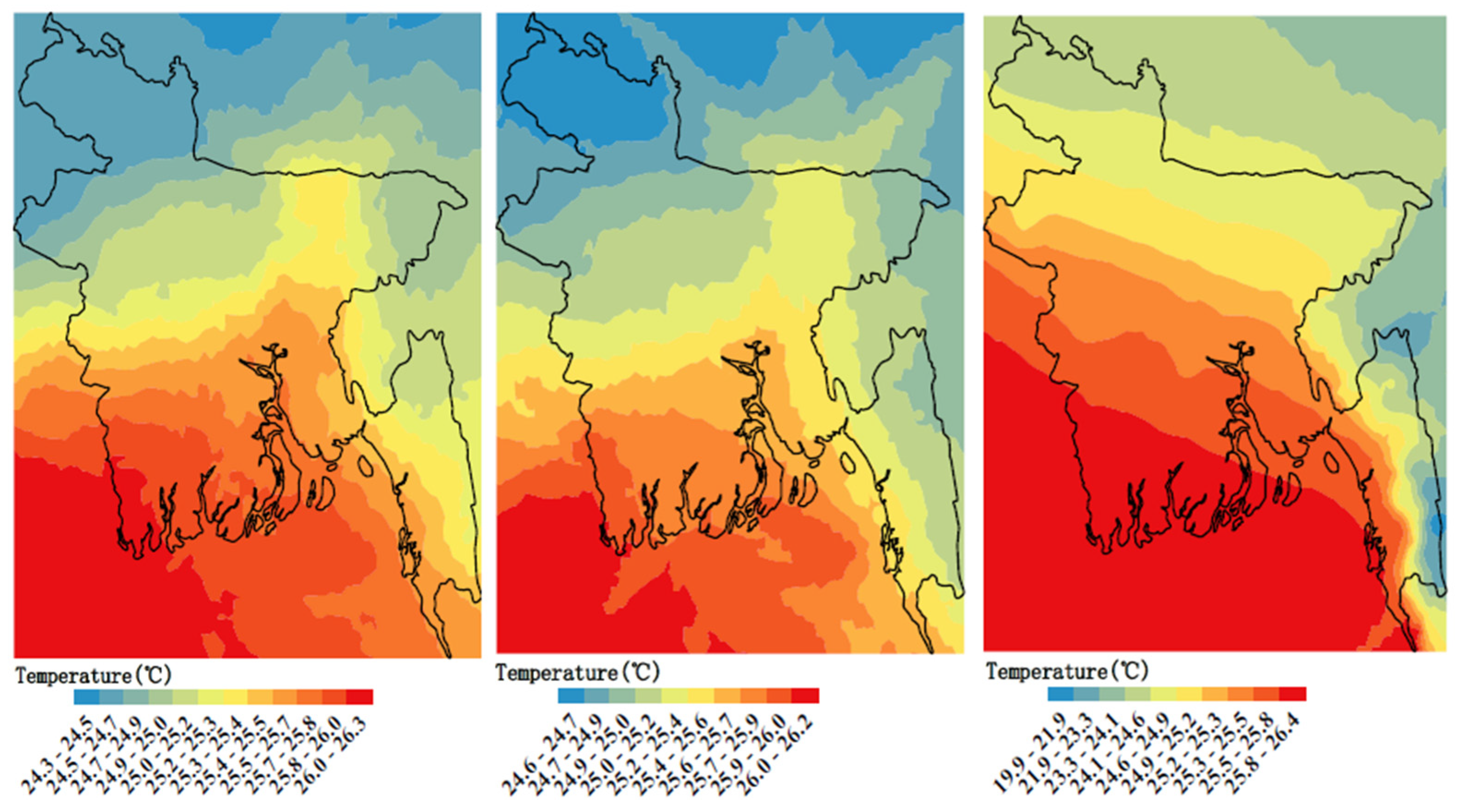
High-resolution mean annual temperature distribution maps are shown in Figure 4. Two maps generated by GBR and RF are basically consistent, while the map by RF contained unrealistic parallel structures. Combining this with Table 2, it means that the GBR downscaled model generated the high-resolution temperature distribution map with the best accuracy. From Figure 4-left the mean annual temperature distribution of Bangladesh had relatively small regional variations, ranging from 24.3 °C to 26.3 °C. The temperature values gradually increased from the northeast to the southwest, reaching the highest in the southwest region.
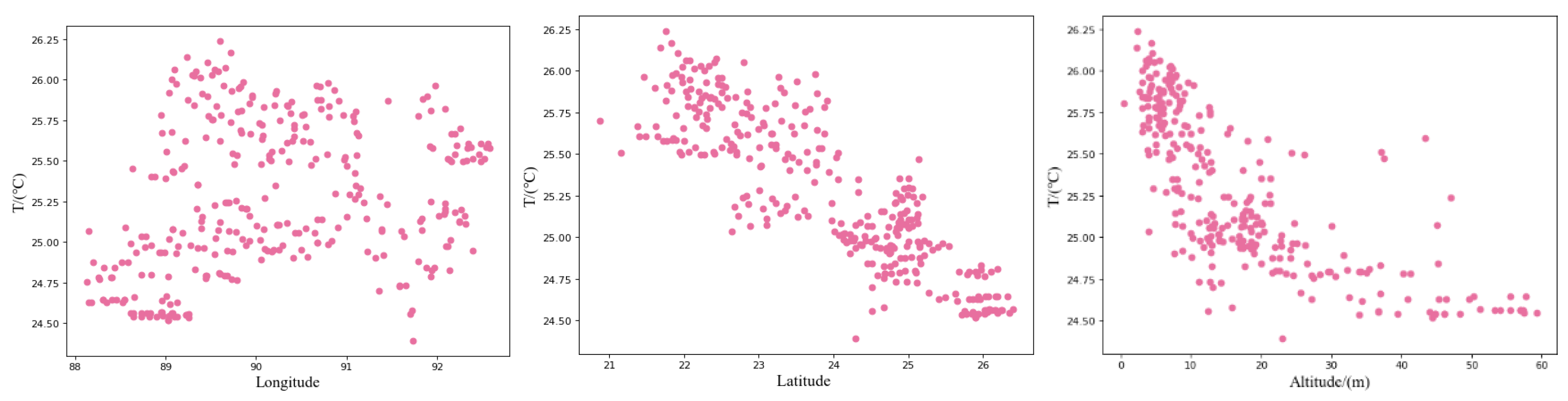
We further make a feature significance analysis of topographic factors (longitude, latitude, and altitude) for the spatial distribution of mean annual temperatures in Bangladesh (Figure 5). It is very clear that latitude and altitude are closely linked with temperature. With the increasing latitude and altitude, the mean annual temperature demonstrates a significantly decreasing trend. However, longitude is not particularly linked with temperature.
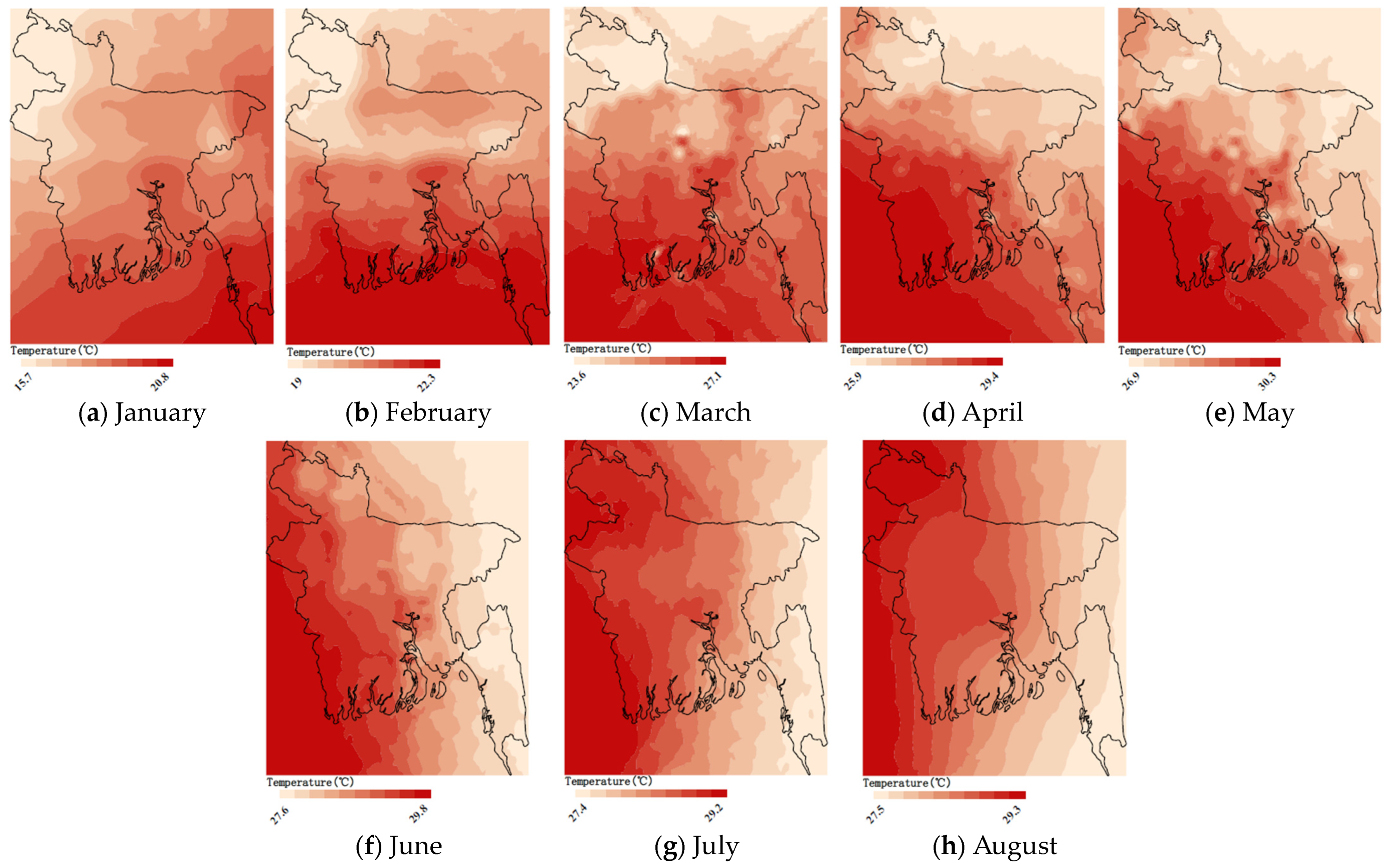
As the monthly variation in Bangladesh temperature is large, Figure 6 shows the high-resolution monthly temperature distribution maps generated by the GBR downscaling model. It reveals a significant seasonal variation in the monthly mean temperature in Bangladesh, with the lowest monthly mean temperature of 15.7 °C (January) and the highest monthly mean temperature of 30.3 °C (May). The spatial patterns of mean temperatures during January–March (or October–December) are similar, with a gradual increase in temperature from the north to the south, peaking in coastal regions, and an overall cooler temperature in the northwestern region. In both April and May, high monthly temperatures are concentrated in the southwestern region, the central region spans a wide range of temperatures, and the northern, eastern, and southeastern regions have relatively low temperatures. The average temperatures in June–August gradually decrease from the west to the east, with a significant increase in the northern region compared with May. The variation of temperatures is relatively small in September, with a difference of no more than 1 °C in each region. Bangladesh demonstrates significant regional variations in the mean monthly temperatures.
5. High-Resolution Temperature Forecast Maps
Accurate climate prediction is of great value for Bangladesh to develop suitable plans for the mitigation of climate disasters and achieve sustainable development. Due to the high dimensionality, complexity, and uncertainty of the climate system, it is difficult to obtain good forecasts for future climate evolution. The known climate forecasts by CMIP6 models must depend on a huge amount of input parameters and high computing resources. Bangladesh does not have enough observations, computing resources, and financial support to run CMIP6 models. Moreover, the resolution of the CMIP6 model is just 1–2 degrees. In this study, we try to explore the low-cost data-driven climate forecast with high resolution (about 0.1 degrees) directly from limited climate observations. The forecast scenario adopted in this study is the “business as usual” scenario. Since the temperature forecast by CMIP6 models is based on RCP-SSP scenarios, we cannot compare our forecast with the low-resolution CMIP6 forecast.
As a set of gradient boosting decision trees, the XGBoost has a fast-training speed and high accuracy when dealing with complex nonlinear links and effectively avoids overfitting problems [36,37]. In this section, we use the XGBoost model to predict future temperature distribution under the business as usual (BAU) climate scenario. The input of the XGBoost model is the high-resolution downscaled historical temperature data in Bangladesh from 1989 to 2018, and the output is the forecast of future temperatures. In order to test the performance of our XGBoost-based forecast model, we selected the monthly temperature data from 1989 to 2015 to train the XGBoost-based prediction model, and then used the monthly average temperature data from 2016 to 2018 to test the prediction accuracy from three evaluation indicators: coefficient determination (), root mean square error (), and mean square error (). The XGBoost-based prediction model demonstrated relatively high accuracy:
By comparison of predicted and observed monthly temperatures in Bangladesh (Figure 7), the forecasted monthly temperature values were very close to the observed values.
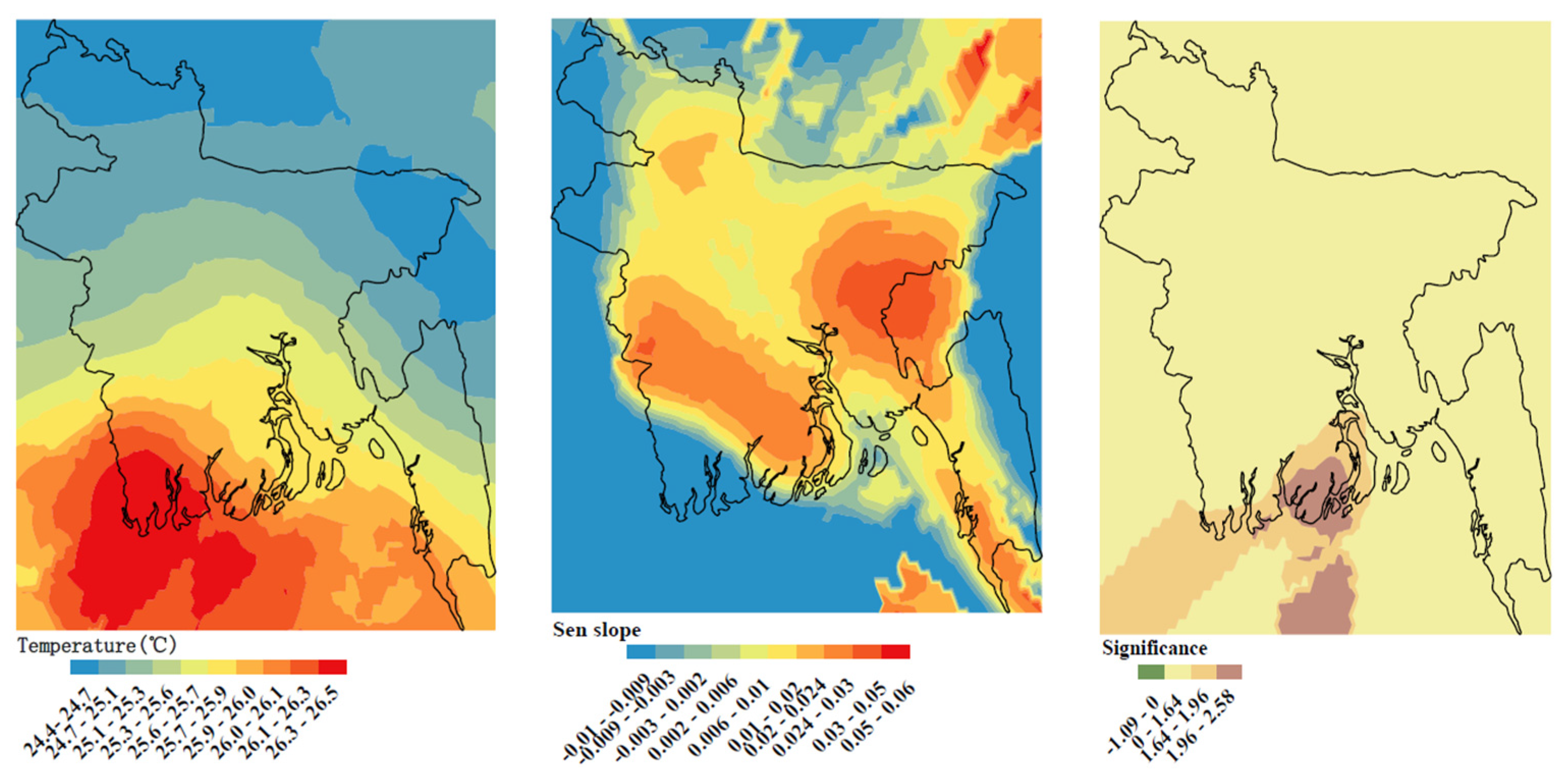
Finally, we used the high-resolution historical temperature data in Bangladesh during 1989–2018 as the input to the XGBoost-based forecast model to obtain high-resolution annual temperature forecast maps in Bangladesh during 2025–2035 (Figure 8). The annual average temperature in 2025–2035 gradually increases from north to south, reaching a maximum temperature of 26.5 °C in the southwest, which is almost consistent with average temperature distribution during 1989–2018 (Figure 8-left). Overall, the annual mean temperature is forecast to increase during 2025–2035, with at most 0.06 °C/year by Sen’s slope test (Figure 8-middle). However, the increasing trends were not significant in most areas, except for the middle coastal regions (Figure 8-right).
We performed the analysis of empirical orthogonal functions (EOF) analysis on annual mean temperature during 2025–2035 (Table 3. The cumulative variance of the first three EOF modes reached 59% cumulatively, i.e., the first EOF mode explained 27%, the second EOF model explained 17%, and the third EOF model explained 15%, and all three EOF modes passed the North significance test.
The first EOF mode (Figure 9, left) mainly showed double-phase features, with roughly a negative phase occurring northeast and southwest regions, and a positive phase occurring in the northwest region, central region, and middle coastal region. The associated time coefficient showed a downward trend (Figure 10-left). The spatial distribution of the second EOF mode showed a significant multi-phase effect (Figure 9, middle), where three positive phase peaks appeared in the northwest, east, and south regions, and the main negative phase peak appeared in the southeast region (Figure 9, middle). The third EOF mode mainly showed the east–west reverse phase feature and the time coefficient associated with the second/third EOF mode showed an upward trend (Figure 10).
6. Conclusions
Climate change has a serious impact on the agricultural production and economic development of Bangladesh. The generation of high-resolution temperature maps is a must for any poor countries like Bangladesh since these maps can reveal the climate patterns in observation blank regions in poor countries, and then help relevant departments to formulate policies to mitigate and adapt to climate change in a timely manner and support economic and agricultural development. Based on observed temperature data and longitude/latitude/altitude data of 34 meteorological observation stations in Bangladesh from 1989 to 2018, we developed an efficient data-driven downscaling technique to generate high spatial-resolution temperature distribution maps in Bangladesh directly from daily temperatures observed at 34 meteorological stations with irregular distribution. The main advantages of our method are: the input data are sparsely distributed, not gridded; there is no need to use a large number of GCM outputs, resulting in a very low computational cost; it makes full use of nonlinear links between topographic factors and climate factors.
The known climate forecasts by CMIP6 models must depend on a huge amount of input parameters and high computing resources. Many developing countries have not enough observations, computing resources, and financial support to run CMIP6 models. Moreover, the resolution of the CMIP6 model is just 1–2 degrees. In this study, we explore the data-driven high-resolution climate forecast directly from limited climate observations and generate a high-resolution temperature forecast map in Bangladesh during 2025–2035. This data-driven forecast technique is just at the beginning, more work needs to be undertaken in the future.
Although our study only focused on Bangladesh, the proposed data-driven downscaling and forecast techniques can be applied to any developing country with only irregularly distributed climate and environmental observations. Moreover, our techniques can also be used to generate high-resolution evolution maps for other climate and environmental factors, e.g., humidity, PM2.5, and wind speed. In the future, we will explore these aspects.
Author Contributions
All authors are co-first authors. Conceptualization, Z.Z.; methodology, Z.Z.; software, Y.W. and J.Y.; formal analysis, Y.W., J.Y., Z.Z., L.C.D. and M.J.C.C.; investigation, L.C.D.; resources, L.C.D.; data curation, L.C.D.; writing—original draft preparation, Y.W., J.Y., Z.Z. and L.C.D.; writing—review and editing, Z.Z., L.C.D. and M.J.C.C. All authors have read and agreed to the published version of the manuscript.
Funding
The corresponding author was supported by the European Commission Horizon 2020 Framework Program No. 861584 and the Taishan Distinguished Professor Fund No. 20190910.
Institutional Review Board Statement
Not applicable.
Informed Consent Statement
Not applicable.
Data Availability Statement
Data available on request due to restrictions.
Conflicts of Interest
The authors declare no conflicts of interest.
References
- IPCC. Climate Change: The Physical Science Basis; Cambridge University Press: Cambridge, UK, 2021. [Google Scholar]
- Chou, C.; Lan, C.W. Changes in the Annual Range of Precipitation under Global Warming. J. Clim. 2012, 25, 222–235. [Google Scholar] [CrossRef]
- Shahid, S.; Behrawan, H. Drought risk assessment in the western part of Bangladesh. Nat. Hazards 2018, 46, 391–413. [Google Scholar] [CrossRef]
- Islam, M.N.; Van Amstel, A.; Islam, M.N.; Tamanna, S.; van Amstel, A.; Noman, M.; Ali, M.S.; Aparajita, D.M.; Roy, P.; Tanha, S.R.; et al. Climate change impact and comprehensive disaster management approach in Bangladesh: A review. In Bangladesh II: Climate Change Impacts, Mitigation and Adaptation in Developing Countries; Springer: Cham, Switzerland, 2021; Volume 2021, pp. 1–39. [Google Scholar]
- Hashmi, M.Z.; Shamseldin, A.Y.; Melville, B.W. Statistical downscaling of watershed precipitation using Gene Expression Programming (GEP). Environ. Model. Softw. 2011, 26, 1639–1646. [Google Scholar] [CrossRef]
- Yhang, Y.-B.; Sohn, S.-J.; Jung, I.-W. Application of dynamical and statistical downscaling to east Asian summer precipitation for finely resolved datasets. Adv. Meteorol. 2017, 2017, 2956373. [Google Scholar] [CrossRef]
- Zhang, Z. Environmental Data Analysis, 2nd ed.; DeGruyter: Berlin, Germany, 2023. [Google Scholar]
- Wilby, R.L.; Dawson, C.W.; Barro, E.M. SDSM—A decision support tool for the assessment of regional climate change impacts. Environ. Model. Softw. 2002, 17, 147–159. [Google Scholar] [CrossRef]
- Wilby, R.L.; Dawson, C.W. The statistical downscaling model: Insights from one decade of application. Int. J. Clim. 2013, 33, 1707–1719. [Google Scholar] [CrossRef]
- Shahriar, S.A.; Siddique, M.A.M.; Rahman, S.M.A. Climate change projection using statistical downscaling model over Chittagong Division, Bangladesh. Meteorol. Atmos. Phys. 2021, 133, 1409–1427. [Google Scholar] [CrossRef]
- Rana, M.M.; Adhikary, S.K. Climate change projection over southwest coastal region of Bangladesh using statistical downscaling model. AIP Conf. Proc. 2023, 2713, 050016. [Google Scholar]
- Huth, R.; Kliegrová, S.; Metelka, L. Non-linearity in statistical downscaling: Does I bring an improvement for daily temperature in Europe? Int. J. Clim. 2008, 28, 465–477. [Google Scholar] [CrossRef]
- Han, Y.; Yang, J.; Das, L.C. Evaluation of SDSM Models for climate predictions in Bangladesh. Int. J. Big Data Min. Glob. Warm. 2023, 5, 2350003. [Google Scholar] [CrossRef]
- Alamgir, M.; Ahmed, K.; Homsi, R.; Dewan, A.; Wang, J.-J.; Shahid, S. Downscaling and Projection of Spatiotemporal Changes in Temperature of Bangladesh. Earth Syst. Environ. 2019, 3, 381–398. [Google Scholar] [CrossRef]
- Hasan, M.A.; Islam, A.K.M.S.; Akanda, A.S. Climate projections and extremes in dynamically downscaled CMIP5 model outputs over the Bengal delta: A quartile based bias-correction approach with new gridded data. Clim. Dyn. 2018, 51, 2169–2190. [Google Scholar] [CrossRef]
- Hasan, M.K.; Kumar, L.; Gopalakrishnan, T. Inundation modelling for Bangladeshi coasts using downscaled and bias-corrected temperature. Clim. Risk Manag. 2020, 27, 100207. [Google Scholar] [CrossRef]
- Jing, W.; Yang, Y.; Yue, X.; Zhao, X. A Comparison of Different Regression Algorithms for Downscaling Monthly Satellite-Based Precipitation over North China. Remote Sens. 2016, 8, 835. [Google Scholar] [CrossRef]
- Montans, F.J.; Chinesta, F.; Gomez-Bombarelli Kutz, J.N. Data-driven modeling and learning in science and engineering. Comptes Rendus Mec. 2019, 347, 845–855. [Google Scholar] [CrossRef]
- Zhang, H.; Wu, P.; Yin, A.; Yang, X.; Zhang, M.; Gao, C. Prediction of soil organic carbon in an intensively managed reclamation zone of eastern China: A comparison of multiple linear regressions and the random forest model. Sci. Total Environ. 2017, 592, 704–713. [Google Scholar] [CrossRef] [PubMed]
- Li, S.B.; Paoli, R. Comparison of Machine Learning Models for Data-Driven Aircraft Icing Severity Evaluation. J. Aerosp. Inf. Syst. 2021, 18, 973–977. [Google Scholar] [CrossRef]
- Nguyen, K.A.; Seeboonruang, U.; Chen, W.L. Projected Climate Change Effects on Global Vegetation Growth: A Machine Learning Approach. Environments 2023, 10, 204. [Google Scholar] [CrossRef]
- Trinh, T.; Luu, B.T.; Le, T.H.T.; Nguyen, D.H.; Van Tran, T.; Van Nguyen, T.H.; Nguyen, K.Q.; Nguyen, L.T. A comparative analysis of weight-based machine learning methods for landslide susceptibility mapping in Ha Giang area. Big Earth Data 2023, 7, 1005–1034. [Google Scholar] [CrossRef]
- Eltazarov, S.; Bobojonov, I.; Kuhn, L.; Glauben, T. Improving risk reduction potential of weather index insurance by spatially downscaling gridded climate data—A machine learning approach. Big Earth Data 2023, 7, 937–960. [Google Scholar] [CrossRef]
- Zhang, D.; Qian, L.; Mao, B.; Huang, C.; Huang, B.; Si, Y. A Data-Driven Design for Fault Detection of Wind Turbines Using Random Forests and XGboost. IEEE Access 2018, 6, 21020–21031. [Google Scholar] [CrossRef]
- Li, S.; Qin, J.; He, M.; Paoli, R. Fast Evaluation of Aircraft Icing Severity Using Machine Learning Based on XGBoost. Aerospace 2020, 7, 36. [Google Scholar] [CrossRef]
- Rahman, M.M.; Rafiuddin, M.; Alam, M.M.; Kusunoki, S.; Kitoh, A.; Giorgi, F. Summer monsoon rainfall scenario over Bangladesh using a high-resolution AGCM. Nat. Hazards 2013, 69, 793–807. [Google Scholar] [CrossRef]
- Mallick, J.; Salam, R.; Islam, H.M.T.; Shahid, S.; Kamruzzaman, M.; Pal, S.C.; Bhat, S.A.; Elbeltagi, A.; Rodrigues, T.R.; Ibrahim, S.M.; et al. Recent changes in temperature extremes in subtropical climate region and the role of large-scale atmospheric oscillation patterns. Theor. Appl. Clim. 2022, 148, 329–347. [Google Scholar] [CrossRef]
- Shamshirband, S.; Hashemi, S.; Salimi, H.; Samadianfard, S.; Asadi, E.; Shadkani, S.; Kargar, K.; Mosavi, A.; Nabipour, N.; Chau, K.W. Predicting Standardized Streamflow index for hydrological drought using machine learning models. Eng. Appl. Comput. Fluid Mech. 2020, 14, 339–350. [Google Scholar] [CrossRef]
- Chagas, C.d.S.; de Carvalho Junior, W.; Bhering, S.B.; Calderano Filho, B. Spatial prediction of soil surface texture in a semiarid region using random forest and multiple linear regressions. Catena 2016, 139, 232–240. [Google Scholar] [CrossRef]
- Guo, P.T.; Li, M.F.; Luo, W.; Tang, Q.F.; Liu, Z.W.; Lin, Z.M. Digital mapping of soil organic matter for rubber plantation at regional scale: An application of random forest plus residuals kriging approach. Geoderma 2015, 237, 49–59. [Google Scholar] [CrossRef]
- Bagalkot, N.; Keprate, A.; Orderløkken, R. Combining Computational Fluid Dynamics and Gradient Boosting Regressor for Predicting Force Distribution on Horizontal Axis Wind Turbine. Vibration 2021, 4, 248–262. [Google Scholar] [CrossRef]
- Elnashar, A.; Zeng, H.; Wu, B.; Zhang, N.; Tian, F.; Zhang, M.; Zhu, W.; Yan, N.; Chen, Z.; Sun, Z.; et al. Downscaling TRMM Monthly Precipitation Using Google Earth Engine and Google Cloud Computing. Remote Sens. 2020, 12, 3860. [Google Scholar] [CrossRef]
- Xiong, X.; Guo, X.; Zeng, P.; Zou, R.; Wang, X. A short-term wind power forecast method via xgboost hyperparameters optimization. Front. Energy Res. 2022, 2022, 574. [Google Scholar]
- Yadav, S.; Shukla, S. Analysis of k-Fold Cross-Validation over Hold-Out Validation on Colossal Datasets for Quality Classification. In Proceedings of the 2016 IEEE 6th International Conference on Advanced Computing (IACC), Bhimavaram, India, 27–28 February 2016; pp. 78–83. [Google Scholar]
- Pedregosa, F.; Varoquaux, G.; Gramfort, A.; Michel, V.; Thirion, B.; Grisel, O.; Blondel, M.; Prettenhofer, P.; Weiss, R.; Dubourg, V.; et al. Scikit-Learn: Machine Learning in Python. J. Mach. Learn. Res. 2011, 12, 2825–2830. [Google Scholar]
- Wang, Y.; Sun, S.; Chen, X.; Zeng, X.; Kong, Y.; Chen, J.; Guo, Y.; Wang, T. Short-term load forecasting of industrial customers based on SVMD and XGBoost. Int. J. Electr. Power Energy Syst. 2021, 129, 106830. [Google Scholar] [CrossRef]
- Sun, B.; Sun, T.; Jiao, P. Spatio-Temporal Segmented Traffic Flow Prediction with ANPRS Data Based on Improved XGBoost. J. Adv. Transp. 2021, 1, 1–24. [Google Scholar] [CrossRef]
Figure 1.
The distribution of 34 meteorological stations in Bangladesh.

Figure 2.
Comparison between downscaled temperature by GBR, RF, SVM, and observed temperature.

Figure 3.
Taylor diagram of downscaled temperatures for different models.

Figure 4.
Spatial distribution of mean annual temperature map in Bangladesh by GBR, RF, and SVM.

Figure 5.
Effect of topographic factors on temperature in Bangladesh, from left to right: longitude, latitude, and altitude.
Figure 5.
Effect of topographic factors on temperature in Bangladesh, from left to right: longitude, latitude, and altitude.

Figure 6.
Spatial distribution of monthly mean temperature in Bangladesh during 1989–2018 (a–l).


Figure 7.
Comparison of predicted and observed monthly temperatures in Bangladesh.

Figure 8.
Spatio-temporal distribution (left), annual trends (middle), and significance (right) of annual temperature in Bangladesh during 2025–2035.
Figure 8.
Spatio-temporal distribution (left), annual trends (middle), and significance (right) of annual temperature in Bangladesh during 2025–2035.

Figure 9.
(From left to right) The first three EOF modes for annual temperature in Bangladesh during 2025–2035.
Figure 9.
(From left to right) The first three EOF modes for annual temperature in Bangladesh during 2025–2035.

Figure 10.
(From left to right) The time coefficient associated with the first three EOF modes.


Table 1.
Geographical locations of 34 meteorological stations (source: Bangladesh Meteorological Department).
Table 1.
Geographical locations of 34 meteorological stations (source: Bangladesh Meteorological Department).
| Station | Latitude | Longitude | Elevation | Zone | Station | Latitude | Longitude | Elevation | Zone |
|---|---|---|---|---|---|---|---|---|---|
| Dhaka | 23.7 | 90.4 | 8 | Plain | Feni | 23.0 | 91.4 | 6 | Plain |
| Sylhet | 24.9 | 91.8 | 34 | Mountain | Patuakhali | 23.4 | 90.3 | 2 | Plain |
| Mymensingh | 24.7 | 90.4 | 18 | Plain | chuadanga | 23.6 | 88.9 | 1 | Plain |
| Faridpur | 23.6 | 89.8 | 8 | Plain | Mungla | 22.6 | 89.5 | 4 | Plain |
| Khulna | 22.8 | 89.5 | 3 | Plain | Chandpur | 23.2 | 90.7 | 6 | Plain |
| Chittagong | 22.3 | 91.8 | 4 | Coastal | Sandwip | 22.5 | 91.4 | 2 | Coastal |
| Cox’s Bazar | 21.4 | 92 | 2 | Coastal | Bhola | 22.6 | 90.6 | 4 | Coastal |
| Jessore | 23.2 | 89.2 | 6 | Plain | Teknaf | 20.8 | 92.3 | 6 | Coastal |
| Satkhira | 22.7 | 89.1 | 4 | Plain | Sydpur | 24.9 | 88.9 | 25 | Mountain |
| Barisal | 22.7 | 90.4 | 3 | Plain | Srimangal | 24.3 | 91.7 | 22 | Mountain |
| Bogra | 24.8 | 89.4 | 18 | Mountain | Madaripur | 23.2 | 90.2 | 8 | Plain |
| Rangpur | 25.8 | 89.3 | 33 | Mountain | Kutubdia | 21.8 | 91.8 | 2 | Coastal |
| Dinajpur | 26.1 | 89.1 | 34 | Mountain | Rangamati | 22.5 | 92.2 | 63 | Mountain |
| Rajshahi | 24.3 | 88.7 | 17 | Mountain | MaijdeeCourt | 22.8 | 91.1 | 5 | Plain |
| Tangail | 24.3 | 89.9 | 1 | Plain | Hatiya | 22.5 | 90.2 | 6 | Coastal |
| Ishurdi | 24.1 | 89.1 | 13 | Plain | Sitakunda | 22.4 | 91.1 | 6 | Plain |
| Comilla | 23.4 | 91.2 | 9 | Plain | Khepupara | 21.9 | 90.2 | 2 | Coastal |
Table 2.
Validation results of downscaled temperature data.
| Models | |||
|---|---|---|---|
| MLR | 0.74 | 0.26 | 0.21 |
| SVM | 0.95 | 0.11 | 0.10 |
| RF | 0.96 | 0.10 | 0.10 |
| GBR | 0.98 | 0.06 | 0.08 |
Table 3.
EOF decomposition results of average temperature in Bangladesh from 2025 to 2035.
| Modes | Variance Contribution Rate | Cumulative Variance | North Salience |
|---|---|---|---|
| 1st | 27% | 25% | Significant |
| 2nd | 17% | 44% | Significant |
| 3rd | 15% | 59% | Significant |
Disclaimer/Publisher’s Note: The statements, opinions and data contained in all publications are solely those of the individual author(s) and contributor(s) and not of MDPI and/or the editor(s). MDPI and/or the editor(s) disclaim responsibility for any injury to people or property resulting from any ideas, methods, instructions or products referred to in the content. |
© 2024 by the authors. Licensee MDPI, Basel, Switzerland. This article is an open access article distributed under the terms and conditions of the Creative Commons Attribution (CC BY) license (https://creativecommons.org/licenses/by/4.0/).
Share and Cite
MDPI and ACS Style
Wu, Y.; Yang, J.; Zhang, Z.; Das, L.C.; Crabbe, M.J.C. High-Resolution Temperature Evolution Maps of Bangladesh via Data-Driven Learning. Atmosphere 2024, 15, 385. https://doi.org/10.3390/atmos15030385
AMA Style
Wu Y, Yang J, Zhang Z, Das LC, Crabbe MJC. High-Resolution Temperature Evolution Maps of Bangladesh via Data-Driven Learning. Atmosphere. 2024; 15(3):385. https://doi.org/10.3390/atmos15030385
Chicago/Turabian StyleWu, Yichen, Jiaxin Yang, Zhihua Zhang, Lipon Chandra Das, and M. James C. Crabbe. 2024. "High-Resolution Temperature Evolution Maps of Bangladesh via Data-Driven Learning" Atmosphere 15, no. 3: 385. https://doi.org/10.3390/atmos15030385
Note that from the first issue of 2016, this journal uses article numbers instead of page numbers. See further details here.