
Near-Future Projection of Sea Surface Winds in Northwest Pacific Ocean Based on a CMIP6 Multi-Model Ensemble


1
Marine Technology and Convergence Engineering, University of Science and Technology, Daejeon 34113, Republic of Korea
2
Coastal Disaster and Safety Research Department, Korea Institute of Ocean Science and Technology, Busan 49111, Republic of Korea
3
Research Center for Oceanography, National Research and Innovation Agency, Jakarta 14430, Indonesia
4
Ocean Climate Prediction Center, Korea Institute of Ocean Science and Technology, Busan 49111, Republic of Korea
5
Ocean Circulation and Climate Research Department, Korea Institute of Ocean Science and Technology, Busan 49111, Republic of Korea
*
Author to whom correspondence should be addressed.
Atmosphere 2024, 15(3), 386; https://doi.org/10.3390/atmos15030386
Submission received: 20 February 2024
/
Revised: 14 March 2024
/
Accepted: 20 March 2024
/
Published: 21 March 2024
(This article belongs to the Section Climatology)
Abstract
:Information about wind variations and future wind conditions is essential for a monsoon domain such as the Northwest Pacific (NWP) region. This study utilizes 10 Generalized Circulation Models (GCM) from CMIP6 to evaluate near-future wind changes in the NWP under various climate warming scenarios. Evaluation against the ERA5 reanalysis dataset for the historical period 1985–2014 reveals a relatively small error with an average of no more than 1 m/s, particularly in the East Asian Marginal Seas (EAMS). Future projections (2026–2050) indicate intensified winds, with a 5–8% increase in the summer season in the EAMS, such as the Yellow Sea, East Sea, and East China Sea, while slight decreases are observed in the winter period. Climate mode influences show that winter El Niño tends to decrease wind speeds in the southern study domain, while intensifying winds are observed in the northern part, particularly under SSP5-8.5. Conversely, summer El Niño induces higher positive anomalous wind speeds in the EAMS, observed in SSP2-4.5. These conditions are likely linked to El Niño-induced SST anomalies. For the application of CMIP6 surface winds, the findings are essential for further investigations focusing on the oceanic consequences of anticipated wind changes such as the ocean wave climate, which can be studied through model simulations.
1. Introduction
In recent decades, the Northwest Pacific (hereinafter NWP) ocean has been warming, manifested in extreme anomalous sea surface temperatures [1]. This warming has led to changes in atmospheric variables such as surface wind and has significant implications for regional ocean–atmosphere interactions [2]. Understanding projected wind changes is essential since it has a dominant role in ocean dynamics [3] and is crucial for marine safety. Additionally, information about future wind patterns is also important for ocean wave models [4,5]. For example, NWP is well known as a prominent spot for oceanic and atmospheric hazards such as typhoons or storm waves [6,7]. Thus, the quality of ocean wave forecasting system in this region depends on the quality of surface winds as one of the influential factors. The projected changes in sea surface winds also have broader significant implications for the occurrence and intensity of extreme events across the region. Stronger winds may escalate the severity of storms, consequently inducing extreme wave heights and leading to related hazards such as coastal flooding [8,9]. Changes in wind patterns can also influence regional climate dynamics, affecting precipitation and evaporation, which in turn can contribute to the onset or exacerbation of drought conditions [10,11]. So, insights into future changes in sea surface winds can provide a better understanding of the atmospheric processes driving extreme events in the NWP region.
Since the NWP is in a monsoon domain, the wind patterns in the NWP are mostly dominated by the East Asian Monsoon (EAM) [12]. The main features of the EAM occur in winter and summer, namely the East Asian Winter Monsoon (EAWM), which is driven by the differential heating between the Eurasia continent and the surrounding oceans [13], and the East Asian Summer Monsoon (EASM), which is generated by the increased heat source of the Tibetan Plateau [14]. Annual variations in the EAM produce strong southerlies in the EASM, bringing water vapor and precipitation to East Asia [15], and strong northerlies in the EAWM, which are commonly associated with severe snowstorms [16]. In accordance with annual warming, the EAM has also been affected by both natural and anthropogenic forcing [11], which are responsible for future changes [17].
Currently, the best tool to investigate future conditions of oceanic and atmospheric processes is the latest version of Coupled Model Intercomparison Project Phase 6 (CMIP6) [18] since it provides projections based on different Shared Socio-Economic Pathways (SSPs) and distinct radiative forcing scenarios. Previous studies have assessed the results of CMIP6 models in the NWP region, such as [19,20]. The authors mostly focused on the performance models, which suggested that CMIP6 models generally have sufficiently good skills to reproduce the annual trends and variability of atmospheric or oceanic variables such as surface winds and ocean temperatures. However, it is important to note that the composition of the chosen models may lead to varying statistical performance results of multi-model ensembles. Additionally, seasonal wind variations in the NWP can be influenced by remote climate variability, such as El Niño–Southern Oscillation (ENSO) [21]. For example, a study has indicated that El Niño events can alter atmospheric circulation in the NWP, leading to anomalous anticyclones during the summer season [22]. Despite these interactions, the expected changes in future wind patterns resulting from global warming effects and the influence of remote climate variability remain poorly investigated in this region.
Therefore, this study aims to (1) evaluate projected wind changes in the NWP using CMIP6 models for the near-future period of the mid-twenty-first century and (2) investigate wind changes based on climate variability, with a particular focus on El Niño. To attain these objectives, this paper is divided into several sections as follows: The datasets and methods used in this study are briefly introduced in Section 2. Section 3 provides a statistical evaluation of the CMIP6 models’ performance skills and highlights future wind changes under different global warming scenarios and under the influence of El Niño events. Section 4 contains a discussion about the possible mechanism behind the future wind changes. Lastly, the conclusions are presented in Section 5.
2. Materials and Methods
2.1. Datasets
The surface wind fields of ten General Circulation Models (GCMs) were employed from CMIP6 (see Table 1), covering historical (1985–2014) and near-future (2026–2050) periods. The selection of these models was based on their capacity to provide future projection data. The choice was also influenced by the requirement for the highest temporal resolution feasible, considering the intended application for input into wave model simulations. All CMIP6 models were freely available at https://esgf-node.llnl.gov/search/cmip6/, accessed on 31 December 2023, and detailed information about the data can be accessed from the Program for Climate Model Diagnosis and Intercomparison (PMCDI) through https://pcmdi.llnl.gov/CMIP6/ (accessed on 31 December 2023). Each GCM in CMIP6 has specific ensemble numbers which are determined by a variant label and indicated with the indices (r), (i), (p), and (f). These labels define ensemble number, initial method, perturbed physics, and forcing index, respectively. In this study, the initial ensemble (r1i1p1f1) of all models was used to avoid bias evaluation. The SSP2-4.5 and SSP5-8.5, which represent mid and high radiative forcing scenarios, were used to investigate future projection changes. Similarly, the monthly sea surface temperature (SST) from the same CMIP6 datasets were used to calculate the Nino3.4 index and examine the oceanic conditions as an air–sea coupling response in the future.
Furthermore, the wind fields from the ERA5 reanalysis dataset, which has been developed by the European Centre for Medium-Range Weather Forecasts (ECMWF) to replace ERA-interim, with 0.25° spatial grid resolution were applied as the reference for the evaluation of historical CMIP6 models. ERA5 incorporates several data from various kinds of observations such as buoys, satellites, and radiosondes into the model to produce long-record data [23] using the assimilation method. Thus, it has been widely used in climate studies to assess the accuracy of model outputs [24,25].
2.2. Methods
Following previous studies [26,27], since the CMIP6 and ERA5 have different resolutions, bilinear interpolation was applied to regrid the available data into a uniform resolution. This study then used a 0.5° × 0.5° common grid for the comparison and convenience purposes. The historical CMIP6 wind fields were firstly evaluated quantitively by Taylor diagram. It provides a graphical summary of the main statistical components, such as correlation coefficient (R), standard deviation (STD), and root mean square difference (RMSD) [28]. A model skill assessment was also carried out by calculating several performance metrics such as Taylor Skill Score (SS) [29,30], Mielke Measure (M-Score) [31,32], Nash–Sutcliffe Efficiency (NSE) [33], and Index of Agreement (IA). The SS is expressed as the following equation:
where SDR is the standard deviation ratio between the CMIP6 models against ERA5, and represents the maximum of R (1 for this study). An excellent model performance is indicated when the SS score approaches 1. Furthermore, the M-Score was calculated as follows:
where the subscript x and y denote model (CMIP6) and reference (ERA5) field, respectively, V is defined as the variance, G is the domain-averaged of variable (wind), and MSE is the mean square error. The M-score ranges from 0 to 800, with 0 denoting a model with no skill.
Considering both the mean state and variability of the modeled and observed values, the NSE and IA was calculated using the following formulas:
where is the observed value at time , is the modeled value, is the mean of the observed data, and n indicates the total number of assessed variables. For NSE, the satisfactory models yield a score approaching 1, with higher values indicating better performance. On the other hand, a negative NSE signifies large bias models, while a score approaching 0 implies that the modeled results closely approximate the observed mean value. Like the NSE, the models are in good agreement with the reference when the IA’s score is close to 1.
Secondly, the Multi-Model Mean (MMM) over 10 models was also calculated using the common grid and used as the basis for historical comparison and future wind speed change analysis. This method is widely practiced in GCM future projection studies to alleviate individual model bias [18]. To determine the relative future changes (RC), the MMM absolute change was divided by its climatology as shown in the following expression. A substantial positive RC values suggest a future enhancement in wind speed. In this study, the seasonal analysis is defined as the boreal summer (June–August, JJA) and winter (December–February: DJF).
Furthermore, ENSO events in this study were identified using the Nino3.4 index, which was calculated from the SST anomalies in the Nino3.4 region (5° S–5° N, 120°–170° W). The historical period was marked as the baseline. It is worth noting that this study is focused on El Niño only since the NWP SST exhibits more response following El Nino [34].
Considering the warming effect of the model scenarios, the El Niño episodes were selected when the detrended (rather than the original) index [35] exceeded the threshold of 0.5 °C. Subsequently, an examination of future seasonal wind changes under El Niño conditions was conducted using composite analysis.
3. Results
3.1. Perfomance of CMIP6 Models in Historical Period (1985–2014)
The performance evaluation of wind speed from the CMIP6 models is presented in Figure 1. In general, all models are in good agreement with ERA5, with the correlation being more than 0.8, except for BCC-CSM2-MR. The other statistics show a range of 0.469–0.519 m/s for RMSE and 0.781 to 1.09 m/s for STD. As expected, the MMM could improve the model performance, as indicated by the higher correlation (0.918) and lower RMSD (0.384 m/s) compared to individual models. Although the STD value of MMM (0.968 m/s) is not as close to ERA5 (0.861 m/s) as that of BCC-CSM2-MR (0.857 m/s), it still reflects a substantial enhancement over the individual model performance. The robust correlations between models and ERA5 suggest that the CMIP6 models generally capture observed wind speed patterns effectively.
The summary of the quantitative assessment provides a clearer insight into the performance of CMIP6. While the overall performance appears to be commendable, as indicated in Table 2, there is a notable variation in the NSE metric among the models. However, this assessment further validates the exceptional performance of the MMM, consistently ranking first across all metrics. Furthermore, in terms of individual skill, IPSL-CM6A-LR and MIROC6 perform best in the total rank, closely followed by ACCESS-CM2.
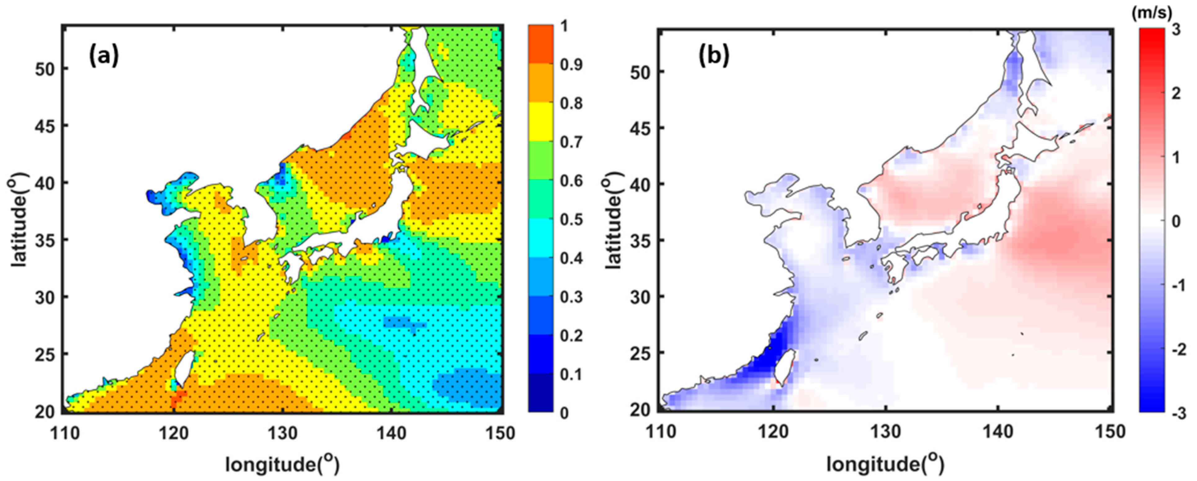
To better understand the CMIP6 skill over the study area, Figure 2 presents the spatial MMM correlation and bias error (deviation between ERA5 and MMM). The spatial pattern consistently reveals a significant positive correlation (p < 0.05) across the domain (Figure 2a), with the higher values mostly being found in the East Asian Marginal Seas (EAMS), particularly in the center of East Sea (ES), ranging from 0.8 to 0.9. Meanwhile, a moderate relationship is observed in the Yellow Sea (YS) and the East China Sea (ECS). On the other hand, the bias error (Figure 2b) indicates variations across the region, highlighting a prevalent underestimation of 0.34 m/s and 1.02 m/s in the YS and ECS, respectively. An overestimation is observed in the ES with an average of less than 0.2 m/s.
Additionally, the spatial map depicting wind fields (magnitude and direction) for the annual and seasonal mean are shown in Figure 3. Overall, the observed patterns exhibit a similarity between MMM wind direction and ERA5 in both annual and seasonal mean. Meanwhile, it consistently reveals biases in the magnitude (Figure 3a,b). In particular, the winter season (Figure 3c,d) exhibits overestimations in the northern domain, especially in the ES, where MMM magnitudes can reach up to 8 m/s compared to ERA5 values of approximately 7 m/s. Conversely, underestimations in the southern domain, covering YS and ECS, are observed during the summer season, with ERA5 magnitudes ranging from 2.5 to 4 m/s and MMM values ranging from 1.5 to 3 m/s (Figure 3e,f). These conditions display the MMM’s ability in reproducing seasonal surface wind patterns of ERA5 in the region, albeit facing challenges, inaccurately representing conditions in the ES (YS and ECS) during winter (summer).
3.2. CMIP6 MMM Wind Future Projection
To determine the temporal changes, the time series of MMM wind speed based on domain-averaged is as depicted in Figure 4. During the historical period, the trend of annual wind speed exhibits a slight decline at a rate of −0.020 m/s per decade (Figure 4a), indicating the weakened winds in a 30-year period. This historical declining trend is suggested to be influenced by winter winds, as indicated by the same decreasing trend at −0.003 m/s per decade (Figure 4b). In contrast, the summer mean wind speed shows an increasing trend at 0.004 m/s per decade (Figure 4c). The MMM future changes are also evaluated in the 2015–2050 period. A contrast trend variation is observed in SSP2-4.5, where the positive (negative) trend occurs at a rate of 0.003 m/s per decade and 0.006 per decade (−0.001 m/s per decade) for annual and winter (summer) mean values, respectively. Meanwhile, SSP5-8.5 forecasts a reduction in wind speed for all cases—at −0.002 m/s per decade for the annual mean and −0.003 m/s per decade (−0.001 m/s per decade) for the winter (summer) mean. The different trends in the future projections underscore the sensitivity of wind patterns to the different emission scenarios, highlighting the role that human activities play in shaping future climatic conditions.
Furthermore, the spatial changes of projected winds during the near-future period under two SSP scenarios are presented in Figure 5. The percentage of change based on Equation (5) is calculated with respect to the historical period of annual and seasonal mean values (refer to Figure 3b,d,f). In general, the future winds blow in similar directions to those in the historical period. Spatial-averaged results reveal relatively minor differences, typically around 4–5° counter-clockwise from the historical, particularly in the annual and summer mean. Notably, higher-emission scenarios exhibit slightly larger disparities in these periods. However, winter wind patterns remain remarkably stable, with variations of less than 1° across both scenarios (Table 3). These findings imply that the wind direction will change more in the summer. For clarity, black vector arrows have been placed on the graph.
Meanwhile, significant variations in wind magnitudes are observed across the region. Future change patterns indicate similarities between the annual and winter mean (Figure 5a–d), with the southern (northern) part of the NWP likely experiencing weakened (intensified) winds. Notably, while the southern region within the boundaries of 130–150° E and 20–30° N also shows a decline in wind speed, the EAMS region is projected to experience the most pronounced intensification in future summers (Figure 5e,f). These changes suggest a robust warming trend in summer wind speeds in the future.
Upon closer examination, spatial maps also underscore the regional variability of EAMS in response to emission scenarios. In the annual mean, although there are relatively insignificant positive changes in both SSPs, a more pronounced decrease of up to 8% is observed in SSP5-8.5 offshore of ECS, compared to the lower scenarios. The conditions in both SSPs are not markedly different during the winter period, but the decrease in winds of around 5% is more widespread across the YS and ECS. Furthermore, substantial increases in winds are observed in summer for both scenarios, ranging from 5% to 8% in EAMS.
3.3. Wind Changes under El Niño Conditions
In the context of climate mode influence, the future wind changes under El Niño events in summer and winter are presented in Figure 6. During the future winter El Niño, the EAMS region is mostly covered by anomalous negative wind speed, under the lower radiative scenario (SSP2-4.5) (Figure 6a). As shown in the figure, it is suggested that the strong anomalous southeasterlies reduce the climatological wind speed due to the contrast direction. On the other hand, the increasing wind speed is more pronounced and more spread in the northern domain, covering mostly the ES under SSP5-8.5. However, the ECS consistently exhibits a negative anomaly, while the YS experiences a slight increase compared to the lower scenario (Figure 6b).
Conversely, during the summer El Niño events, a reversal of the observed pattern is evident. Specifically, under the influence of SSP2-4.5, the EAMS is predominantly characterized by positive wind speed anomalies. Remarkably, the ES maintains a positive anomaly, indicating intensified wind speed in the future (Figure 6c). On the other hand, when considering SSP5-8.5, the increased wind speeds in the EAMS, such as the ES and YS, are not as pronounced as those under SSP2-4.5. Meanwhile, the decreased wind speeds appear in part of the ECS (Figure 6d).
4. Discussion
The findings presented in this study show a comprehensive evaluation of the CMIP6 models’ performance in simulating wind speed over the historical period (1985–2014) and provide insights into future projections as well as the influence of El Niño in the near-future period (2026–2050). In the historical period, the CMIP6 models generally demonstrate good agreement with ERA5, with a robust correlation above 0.8 for most models. The Multi-Model Mean (MMM) emerges as a powerful tool, exhibiting significant model performance, with higher correlations and lower RMSD compared to the individual model (Figure 1). The results show that MMM could reduce the individual model biases, as also shown in other studies [36,37,38]. Notably, IPSL-CM6A-LR, MIROC6, and ACCES-CM2 exhibit outstanding individual skill, reinforcing the utility of MMM. Furthermore, in a previous study [20], the authors ranked ACCES-CM2 as the best for the wind variable in the NWP based on a performance score using the normalized RMSD and Taylor skill score. Therefore, the findings of this study also provide information about the alternative best choices aside from ACCES-CM2 in terms of individual CMIP6 model usage, as the earlier study did not include considerations for IPSL-CM6A-LR and MIROC6.
Spatial analysis reveals a positive correlation between MMM and ERA5 across the study area, particularly in the EAMS. However, local biases may arise due to potential extreme events, such as strong northerly winds during the winter period [39], which can lead to severe snowstorms [15] and extreme waves in the ES [6,40], as well as extreme wind speeds associated with the typhoon activities [41,42] in the southern domain (ECS) during the summer season. Despite these challenges, the findings emphasize MMM’s ability to reproduce the seasonal variations of ERA5, as shown in Figure 3.
Examining temporal changes, the historical period shows a slight decline in annual wind speed, possibly driven by decreased winter winds, while summer winds exhibit an increasing trend (Figure 4), as also shown in Taiwanese waters [43]. More specifically, the wind speeds during the transitional period (2014–2015) between historical and future simulations exhibit a realistic transition regarding interannual variability patterns. In particular, the transition in the winter mean appears smoother, compared to the others, as the wind speeds in 2015 are not significantly different from those in 2014. For the annual mean, SSP5-8.5 predicts a higher value than SSP2-4.5, which is likely attributed to warming scenarios. This aligns with the observed upward phase in the historical years of 2013 and 2014. For the summer mean, all scenarios indicate higher values in 2015 than in 2014. Similar increases were also observed in historical periods such as the summer of 2002–2003 and 2006–2007. Thus, this suggests a reasonable transition between historical and future scenarios.
Future projections under different emission scenarios highlight the sensitivity of wind pattern. Spatially, the projected changes in wind magnitudes vary across the region, emphasizing regional variability in response to the emission scenarios. The results suggest a warming trend in summer wind speed, with notable differences in the magnitude of change compared to the annual and winter mean values (Figure 5). Utilizing projections derived from CMIP6 models provides a robust foundation for understanding climate dynamics, despite inherent limitations. While this study assessed 10 models from CMIP6, each contributes unique perspectives. Recognizing the diversity of models available in CMIP6, it is crucial to acknowledge that outputs from additional simulations may yield further insights and complement the findings presented here, enriching our understanding of future climate scenarios.
This study also investigates the impact of El Niño events on future wind changes. During winter El Niño, the EAMS region is mostly covered by negative anomalous wind speeds under SSP2-4.5, while intensified wind speeds are pronounced in the ES under SSP5-8.5. In contrast, a summer El Niño event results in high (low) positive wind anomalies in EAMS under SSP2-4.5 (5.85) (Figure 6). Even though the frequency of future El Niño events may not show significant changes (not shown), their amplitude may vary, resulting in different impacts on the atmospheric circulation, as illustrated in Figure 6. To determine the possible driver behind these conditions, we used spatial maps of global sea surface temperature (SST) under El Niño conditions in winter and summer, as presented in Figure 7. In general, the MMM of CMIP6 models could capture the El Niño-like pattern in both seasons and scenarios.
During the future winter El Niño, the warmer SST appear in northern part of the ES region under SSP2-4.5 (Figure 7a), compared to the SSP5-8.5 (Figure 7c). Consequently, the warmer SSTs are associated with the weakened wind speed, as shown in Figure 6a. This condition suggests that future warming could influence the winter wind speed changes. While [44] found that the most CMIP6 models have a weak performance for the air–sea coupling in the tropical pacific, this result also suggests that MMM air–sea coupling is sufficient in the ES region.
Meanwhile, the increasing wind speeds in the EAMS during the summer El Niño (Figure 6b) coexist with the high positive anomalous SST during SSP2-4.5 (Figure 7b). A similar pattern is also observed in SSP5-8.5, where the less pronounced wind speeds in the EAMS (Figure 6d) are associated with the cooler SST (Figure 7d). Reference [45] argued that the increasing SST could enhance the maximum potential of typhoons. With the warm SST, moist air rises from the ocean surface, it cools and condenses, creating low pressure at the surface, which causes the wind to circulate it and causes the typhoon’s growth. The findings suggest that the stronger wind in the future summer El Niño under SSP2-4.5 could be associated with the appearance of typhoon activities. Additionally, the observed contrasting patterns of equatorial warming between SSP2-4.5 and SSP5-8.5 in the summer versus the winter (Figure 7) could be attributed to varying levels of greenhouse gases and associated climate scenarios. This condition also raises the possibility that any substantial bias in SST during the historical period related to ENSO, as noted in [46], may influence the future projections of ENSO. This highlights the importance of further investigation to fully understand the complexities of future climate dynamics.
5. Conclusions
In conclusion, most of the CMIP6 models in this study demonstrated good agreement with the reference (ERA5), exhibiting a correlation exceeding 0.8, except for BCC-CSM2-MR. The results indicated that the MMM method effectively mitigates the individual biases, showcasing improved performance in reproducing observed wind patterns. Seasonal variations show MMM’s ability to capture the ERA5 pattern, although it faced challenges, inaccurately representing conditions in several parts of NWP such as the ES (YS-ECS) during winter (summer). Spatially, the future changes highlight the regional variability within EAMS in response to different emission scenarios. It suggests that the future wind changes ranging from 5% to 8% in EAMS are a consequence of warming scenarios in summer wind speed. The investigation of future wind changes under El Niño events shows that the El Niño-induced wind anomalies could directly impact the winter wind speeds through the wind–SST relationship with the warmer SST in the ES under SSP2-4.5. On the other hand, the stronger EAMS winds correspond to the higher SST under SSP2-4.5 compared to SSP5-8.5, suggesting that there is a possibility of the typhoon activities’ influence during the future summer El Niño. The findings highlight the complex interplay between natural variability and anthropogenic forcing, represented by SSPs, providing a foundation for enhancing our understanding of future climate scenarios in the region of study. The results contribute to the broader discourse on climate change’s impacts on regional atmospheric dynamics.
Future works should focus on the consequences of anticipated wind changes on oceans, such as ocean waves and their extreme conditions, due to their implications for adapting to and mitigating the impact of future extreme events.
Author Contributions
Conceptualization, A.B.; data curation, A.B.; visualization, A.B.; writing—original draft, A.B.; supervision, J.Y.; project administration, J.Y.; writing—review and editing, J.Y., C.J.J., M.K. and H.-W.K. All authors have read and agreed to the published version of the manuscript.
Funding
This research was supported by KIOST (PO0147A and PEA0231) and the Korea Institute of Marine Science & Technology Promotion (KIMST) funded by the Ministry of Oceans and Fisheries (20220431, Development of Simulation Technology for Maritime Spatial Policy).
Institutional Review Board Statement
Not applicable.
Informed Consent Statement
Not applicable.
Data Availability Statement
The data used in this study are freely available and can be downloaded through the mentioned link in the methodology section.
Acknowledgments
The authors thank the editors and anonymous reviewers for insightful comments to improve the manuscript. The first author thanks the UST Young Scientist+ Research Program 2022.
Conflicts of Interest
The authors declare no conflicts of interest.
References
- Hayashi, M.; Shiogama, H.; Emori, S.; Ogura, T.; Hirota, N. The Northwestern Pacific warming record in August 2020 occurred under anthropogenic forcing. Geophys. Res. Lett. 2021, 48, e2020GL090956. [Google Scholar] [CrossRef]
- Li, D.; Chen, Y.; Qi, J.; Zhu, Y.; Lu, C.; Yin, B. Attribution of the July 2021 record-breaking Northwest Pacific marine heatwave to global warming, atmospheric circulation, and ENSO. Bull. Am. Meteorol. Soc. 2023, 104, E291–E297. [Google Scholar] [CrossRef]
- Lohman, K.; Putrasahan, D.; von Storch, J.-S.; Gutjahr, O.; Jungclaus, J.H.; Haak, H. Response of northern north Atlantic and Atlantic meridional overturning circulation to reduced and enhanced wind stress forcing. J. Geophys. Res. Oceans 2021, 126, JC017902. [Google Scholar] [CrossRef]
- Lim, D.-U.; Suh, K.-D.; Mori, N. Regional projection of future extreme wave heights around Korean peninsula. Ocean. Sci. J. 2013, 48, 439–453. [Google Scholar] [CrossRef]
- Semedo, A.; Weisse, R.; Behrens, A.; Sterl, A.; Bengstsson, L.; Gunther, H. Projection of global wave climate change toward the end of twenty-first century. J. Clim. 2013, 26, 8269–8288. [Google Scholar] [CrossRef]
- Heo, K.-Y.; Choi, J.-Y.; Jeong, S.-H.; Kwon, J.-I. Characteristics of high swell-like waves on east coast of Korea observed by direct measurements and reanalysis data sets. J. Coast. Res. 2020, 95, 1433–1437. [Google Scholar] [CrossRef]
- Oh, S.M.; Moon, I.-J. Typhoon and storm surge intensity changes in a warming climate around the Korean Peninsula. Nat. Hazards 2013, 66, 1405–1429. [Google Scholar] [CrossRef]
- Cardone, V.J.; Callahan, H.; Chen, H.; Cox, A.T.; Morrone, M.A.; Swail, V.R. Global distribution and risk to shipping of very extreme sea states (VESS). Int. J. Climatol. 2015, 35, 69–84. [Google Scholar] [CrossRef]
- Son, D.; Jun, K.; Kwon, J.-I.; Yoo, J.; Park, S.-H. Improvement of wave predictions in in marginal seas around Korea through correction of simulated sea winds. Appl. Ocean Res. 2023, 130, 103433. [Google Scholar] [CrossRef]
- Qi, H.; Shan, X.; Chen, D.; Zhu, C.; Zhu, Y. Droughts near the northern fringe of the East Asian Summer Monsoon in China during 1470–2003. Clim. Chang. 2012, 110, 373–383. [Google Scholar]
- Chen, W.; Wang, L.; Feng, J.; Wen, Z.; Ma, T.; Yang, X.; Wang, C. Recent progress in studies of the variabilities and mechanisms of the East Asian Monsoon in a Changing Climate. Adv. Atmos. Sci. 2019, 36, 887–901. [Google Scholar] [CrossRef]
- Ha, K.-J.; Heo, K.-Y.; Lee, S.-S.; Yun, K.-S.; Jhun, J.-G. Variability in the East Asian monsoons: A review. Meteorol. Appl. 2012, 19, 200–215. [Google Scholar] [CrossRef]
- Ren, H.-L.; Huang, Y.; Chadwick, R.; Deng, Y. Decomposing East-Asian winter temperature and monsoonal circulation changes using timeslice experiments. Clim. Dyn. 2020, 54, 2297–2315. [Google Scholar] [CrossRef]
- Huang, R.H.; Zhou, L.T.; Chen, W. The progresses of recent studies on the variabilities of the East Asian monsoon and their causes. Adv. Atmos. Sci. 2003, 20, 55–69. [Google Scholar] [CrossRef]
- Chen, W.; Wang, L.; Xue, Y.K.; Sun, S.F. Variabilities of the spring river runoff system in East China and their relations to precipitation and sea surface temperature. Int. J. Climatol. 2009, 29, 1381–1394. [Google Scholar] [CrossRef]
- Chang, C.P.; Wang, Z.; Hendon, H. The Asian winter monsoon. In The Asian Monsoon; Wang, B., Ed.; Springer: Berlin/Heidelberg, Germany, 2006; pp. 89–127. [Google Scholar]
- Wu, Q.-Y.; Li, Q.-Q.; Ding, Y.-H.; Shen, X.-Y.; Zhao, M.-C.; Zhu, Y.-X. Asian summer monsoon responses to the change of land-sea thermodynamic contrast in a warming climate: CMIP6 projections. Adv. Clim. Chang. Res. 2022, 13, 205–217. [Google Scholar] [CrossRef]
- IPCC. Climate Change 2021: The Physical Science Basis; Contribution of Working Group I to the Sixth Assessment Report of the Intergovernmental Panel on Climate Change; Cambridge University Press: Cambridge, UK; New York, NY, USA, 2021. [Google Scholar]
- Badriana, M.R.; Lee, H.S. Statistical evaluation of monthly marine surface winds of CMIP6 GCMs in the western north Pacific. J. Jpn. Soc. Civ. Eng. 2019, 75, 1219–1224. [Google Scholar] [CrossRef]
- Oh, S.-G.; Kim, B.-G.; Cho, Y.-K.; Son, S.-W. Quantification of the performance of CMIP6 models for dynamic downscaling in the north Pacific and northwest Pacific oceans. Asia Pac. J. Atmos. Sci. 2023, 59, 367–383. [Google Scholar] [CrossRef]
- Wang, B.; Wu, R.G.; Fu, X.H. Pacific-East Asian teleconnection: How does ENSO affect east Asian climate? J. Clim. 2000, 13, 1517–1536. [Google Scholar] [CrossRef]
- Lee, S.-H.; Seo, K.-H.; Kwon, M. Combined effects of El Niño and the Pacific Decadal Oscillation on summertime circulation over East Asia. Asia Pac. J. Atmos. Sci. 2019, 55, 91–99. [Google Scholar] [CrossRef]
- Hersbach, H.; Bell, B.; Berrisford, P.; Hirahara, S.; Horányi, A.; Muñoz-Sabater, J.; Nicolas, J.; Peubey, C.; Radu, R.; Schepers, D.; et al. The ERA5 global reanalysis. Q. J. R. Meteorol. Soc. 2020, 146, 1999–2049. [Google Scholar] [CrossRef]
- Ali, Z.; Hamed, M.M.; Muhammad, M.K.I.; Iqbal, Z.; Shahid, S. Performance evaluation of CMIP6 GCMs for the projections of precipitation extremes in Pakistan. Clim. Dyn. 2023, 61, 4717–4732. [Google Scholar] [CrossRef]
- Usta, D.F.D.; Parra, R.R.T. Projected wind changes in the Caribbean Sea based on CMIP6 models. Clim. Dyn. 2023, 60, 3713–3727. [Google Scholar] [CrossRef]
- Chen, C.-A.; Hsu, H.-H.; Liang, H.-C. Evaluation and comparison of CMIP6 and CMIP5 model performance in simulating the seasonal extreme precipitation in the western north Pacific and east Asia. Weather Clim. Extrem. 2021, 31, 100303. [Google Scholar] [CrossRef]
- Kim, K.-H.; Shim, P.-S.; Shin, S. An alternative bilinear interpolation method between spherical grids. Atmosphere 2019, 10, 123. [Google Scholar] [CrossRef]
- Taylor, K.E. Summarizing multiple aspects of model performance in a single diagram. J. Geophys. Res. Atmos. 2001, 106, 7183–7192. [Google Scholar] [CrossRef]
- Ito, R.; Shiogama, H.; Nakaegawa, T.; Takayabu, I. Uncertainties in climate change projection covered by the ISIMIP and CORDEX model subsets from CMIP5. Geosci. Model Dev. 2020, 13, 859–872. [Google Scholar] [CrossRef]
- Krishnan, A.; Bhaskaran, P.K.; Kumar, P. CMIP5 model performance of significant wave heights over the Indian Ocean using COWCLIP datasets. Theor. Appl. Climatol. 2021, 145, 377–392. [Google Scholar] [CrossRef]
- Hemer, M.A.; Trenham, C.E. Evaluation of a CMIP5 derived dynamical global wind wave climate model ensemble. Ocean Model. 2016, 103, 190–203. [Google Scholar] [CrossRef]
- Watterson, I.G. Improved simulation of regional climate by global models with higher simulation: Skill scores correlated with grid length. J. Clim. 2015, 28, 5985–6000. [Google Scholar] [CrossRef]
- Gou, J.; Miao, C.; Duan, Q.; Tang, Q.; Di, Z.; Liao, W.; Wu, J.; Zhou, R. Sensitivity analysis-based automatic parameter calibration of the VIC model for streamflow simulations over China. Water Resour. Res. 2020, 56, e2019WR025968. [Google Scholar] [CrossRef]
- Hardiman, S.C.; Dunstone, N.J.; Scaife, A.A.; Bett, P.E.; Li, C.; Lu, B.; Ren, H.-L.; Smith, D.M.; Stephan, C.C. The asymmetric response of Yangtze river basin summer rainfall to El Niño. Environ. Res. Lett. 2018, 13, 024015. [Google Scholar] [CrossRef]
- Kumar, P.; Min, S.-K.; Weller, E.; Lee, H.; Wang, X.L. Influence of climate variability on extreme ocean surface wave heights assessed from ERA-interim and ERA-20C. J. Clim. 2016, 29, 4031–4046. [Google Scholar] [CrossRef]
- Lei, X.; Xu, C.; Liu, F.; Song, L.; Cao, L.; Suo, N. Evaluation of CMIP6 models and multimodel ensemble for extreme precipitation over arid Central Asia. Remote Sens. 2023, 15, 2736. [Google Scholar] [CrossRef]
- Wu, J.; Shi, Y.; Xu, Y. Evaluation and projection of surface wind speed over China based on CMIP6 GCMs. J. Geophys. Res. Atmos. 2020, 125, e2020JD033611. [Google Scholar] [CrossRef]
- Zhao, L.; Jin, S.; Liu, X.; Wang, B.; Song, Z.; Hu, J.; Guo, Y. Assessment of CMIP6 model performance for wind speed in China. Front. Clim. 2021, 3, 735988. [Google Scholar] [CrossRef]
- Huang, R.H.; Chen, J.L.; Wang, L.; Lin, Z.D. Characteristics, processes and causes of the spatio-temporal variabilities of the East Asian monsoon system. Adv. Atmos. Sci. 2012, 29, 910–942. [Google Scholar] [CrossRef]
- Lee, H.S.; Komaguchi, T.; Yamamoto, A.; Hara, M. Wintertime extreme storm waves in the East Sea: Estimation of extreme storm waves and wave-structure interaction study in the Fushiki Port, Toyama Bay. J. Korean Soc. Coast. Ocean Eng. 2013, 25, 335–347. [Google Scholar] [CrossRef]
- Ling, S.; Lu, R. Tropical cyclones over the western north Pacific strengthen the East Asia-Pacific pattern during summer. Adv. Atmos. Sci. 2022, 39, 249–259. [Google Scholar] [CrossRef]
- Wang, B.; Zhang, Q. Pacific-East Asian teleconnection. Part II: How the Philippine Sea anomalous anticyclone is established during El Niño development. J. Clim. 2002, 15, 3252–3265. [Google Scholar] [CrossRef]
- Chien, H.; Cheng, H.-Y.; Chiou, M.-D. Wave climate variability of Taiwan waters. J. Oceanogr. 2014, 70, 133–152. [Google Scholar] [CrossRef]
- Wang, M.; Yuan, C.; Liu, J.; Wei, Y.; Wu, J.; Luo, J. Underestimated relationship between westerly wind bursts and ENSO in CMIP6 models. Atmos. Ocean. Sci. Lett. 2023, 16, 100336. [Google Scholar] [CrossRef]
- Emmanuel, K.A. Increasing destructiveness of tropical cyclones over the past 30 years. Nature 2005, 436, 686–688. [Google Scholar] [CrossRef] [PubMed]
- Song, Z.; Liu, H.; Chen, X. Eastern equatorial Pacific SST seasonal cycle in global climate models: From CMIP5 to CMIP6. Acta Oceanol. Sin. 2020, 39, 50–60. [Google Scholar] [CrossRef]
Figure 1.
Taylor diagrams of monthly wind speed in the study area, displaying the statistical performance of the CMIP6 models and MMM with respect to ERA5 over the historical period (1985–2014).
Figure 1.
Taylor diagrams of monthly wind speed in the study area, displaying the statistical performance of the CMIP6 models and MMM with respect to ERA5 over the historical period (1985–2014).

Figure 2.
Spatial pattern of wind speed correlation (a) and bias error (b) in NWP ocean. The black dots in (a) indicate grid points with the confidence level >95%. The positive (negative) values in (b) denote overestimation (underestimation).
Figure 2.
Spatial pattern of wind speed correlation (a) and bias error (b) in NWP ocean. The black dots in (a) indicate grid points with the confidence level >95%. The positive (negative) values in (b) denote overestimation (underestimation).

Figure 3.
Spatial pattern of wind speed annual (a,b), winter (c,d) and summer (e,f) mean for ERA5 (upper panel) and MMM (lower panel).
Figure 3.
Spatial pattern of wind speed annual (a,b), winter (c,d) and summer (e,f) mean for ERA5 (upper panel) and MMM (lower panel).

Figure 4.
Time series of MMM CMIP6 wind speed over the study region during 1985–2050 for the annual (a) and seasonal mean values: winter (b) and summer (c). The period of 1985–2014 is presented based on historical experiment (black line). The future projection period (2015–2050) is provided from radiative forcing scenarios: SSP2-4.5 (blue line) and SSP5-8.5 (red line).

Figure 5.
Spatial maps of future projected changes (in %) from the MMM in the Northwest Pacific Ocean region during the near-future period (2026–2050) with respect to the historical period for annual (a,b), winter (c,d), and summer (e,f) mean values under SSP2-4.5 (upper panel) and SSP5-8.5 (lower panel). The shaded red (blue) color represents the intensified (weakened) wind magnitude and black arrows define the future wind direction and magnitude in the assessed periods.

Figure 6.
Spatial pattern of near-future wind speed anomalies (2026–2050) under the El Niño condition for winter (a,c) and summer (b,d) seasons based on SSP2-4.5 (upper panel) and SSP5-8.5 (lower panel) scenarios. The black (green) arrows define the anomalous (climatological) wind direction.
Figure 6.
Spatial pattern of near-future wind speed anomalies (2026–2050) under the El Niño condition for winter (a,c) and summer (b,d) seasons based on SSP2-4.5 (upper panel) and SSP5-8.5 (lower panel) scenarios. The black (green) arrows define the anomalous (climatological) wind direction.

Figure 7.
Global SST anomalies during the future El Niño condition (2026–2050) for winter (a,c) and summer (b,d) under SSP2-4.5 (upper panel) and SSP5-8.5 (lower panel) scenarios.
Figure 7.
Global SST anomalies during the future El Niño condition (2026–2050) for winter (a,c) and summer (b,d) under SSP2-4.5 (upper panel) and SSP5-8.5 (lower panel) scenarios.


Table 1.
List of CMIP6 models assessed in this study.
| No | Model | Institution | Resolution |
|---|---|---|---|
| Spatial (Longitude° × Latitude°) | |||
| 1 | ACCESS-CM2 | CSIRO | 1.9 × 1.3 |
| 2 | AWI-CM-1-1-MR | AWI | 0.9 × 0.9 |
| 3 | BCC-CSM2-MR | BCC | 1.1 × 1.1 |
| 4 | CMCC-CM2-SR5 | CMCC | 1.3 × 1.8 |
| 5 | EC-EARTH3 | EC-Earth Consortium | 0.7 × 0.7 |
| 6 | IPSL-CM6A-LR | IPSL | 2.5 × 1.3 |
| 7 | MIROC6 | JAMSTEC | 0.7 × 0.7 |
| 8 | MPI-ESM1-2-HR | MPI | 0.9 × 0.9 |
| 9 | MRI-ESM2-0 | MRI | 1.9 × 0.9 |
| 10 | NESM3 | NUIST | 1.9 × 1.9 |
Table 2.
The performance of 10 CMIP6 models and MMM wind speed over the NWP based on statistical evaluation with respect to ERA5 using Taylor Skill (SS), Mielke Measure (MS), Nash–Sutcliffe efficiency (NSE), and Index of Agreement (IA). The affix “R” (rank) denotes the individual position in each metric. The final rank is determined by performance order from the smallest to the largest “R_tot” (sum of individual ranks assigned to each CMIP6 model based on the statistical metrics SS, MS, NSE, and IA, following [25]).
| No | Model | SS | R_SS | MS | R_MS | NSE | R_NSE | IA | R_IA | R_tot | Rank Order |
|---|---|---|---|---|---|---|---|---|---|---|---|
| 1 | ACCESS-CM2 | 0.7117 | 9 | 632 | 3 | 0.703 | 2 | 0.912 | 3 | 17 | MMM |
| 2 | AWI-CM-1-1-MR | 0.7277 | 5 | 568 | 7 | 0.474 | 7 | 0.877 | 8 | 27 | IPSL-CM6A-LR |
| 3 | BCC-CSM2-MR | 0.6066 | 11 | 370 | 11 | −0.250 | 11 | 0.739 | 11 | 44 | MIROC6 |
| 4 | CMCC-CM2-SR5 | 0.7166 | 8 | 572 | 6 | 0.388 | 8 | 0.879 | 7 | 29 | ACCESS-CM2 |
| 5 | EC-EARTH3 | 0.7278 | 4 | 541 | 9 | 0.344 | 9 | 0.862 | 9 | 31 | MPI-ESM1-2-HR |
| 6 | IPSL-CM6A-LR | 0.7416 | 2 | 627 | 4 | 0.604 | 4 | 0.910 | 4 | 14 | NESM3 |
| 7 | MIROC6 | 0.7179 | 7 | 635 | 2 | 0.626 | 3 | 0.914 | 2 | 14 | AWI-CM-1-1-MR |
| 8 | MPI-ESM1-2-HR | 0.7301 | 3 | 557 | 8 | 0.496 | 6 | 0.883 | 6 | 23 | CMCC-CM2-SR5 |
| 9 | MRI-ESM-2-0 | 0.7270 | 6 | 519 | 10 | 0.249 | 10 | 0.846 | 10 | 36 | EC-EARTH3 |
| 10 | NESM3 | 0.6891 | 10 | 575 | 5 | 0.539 | 5 | 0.883 | 5 | 25 | MRI-ESM-2-0 |
| 11 | MMM | 0.8349 | 1 | 731 | 1 | 0.800 | 1 | 0.954 | 1 | 4 | BCC-CSM2-MR |
Table 3.
Spatial-averaged results of MMM CMIP6 wind direction over the NWP in the historical and future projections.
Table 3.
Spatial-averaged results of MMM CMIP6 wind direction over the NWP in the historical and future projections.
| Period | Wind Direction (In Coming-from Degrees) | |||
|---|---|---|---|---|
| Annual Mean | Winter | Summer | ||
| Historical | 259.48 | 297.65 | 118.13 | |
| Future | SSP2-4.5 | 255.18 | 297.06 | 116.30 |
| SSP5-8.5 | 254.62 | 297.40 | 114.13 | |
Disclaimer/Publisher’s Note: The statements, opinions and data contained in all publications are solely those of the individual author(s) and contributor(s) and not of MDPI and/or the editor(s). MDPI and/or the editor(s) disclaim responsibility for any injury to people or property resulting from any ideas, methods, instructions or products referred to in the content. |
© 2024 by the authors. Licensee MDPI, Basel, Switzerland. This article is an open access article distributed under the terms and conditions of the Creative Commons Attribution (CC BY) license (https://creativecommons.org/licenses/by/4.0/).
Share and Cite
MDPI and ACS Style
Bayhaqi, A.; Yoo, J.; Jang, C.J.; Kwon, M.; Kang, H.-W. Near-Future Projection of Sea Surface Winds in Northwest Pacific Ocean Based on a CMIP6 Multi-Model Ensemble. Atmosphere 2024, 15, 386. https://doi.org/10.3390/atmos15030386
AMA Style
Bayhaqi A, Yoo J, Jang CJ, Kwon M, Kang H-W. Near-Future Projection of Sea Surface Winds in Northwest Pacific Ocean Based on a CMIP6 Multi-Model Ensemble. Atmosphere. 2024; 15(3):386. https://doi.org/10.3390/atmos15030386
Chicago/Turabian StyleBayhaqi, Ahmad, Jeseon Yoo, Chan Joo Jang, Minho Kwon, and Hyoun-Woo Kang. 2024. "Near-Future Projection of Sea Surface Winds in Northwest Pacific Ocean Based on a CMIP6 Multi-Model Ensemble" Atmosphere 15, no. 3: 386. https://doi.org/10.3390/atmos15030386
Note that from the first issue of 2016, this journal uses article numbers instead of page numbers. See further details here.