Article

An Update of the NeQuick-Corr Topside Ionosphere Modeling Based on New Datasets

1
Istituto Nazionale di Geofisica e Vulcanologia, Via di Vigna Murata 605, 00143 Rome, Italy
2
Frederick Research Center, 1036 Nicosia, Cyprus
3
Department of Electrical Engineering, Frederick University, 1036 Nicosia, Cyprus
4
Finnish Geospatial Research Institute (FGI), Department of Navigation and Positioning, National Land Survey of Finland (NLS), 02150 Espoo, Finland
5
German Aerospace Center (DLR), Institute for Solar-Terrestrial Physics, 17235 Neustrelitz, Germany
6
The Abdus Salam International Centre for Theoretical Physics, Strada Costiera 11, 34151 Trieste, Italy
7
Helmholtz Centre Potsdam—GFZ German Research Centre for Geosciences, Albert-Einstein-Str. 42-46, 14473 Potsdam, Germany
8
Department of Earth and Environmental Sciences, Ludwig Maximilian University (LMU), Theresienstr. 41, 80333 Munich, Germany
9
Department of Space Physics, Electronic Information School, Wuhan University, Wuhan 430072, China
*
Author to whom correspondence should be addressed.
Atmosphere 2024, 15(4), 498; https://doi.org/10.3390/atmos15040498
Submission received: 21 February 2024 / Revised: 2 April 2024 / Accepted: 11 April 2024 / Published: 18 April 2024

Abstract

:
A new analytical formula for H0, one of the three parameters (H0, g, and r) on which the NeQuick model is based to describe the altitude profile of the electron density above the F2-layer peak height hmF2, has recently been proposed. This new analytical representation of H0, called H0,corr, relies on numerical grids based on two different types of datasets. On one side, electron density observations by the Swarm satellites over Europe from December 2013 to September 2018, and on the other side, IRI UP (International Reference Ionosphere UPdate) maps over Europe of the critical frequency of the ordinary mode of propagation associated with the F2 layer, foF2, and hmF2, at 15 min cadence for the same period. The new NeQuick topside representation based on H0,corr, hereafter referred to as NeQuick-corr, improved the original NeQuick topside representation. This work updates the numerical grids of H0,corr by extending the underlying Swarm and IRI UP datasets until December 2021, thus allowing coverage of low solar activity levels, as well. Moreover, concerning Swarm, besides the original dataset, the calibrated one is considered, and corresponding grids of H0,corr calculated. At the same time, the role of g is investigated, by considering values different from the reference one, equal to 0.125, currently adopted. To understand what are the best H0,corr grids to be considered for the NeQuick-corr topside representation, vertical total electron content data for low, middle, and high latitudes, recorded from five low-Earth-orbit satellite missions (COSMIC/FORMOSAT-3, GRACE, METOP, TerraSAR-X, and Swarm) have been analyzed. The updated H0,corr grids based on the original Swarm dataset with a value for g = 0.15, and the updated H0,corr grids based on the calibrated Swarm dataset with a value for g = 0.14, are those for which the best results are obtained. The results show that the performance of the different NeQuick-corr models is reliable also for low latitudes, even though these are outside the spatial domain for which the H0,corr grids were obtained, and are dependent on solar activity.

1. Introduction

The topside ionosphere mainly refers to the part of the ionosphere extending from the F2-layer peak height (hmF2) to the overlying plasmasphere (e.g., [1]). In order to obtain reliable total electron content (TEC) values for global navigation satellite system (GNSS) signals correction, its modeling has recently become increasingly important (e.g., [2,3,4,5,6,7,8,9,10]). This is why the most widespread empirical ionospheric models extend the topside ionosphere modeling up to the altitude of the GNSS satellites at about 20,000 km. It is worth highlighting that alternative points of view, showing that a significant signal amplification and delay occur in the D and E ionospheric layers, have been recently proposed (e.g., [11]).
The modeling of the topside ionosphere represents a challenge since it cannot be directly monitored by the widely spread ground-based ionosonde network, and consequently information on the topside electron density can be obtained only through costly techniques like topside sounders satellites, incoherent scatter radars (ISRs), in-situ measurements by low-Earth-orbit (LEO) satellites, and radio occultation (RO) of GNSS signals (e.g., [12]). The topside modeling challenge is testified by the difficulty of the most known empirical ionospheric model, the International Reference Ionosphere (IRI) model [13], to provide a reliable representation of this portion of the ionosphere [14,15,16,17,18]. At the moment, IRI offers four options to model the topside ionosphere [13], including the NeQuick one [19,20,21,22,23], which, before the IRI-2020 version, was the default option.
Several analytical functions were studied to represent the topside ionosphere. The most widely considered are the Chapman [24] and exponential functions, or a linear combination thereof, and the Epstein family functions [25]. In order to obtain a reliable description of the topside shape at different altitude ranges, the most important requirement is a monotonic increase trend of the scale height as the altitude increases (e.g., [26]). This is adopted by both the vary-Chapman [4,7,27,28,29,30,31] and the NeQuick approach [21,26,32] and by the Empirical-Canadian High Arctic Ionospheric Model (E-CHAIM; [33]).
It is worth highlighting that when modeling the topside ionosphere, the empirical scale heights often deviate from the theoretical scale heights [26,34]. Essentially, empirical scale heights are directly obtained from electron density observations and proved to be effective in accurately depicting the observed electron density topside profile through assumed analytical parameterizations. In contrast, theoretical scale heights are deduced from our understanding of the ionospheric plasma’s physical state and chemical composition within the framework of the plasma ambipolar diffusion theory. Pignalberi et al. [26] demonstrated that empirical effective scale heights and theoretical ones vary significantly at the F2-layer peak and in the lower topside and converge in the upper topside, approaching similar values within a few hundred kilometers above the F2-layer peak.
In a recent study, Pezzopane and Pignalberi [35] introduced a new analytical formulation for H0, one of the three parameters (H0, g, and r) on which the NeQuick model is based to describe the topside vertical electron density profile. H0 is the value of the scale height at the height hmF2, g is the gradient of the scale height near the F2-layer peak, and r controls the asymptotic behavior of the scale height at infinity. Obtaining this new analytical formulation for H0, referred to as H0,corr, was possible by constraining the NeQuick topside formulation to the characteristics of the F2-layer peak (hmF2 and the absolute maximum of electron density of the F2 layer, NmF2), as outlined by the International Reference Ionosphere UPdate (IRI UP) method across the European region [36,37], and to the electron density measurements obtained by Swarm satellites [38,39]. Since the original NeQuick models H0 as a function of the bottomside thickness parameter [40,41], it exhibits a strong coupling between the bottomside and the topside part of the ionosphere, which in some cases causes inaccurate results [33,42,43]. The new formulation H0,corr, also based on in-situ measurements, improved the performance of the NeQuick topside representation at middle latitudes [35,44] and low latitudes [45,46].
To obtain the H0,corr formulation, Pezzopane and Pignalberi [35] used in situ electron density measurements recorded by Langmuir Probes (LPs) onboard Swarm satellites and the characteristics of the F2-layer peak modeled by the IRI UP method from December 2013 to September 2018. The present work, on the one hand, extends these two datasets until December 2021, and on the other hand, it considers the Swarm-calibrated dataset proposed by Lomidze et al. [47]. Since September 2022, Lomidze-calibrated electron density observations have been stored in the L1B EFI-LP data products [48] and considered as the reference dataset. The extension of the Swarm dataset allowed for covering low solar activity conditions that were previously missing by Pezzopane and Pignalberi [35]. Moreover, the IRI UP method has been refined in terms of the quality check routine used to choose the best variogram model. This improved the functionality of the Universal Kriging method in providing more reliable effective index maps for ingestion in the IRI model to obtain updated maps of the critical frequency of the F2 layer, foF2, and of the F2-layer peak height hmF2 [37]. At the same time, driven by Singh et al. [44] and Singh et al. [46] studies, the role of g is investigated by considering values different from 0.125, which is the value usually considered by the NeQuick topside representation.
To understand which are the best H0 grids underlying the H0,corr formulation, among those obtained with different datasets, vertical TEC (vTEC) data for low, middle, and high latitudes, recorded from Precise Orbit Determination (POD) antennas from five LEO satellites (COSMIC/FORMOSAT-3, GRACE, METOP, TerraSAR-X and Swarm A) have been considered. Additionally, a validation based on vTEC data, obtained by integrating the RO electron density profiles measured by COSMIC/FORMOSAT-3 from hmF2 to 600 km above hmF2, is shown. The global extension of the validation dataset allowed assessing the performance of NeQuick-corr also for high and low latitudes, which was not considered by Pezzopane and Pignalberi [35].
Section 2 will describe the datasets used in the study, on one side to update the formulation for H0,corr, and on the other side to test what is the best formulation for H0,corr in terms of the underlying numerical grids. Section 3 presents a recall of both the NeQuick topside modeling and the formulation for H0,corr proposed by Pezzopane and Pignalberi [35]. The updated grids obtained by extending the underlying Swarm and IRI UP datasets until December 2021, and those obtained considering the calibrated dataset proposed by Lomidze et al. [47], are shown in Section 4, along with the description and discussion of the validation analyses based on LEO satellites. The summary and conclusions will be the subject of Section 5.

2. Data and Methods

2.1. Swarm Observations

Swarm is a constellation of three LEO satellites in circular near-polar orbits launched at the end of November 2013 by the European Space Agency (ESA) and still in operation [38,39]. After the commissioning phase ended in April 2014, the satellites reached their final orbital configuration. Two of them (Swarm A and C) fly side-by-side with an inclination of 87.35°, an initial altitude of about 460 km, and an initial East–West separation of about 1–1.5° in longitude; the third (Swarm B) has a different orbital configuration with an inclination of 87.75° and an initial altitude of about 520 km. Each satellite takes about 130–140 days to cover all local times. Swarm satellites provide electron density (Ne) observations through a pair of LPs included in the electric field instrument (EFI) payload, with a sampling frequency of 2 Hz [48,49].
For this study, we consider Ne measurements at 2 Hz recorded between 5 December 2013 and 31 December 2021 by LPs on board the three Swarm satellites. Swarm Level 1b LP data (EFIx_LP_1B) contain a time series of Ne measurements along the satellites’ orbit. The EFIx_LP_1B dataset regularly undergoes upgrades leading to substantial improvements in the data quality [50], which are classified through different product baselines identified by two digits in the EFIx_LP_1B filename. The Ne dataset used in this work concerns the baseline 05, for which no calibration has been applied. The Ne-calibrated dataset has been obtained through the coefficients found by Lomidze et al. [47], who proposed a correction of Ne values based on measurements from ISRs, COSMIC-1 radio occultation, and ionosondes. Swarm Ne data are provided with two flags, one indicating the source of measurements (Flags_LP), the other characterizing the plasma density measurements (Flags_Ne), as reported in the Swarm L1b Product Definition [50]. In this study, only the most reliable measurements, those with Flags_LP = 1 and Flag_Ne ≤ 20, were considered.
This study also relies on POD antenna data [51]. POD antennas are Global Positioning System (GPS) receivers through which TEC values are estimated [52]. Level 2 TEC data contain time series of vertical and slant (both absolute and relative) TEC for each GPS satellite in view (at most eight due to the instrumentation scheme). TEC time series are at 0.1 Hz until 15 July 2014, and since then at 1 Hz. This study considers vTEC data for the year 2014 as measured from Swarm A.

2.2. COSMIC/FORMOSAT-3 Observations

The Constellation Observing System for Meteorology Ionosphere and Climate (COSMIC/FORMOSAT-3, hereafter COSMIC-1) mission was a satellite fleet, launched in 2006 and dismissed in 2020, aimed at studying the atmosphere and the ionosphere through the RO technique [53]. It was a constellation of six microsatellites in a circular orbit of 72° of inclination, with a separation angle of 30° in longitude between adjacent satellites, at about 800 km of altitude. The satellites were all equipped with GPS RO receivers that can be used for the determination of the ionospheric electron density profile by measuring the phase delay of radio waves transmitted from GPS satellites as they are occulted by the Earth’s atmosphere. The satellites are also equipped with POD antennas useful for obtaining vTEC measurements.
In this work, the most reliable COSMIC-1 profiles recorded from April 2006 to December 2018 [54] were selected according to the procedure proposed by Pignalberi et al. [26]. TEC data processed by the University Corporation for Atmospheric Research (UCAR) were included for performance evaluation. Each individual slant TEC observation was transformed into a vTEC value through the mapping function proposed by Foelsche and Kirchengast [55], employing a single-layer height of 1300 km. The goodness of this choice was shown by Zhong et al. [56] and Prol and Hoque [57]. vTEC data recorded by COSMIC-1 in 2008, 2011, and 2014 were considered.

2.3. GRACE Observations

The Gravity Recovery and Climate Experiment (GRACE) satellite is a pioneering scientific mission designed to improve our understanding of the Earth’s gravity field. Launched in March 2002 as a joint project between the National Aeronautics and Space Administration (NASA) and the German Aerospace Center (DLR), GRACE consists of two identical satellites flying around Earth in polar orbits, approximately 220 km apart, at an altitude of about 500 km. GRACE operated successfully for over 15 years, far exceeding its planned mission duration. In addition to its contributions to gravity science, the GRACE mission had practical applications in ionospheric sensing. It was equipped with GPS receivers designed for POD, allowing the extraction of TEC data. vTEC data processed by UCAR for the years 2008, 2011, and 2014 were considered.

2.4. METOP Observations

The first Meteorological Operational (METOP) satellite was launched in October 2006 in a polar orbit at an altitude of about 800 km. It was initially designed for global weather forecasting and climate monitoring, providing temperature, humidity, wind speed, and ozone parameters. As part of the METOP payload, the onboard GNSS Receiver for Atmospheric Sounding (GRAS) is dedicated to acquiring GNSS limb-sounding measurements for atmospheric profiling and precise orbit determination [58]. Recently, Prol et al. [59] conducted a comprehensive evaluation of the METOP-A satellite for ionospheric sensing, concluding that the ionospheric data are as accurate as those from COSMIC-1 and FengYun-3D satellites. Given the great capabilities of the mission, vTEC data from METOP satellites are also included in the current study for evaluation purposes. vTEC data processed by UCAR for the years 2008, 2011, and 2014 were considered.

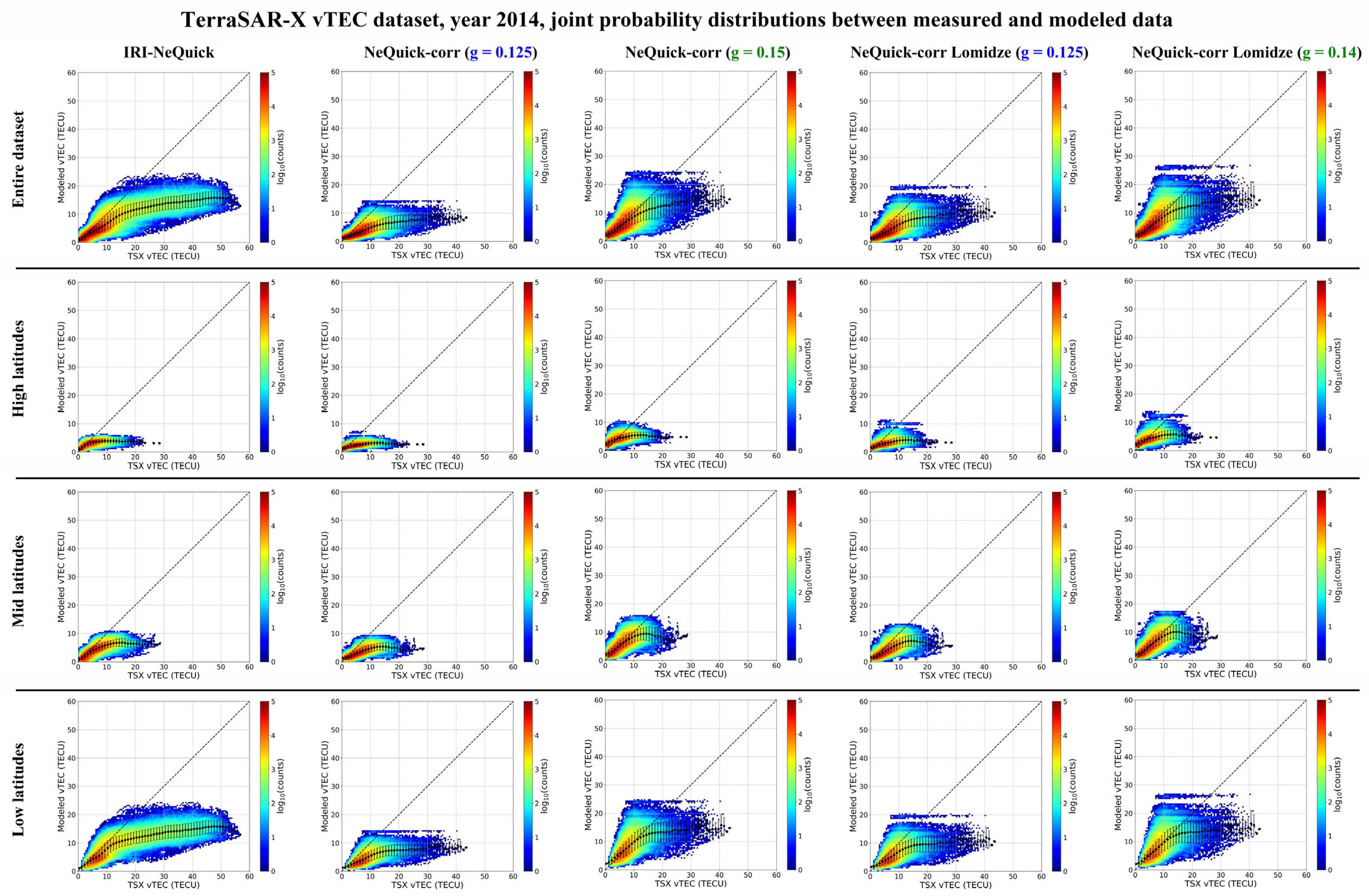
2.5. TerraSAR-X Observations

TerraSAR-X is a radar imaging satellite developed and operated by DLR in collaboration with the Airbus Defence and Space division. Launched on 15 June 2007, TerraSAR-X can acquire high-resolution radar images of the Earth’s surface in a polar orbit at around 515 km of altitude. The satellite payload has no instrument dedicated to the ionospheric research, but it is equipped with a dual-frequency GPS receiver. As shown by Zakharenkova and Cherniak [60], POD data can be effectively used to determine TEC values to properly describe the variabilities of the ionosphere and plasmasphere. vTEC data processed by UCAR for the years 2008, 2011, and 2014 were considered.

2.6. The IRI UP Method

IRI UP [36] is an empirical data assimilation method based on the IRI model. Its aim is the update of the F2-layer description made by the IRI model through the assimilation of foF2 and of the F2-layer propagation factor for a distance of 3000 km, M(3000)F2, routinely recorded by a network of European ionosondes. foF2 is directly related to NmF2 by means of the relation foF2 = (NmF2/(1.24 × 104))1/2, where foF2 and NmF2 are respectively expressed in the units of MHz and el/cm3. These assimilated characteristics are exploited by IRI UP to compute, at each ionosonde location, effective values (IG12eff and R12eff) of IG12 and R12, which are, respectively, the 12-month running-mean of the ionospheric index IG [61] and of the sunspot number R. Starting from these discrete datasets, corresponding effective index maps are generated through the Universal Kriging method [62]. These maps are then used as input for the IRI model to obtain updated values of foF2 and hmF2 over the European region. The IRI UP method proved to be very powerful in obtaining more reliable F2-layer characteristics for both quiet and magnetically disturbed conditions [36,37]. The IRI UP method, assimilating values at a fifteen-minute resolution by twelve European ionosondes (see Table 1 of Pignalberi et al. [36]), outputs updated maps of foF2 and hmF2 over the European region (from 15° W to 45° E in longitude and from 30° N to 60° N in latitude, with a 1° × 1° spatial resolution) every 15 minutes. IRI UP foF2 and hmF2 maps have been calculated for each Swarm satellite’s passage over the European region from 5 December 2013 to 31 December 2021. Ionosonde data were downloaded from the Digital Ionogram DataBASE [63] by means of the SAO Explorer software (https://ulcar.uml.edu/SAO-X/, accessed on 1 April 2024) developed by the University of Massachusetts, Lowell, and are the output of two different autoscaled systems: ARTIST (Automatic Real-Time Ionogram Scaler with True height analysis) [64,65] and Autoscala [66,67]. Specifically, the ARTIST system was applied to autoscale foF2 and M(3000)F2 data from the ionograms recorded by digisondes [68], while Autoscala was applied to autoscale foF2 and M(3000)F2 data from the ionograms recorded by AIS-INGV ionosondes [69] and the VISRC2 ionosonde installed in Warsaw [70].
Pignalberi et al. [37] have improved the first version of the IRI UP method. In addition to considering for the stations equipped with the ARTIST system only ionograms with a Confidence Score [71] greater than 75 [72], they introduced a filter, valid for both ARTIST and Autoscala, to identify wrongly autoscaled ionosonde data and exclude them from the assimilation process. Moreover, they replaced the preliminary quality check used to choose the variogram model in the Universal Kriging method with a new quality check routine (NQCR) based on the variogram’s residuals. NQCR quantitatively identifies the best variogram model used to generate more reliable effective index maps for ingestion in the IRI model to obtain updated foF2 and hmF2 maps. Unlike Pezzopane and Pignalberi [35], whose analyses were based on the first version of IRI UP proposed by Pignalberi et al. [36], in the present study, we applied the IRI UP improvements proposed by Pignalberi et al. [37].

3. The NeQuick Ionospheric Topside Representation and the H0,corr Formulation

NeQuick models the topside ionosphere [16,21] through a semi-Epstein layer describing the electron density as a function of the height h, starting from NmF2 at the hmF2 height
N e ( h ) = 4 N m F 2 exp ( h h m F 2 H ) [ 1 + exp ( h h m F 2 H ) ] 2 ,
where H is a height-dependent empirical scale height
H ( h ) = H 0 [ 1 + r g ( h h m F 2 ) r H 0 + g ( h h m F 2 ) ] ,
with r and g that are constant factors: g = 0.125 is the gradient of H near the F2-layer peak; r = 100 controls the asymptotic behavior of H at infinity. H0 is instead the value of H at hmF2 and is equal to
H 0 = k B 2 bot ,
where B2bot is the NeQuick bottomside thickness parameter [40,41], which represents the scale height of the F2-layer bottomside region; k is defined as
k = 3.22 0.0538 f o F 2 0.00664 h m F 2 + 0.113 h m F 2 B 2 bot + 0.00257 R 12 ;
B2bot is connected to the electron density derivative at the inflection point (dNe(h)/dh)max of the semi-Epstein layer, describing the bottomside F2 layer as follows:
B 2 bot = 0.04774 f o F 2 2 ( d N e ( h ) d h ) max .
Mosert de Gonzales and Radicella [73], using ionosonde data, proposed the following empirical relationship for (dNe(h)/dh)max:
( d N e ( h ) d h ) max = 0.01 exp [ 3.467 + 1.714 ln ( f o F 2 ) + 2.02 ln ( M ( 3000 ) F 2 ) ] .
According to Pezzopane and Pignalberi [35], the main idea behind the development of NeQuick-corr is to obtain corrected values of H0 directly from measurements collected in the topside ionosphere. To accomplish this task, the NeQuick topside Equation (1) is forced to join the F2-layer peak values (hmF2, NmF2), provided by the IRI UP method, and the topside anchor point (hsat, Ne,sat), provided by Swarm satellites. Since the IRI UP method provides F2-layer peak data over the European region at 1° × 1° spatial resolution, Swarm measurements were gridded over the same region, with the same spatial resolution, for each track of satellites over Europe, and for the whole period under study. In particular, to remove any possible outlier for any Swarm satellite passage over Europe, each Ne measurement falling in a 1° × 1° grid point was subjected to the Median Absolute Deviation (MAD) filtering [47,74]. Then, the mean of Ne measurements in each grid point was calculated. These means of Ne represent the topside anchor points (hsat, Ne,sat) considered for the calculation of H0,corr. In the time span considered in this study, the number of tracks cumulated over Europe was 13,293 for Swarm A, 13,092 for Swarm B, and 13,258 for Swarm C. Once gridded at 1° × 1° spatial resolution, the dataset of Ne means consisted of 298,446 values for Swarm A, 295,316 values for Swarm B, and 299,266 values for Swarm C.
A value of H0 is calculated for every couple of co-located and simultaneously measured (by Swarm) and modeled (by IRI UP) anchor points, which gives rise to a huge dataset of H0 over the European region. Due to the temporal resolution of IRI UP maps (fifteen minutes according to the ionosondes’ sounding repetition rate), IRI UP maps and Swarm observations are shifted in time by 7 min and 30 s at most. This time difference is negligible when considering the median climatological behavior of these ionospheric parameters. Computed H0 values are then modeled as a function of foF2 and hmF2, generating for Swarm A and C a joint H0 dataset, taking into account that these satellites fly at the same altitude very close to each other.
Specifically, H0 values are arranged as a function of foF2 and hmF2 by applying the two-dimensional binning procedure described in Pignalberi et al. [75], that is:
  • Each calculated value of H0 is associated to a specific pair of values (foF2, hmF2);
  • H0 values are two-dimensionally binned as a function of foF2 and hmF2, with a bin width of 0.25 MHz and 5 km, respectively, within the following ranges: foF2 ∈ [0, 16] MHz; hmF2 ∈ [150, 450] km;
  • If the number of H0 values in the bin is greater than or equal to 10, the corresponding median is calculated; otherwise, the bin is considered statistically insignificant.
At the end of the analysis, two-dimensional binned grids H0,AC and H0,B of H0, based separately on Swarm A and C measurements and on Swarm B measurements, are generated. The selection of the corresponding H0 value in these two-dimensional grids allows modeling the topside vertical electron density profile through Equations (1) and (2) once a pair of values (foF2, hmF2) is available. It is worth highlighting that this pair of values can be either modeled or measured. Pezzopane and Pignalberi [35] reported a different performance when using the two grids. In particular, they verified that the use of the H0,AC grid gives better results from hmF2 to approximately the Swarm A and C altitude, while the use of the H0,B grid gives better results from the Swarm B altitude to higher ones, and they proposed the following corrected version H0,corr of H0:
{ H 0 , corr = H 0 , AC for h = h m F 2 , H 0 , corr = H 0 , AC + ( H 0 , B H 0 , AC ) h h m F 2 600 for h ( h m F 2 , h m F 2 + 600 ) , H 0 , corr = H 0 , B for h h m F 2 + 600
All the variables in (7) are in km. As it was highlighted by Pezzopane and Pignalberi [35], for the very few bins for which H0,B is lower than or equal to H0,AC, H0,corr is always assumed constant and equal to H0,AC for h > hmF2. Moreover, if for a definite pair (foF2, hmF2) only one value of either H0,AC or H0,B is available, this is assumed to be equal to H0,corr for h > hmF2. The original NeQuick H0 parameter has to be used for those cases for which neither H0,AC nor H0,B is available.
Pezzopane and Pignalberi [35] calculated the two-dimensional binned grids H0,AC and H0,B considering each Swarm satellite’s passage over the European region from 5 December 2013 to 31 December 2018. In this work, we extended the underlying Swarm and IRI UP datasets until 31 December 2021. Moreover, the Swarm calibrated dataset proposed by Lomidze et al. [47] has also been considered.

4. Results and Discussion

Figure 1 shows a comparison between H0,AC and H0,B median values calculated with and without the Lomidze calibration, considering the dataset from 5 December 2013 to 31 December 2018, namely the one used by Pezzopane and Pignalberi [35]. Figure 2 shows the corresponding residuals and percentage residuals. Figure 3 and Figure 4 are the same as Figure 1 and Figure 2 but consider the updated dataset from 5 December 2013 to 31 December 2021.
Figure 1, Figure 2, Figure 3 and Figure 4 show that H0,AC and H0,B values obtained through Lomidze calibrated Ne values are sensibly higher than uncalibrated ones by a factor between 10% and 30%. This is because the Lomidze calibration increased Swarm LP Ne values by a factor depending on the considered Swarm satellite and varying between about 9% and 11% in plasma frequency [47]. Consequently, H0,AC Lomidze and H0,B Lomidze would produce higher Ne values in the topside and then higher vTEC values; this agrees with many past studies that pointed to a general underestimation of vTEC modeled by NeQuick (and then by IRI) (e.g., [35,76]). However, it is worth highlighting that an electron density increase in the topside ionosphere can also be obtained by an increase of the g parameter in the NeQuick topside scale height [32]. This has been recently verified by Singh et al. [46], who pointed out that a value of g = 0.15, instead of 0.125 typically adopted in NeQuick, improves the NeQuick-corr topside representation on a global scale.
On the other hand, Figure 1, Figure 2, Figure 3 and Figure 4 also show that the differences between the H0,AC and H0,B values obtained with the two Ne datasets (from 5 December 2013 to 31 December 2018 and from 5 December 2013 to 31 December 2021) are negligible for most pairs (foF2, hmF2). The largest differences are scattered and visible above all for very low foF2 values, as is well visible in Figure 5, showing the corresponding residuals and percentage residuals.
Once H0,AC and H0,B grids have been calculated, considering as a reference vTEC values recorded by COSMIC-1, GRACE, METOP, TerraSAR-X, and Swarm A satellites, we performed a comparison test of the following five NeQuick topside descriptions:
  • The NeQuick original description (the one represented by Equations (1)−(6)), that until the IRI-2016 version was the default topside option of the IRI model;
  • The NeQuick-corr topside description based on IRI UP modeled values and Swarm uncalibrated Ne measurements from 5 December 2013 to 31 December 2021, considering the value of g = 0.125 typically adopted in NeQuick;
  • The NeQuick-corr topside description based on IRI UP modeled values and Swarm uncalibrated Ne measurements from 5 December 2013 to 31 December 2021, considering g = 0.15 as suggested by Singh et al. [46];
  • The NeQuick-corr topside description based on IRI UP modeled values and Swarm calibrated Ne measurements according to Lomidze et al. [47] from 5 December 2013 to 31 December 2021, considering the value of g = 0.125 typically adopted in NeQuick;
  • The NeQuick-corr topside description based on IRI UP modeled values and Swarm calibrated Ne measurements according to Lomidze et al. [47] from 5 December 2013 to 31 December 2021, considering g = 0.14.
The last topside description is the result of the same analysis described by Singh et al. [46], but this time performed on the NeQuick-corr topside description based on Swarm calibrated Ne measurements. This analysis highlighted how a value of g equal to 0.14, instead of the value 0.125 usually considered by NeQuick, improves the NeQuick-corr topside representation based on Swarm calibrated Ne measurements. It is worth noting that vTEC values from POD antenna observations are representative of the topside ionosphere and plasmasphere electron content, i.e., from the LEO satellite altitude to GNSS altitude (about 20,000 km from the ground).
The comparison test was made considering vTEC data recorded in 2008 (low solar activity, yearly mean value of R12 = 4.2), in 2011 (medium solar activity, yearly mean value of R12 = 73.5), and in 2014 (high solar activity, yearly mean value of R12 = 107.2). The selection of these three years ensured the best possible coverage in terms of satellite data from different missions.
For each dataset, the Root Mean Square Error (RMSE) between modeled and measured vTEC values
RMSE ( TECU ) = i = 1 N ( vTEC modeled , i vTEC measured , i ) 2 N ,
where the index i runs on the N available pairs of modeled and measured vTEC, was calculated by selecting (a) the global dataset, (b) data at high latitudes in the Quasi-Dipole (QD) magnetic latitude [77] range (60° N, 90° N] and (60° S, 90° S], (c) data at middle latitudes in the QD magnetic latitude range (30° N, 60° N] and (30° S, 60° S], and (d) data at low latitudes in the QD magnetic latitude range [30° S, 30° N].
Modeled vTEC values were calculated as follows:
vTEC modeled = h LEO h GNSS = 20 , 000 N e , modeled ( h ) d h ,
where hLEO is the orbit’s altitude of the five LEO satellite missions considered, hGNSS is the orbit’s altitude of the GNSS satellites, and Ne,modeled is the electron density modeled according to the five aforementioned topside descriptions. For each of these, the F2-layer peak anchor point was modeled through the IRI model default options: URSI coefficients for foF2 [78] and the Shubin model for hmF2 [79]. Since the four different NeQuick-corr implementations require a pair (foF2, hmF2) to select a value of both H0,AC and H0,B, only vTEC values associated with (foF2, hmF2) pairs included in the grids shown in Figure 3 have been modeled. Therefore, through the NeQuick-corr formulation, it was impossible to obtain vTEC-modeled values for the whole validation dataset. This issue affects mainly the low latitudes where foF2 and hmF2 values may significantly differ from those recorded over the European region and used to obtain the grids shown in Figure 3.
Table 1 shows a summary of the statistical analysis in terms of RMSE for the year 2014, where the model with the best performance is bolded.
The NeQuick-corr topside description based on IRI UP modeled values and Swarm uncalibrated Ne measurements, from 5 December 2013 to 31 December 2021, considering g = 0.15, proved to be the best model for the majority of cases. Moreover, even in cases where it is not optimal, the performance of the NeQuick-corr (g = 0.15) topside description is very close to the optimal, as in the case of the METOP dataset, for which the best RMSE is obtained by the NeQuick-corr Lomidze (g = 0.14) option. In general, the performance of NeQuick-corr (g = 0.15) is similar to that of NeQuick-corr Lomidze (g = 0.14), which highlights the key role of the g parameter.
Tables related to the years 2008 and 2011 show similar results and are given in the Supplementary Material. Concerning the RMSE values, it is worth highlighting their overall decrease as the solar activity decreases, according to the overall decrease of both measured and modeled vTEC values. Table 1 and those of Supplementary Material show that the results are pretty independent of the latitude and, taking into account that the NeQuick-corr has been developed over the European region, this shows that its analytical description is robust also outside the spatial domain originally considered.
The results reported in Table 1 are complemented with a more in-depth analysis based on joint probability distributions (JPDs) and distributions of residuals between measured and modeled vTEC values. Figure 6 and Figure 7 show the JPDs related to TerraSAR-X and METOP, while Figure 8 and Figure 9 show the corresponding distributions of residuals. Similar plots for GRACE, Swarm A, and COSMIC-1 can be found in the Supplementary Material. In the Supplementary Material, the reader can also find the JPDs and distributions of residuals related to TerraSAR-X, METOP, GRACE, and COSMIC-1 for the years 2008 and 2011.
Figure 6, Figure 7, Figure 8 and Figure 9 show that without modifying the original value of g = 0.125, both the original NeQuick description (i.e., one of the options of the IRI model) and the NeQuick-corr ones significantly underestimate the measurements. Instead, the use of optimized g values (g = 0.15 when considering uncalibrated Swarm Ne values; g = 0.14 when considering calibrated Swarm Ne values according to Lomidze et al. [47]) is very effective and improves the NeQuick-corr performance, reducing significantly the vTEC underestimation. Figure 6, Figure 7, Figure 8 and Figure 9 highlight that the NeQuick-corr (g = 0.15) option shows the best performance, followed by the NeQuick-corr Lomidze (g = 0.14) option.
Most of the improvements concern the accuracy of the NeQuick-corr model, i.e., the mean of the residuals, while the dispersion of data is less affected by the g optimization, as testified by the standard deviation of the residuals. Consequently, the accuracy improvement corresponds to lower RMSE values, which, on the other hand, are far from being close to zero. This fact suggests that the significance of the parameter r, the one controlling the asymptotic behavior of the scale height at infinity, namely in the plasmaspheric domain, cannot be understated. Indeed, our study concerns the optimization of both H0 and g parameters based on data recorded in the first hundreds of kilometers above the F2-layer peak, while a non-negligible fraction of vTEC comes from the plasmasphere where an accurate specification of the r parameter becomes relevant [76]. Pignalberi et al. [80] have recently shown that characterizing globally such parameters through RO observations is not an easy task, especially at low latitudes, and understanding what range of values is to be tested represents a challenge nowadays due to a lack of three-dimensional observations in the ionosphere–plasmasphere transition region. Several recent studies have noted differences in the scale height behavior at the plasmaspheric altitudes compared to the topside ionosphere. For instance, Prol et al. [7] performed a statistical analysis of the scale height using topside sounder observations. They found a notable transition from an approximately linear dependence of the scale height on altitude to the parabolic one at around 1000–1500 km heights. Furthermore, Prol et al. [30] found that using Van Allen Probes data, specifically Ne measurements near the plasmapause, improved our understanding of the plasmasphere. These data could be valuable for future studies focused on tracking variations of the r parameter and might likely lead to a reduction of VTEC residuals shown in Figure 8 and Figure 9.
Another feature that stands out from Figure 8 is that at high latitudes, the distribution of residuals of TerraSAR-X shows a double-hump structure when the NeQuick-corr is considered without optimizing the parameter g. The optimization of the parameter g somehow smooths out this feature. The same holds for Swarm A and GRACE, but not for COSMIC-1 and METOP (see also the Supplementary Material). A possible cause of this behavior is that the analyses have been done without performing any local time and seasonal sorting, and this at high latitudes might have triggered such a double hump structure. The investigation of this particular behavior at high latitudes is, however, out of the scope of the present study.
According to Pezzopane and Pignalberi [35], an additional analysis that has been done is based on COSMIC-1 RO electron density profiles from April 2006 to December 2018. For each RO profile, vTEC is calculated by integrating the topside electron density values from hmF2 to 600 km above hmF2, as follows:
vTEC measured = h m F 2 h m F 2 + 600 N e , COS MIC 1 ( h ) d h .
Moreover, each RO electron density profile provides measured values of foF2 and hmF2 that are used to model the IRI-NeQuick and the four NeQuick-corr topside profiles considered in this study. vTEC modeled values are then calculated as follows:
vTEC modeled = h m F 2 h m F 2 + 600 N e , modeled ( h ) d h
In this way, vTECmodeled values and vTECmeasured values are based on the same F2-layer peak anchor point. With this analysis, the performance of the models is evaluated for the lowest topside section, i.e., where the correction is believed to be most effective, as it is based on Swarm data recorded in the altitude range of 460–520 km. Moreover, this analysis highlights a possible solar activity dependence effect on models’ performance, something that the RMSE values shown in Table 1 and in those of the Supplementary Material seem to testify.
Figure 10, Figure 11 and Figure 12 show the yearly mean of RMSE values calculated between modeled and measured vTEC values respectively for: Northern high latitudes, for QD magnetic latitudes above 60° N; Northern middle latitudes, for QD magnetic latitudes between 30° N and 60° N; low latitudes, for QD magnetic latitudes between 30° S and 30° N. Pezzopane and Pignalberi [35] performed such an analysis only for middle latitudes.
Figures related to Southern high and middle latitudes show similar results as the Northern hemisphere and can be found in the Supplementary Material.
Figure 10, Figure 11 and Figure 12 highlight that the performance of the models shows a rather marked dependence on solar activity, with the RMSE values increasing as the solar activity increases. Even more significant, the performance among different models presents a different dependence on solar activity variations. For example, at middle latitudes, the Lomidze calibration produces worse results for low solar activity and better results for high solar activity when compared to uncalibrated Ne values.
At high latitudes, the NeQuick-corr description, in most cases, cannot improve the IRI-NeQuick performance. This is rather expected, being the NeQuick-corr formulation based on data recorded over the European region. On the other hand, this is something that seems to be restricted to the lowest topside section because Table 1 and those of the Supplementary Material showed that the NeQuick-corr model performs reasonably well also at high latitudes. Concerning the low latitudes, this analysis confirms that, although the NeQuick-corr is based on data recorded over the European region, its performance is generally good, even though, in this case, both the Lomidze calibration and the optimization of the g value do not bring any improvement. This outcome might be ascribed to the restriction of this analysis to vTEC values from hmF2 to 600 km.

5. Summary and Conclusions

This study is a continuation of the work by Pezzopane and Pignalberi [35]. The numerical grids of H0,corr were updated by extending the underlying Swarm and IRI UP datasets until December 2021. The extension of the dataset facilitated coverage of low solar activity conditions that were not considered before. In addition, regarding Swarm measurements, it also considered the calibration proposed by Lomidze et al. [47]. Correspondingly, two different sets of grids of H0,corr have been calculated and tested. The test has been made globally for low, middle, and high latitudes, considering both vTEC values measured by POD antennas and those obtained by integrating the RO profiles recorded by LEO satellites. The main outcomes of the study can be summarized as follows:
  • Even though the NeQuick-corr formulation is based on datasets recorded over the European region, its performance is deemed satisfactory for both low, middle, and high latitudes when considering the profile up to the GNSS satellites’ altitude. On the other hand, when considering the lowest topside section, from hmF2 to 600 km above hmF2, it was demonstrated that NeQuick-corr provides adequate performance at low and middle latitudes;
  • The study highlighted that considering values of the parameter g other than 0.125 (usually adopted) is very effective in mitigating the vTEC underestimation made by the NeQuick model and significantly improves the NeQuick-corr performance, primarily in terms of accuracy;
  • The best performance is obtained by the NeQuick-corr topside description corresponding to g = 0.15 and by the NeQuick-corr Lomidze topside description corresponding to g = 0.14;
  • RMSE deviates significantly from 0. This fact suggests that the significance of parameter r, which controls the asymptotic behavior in the plasmaspheric domain, is crucial, and its modeling becomes a necessity for an accurate vTEC modeling;
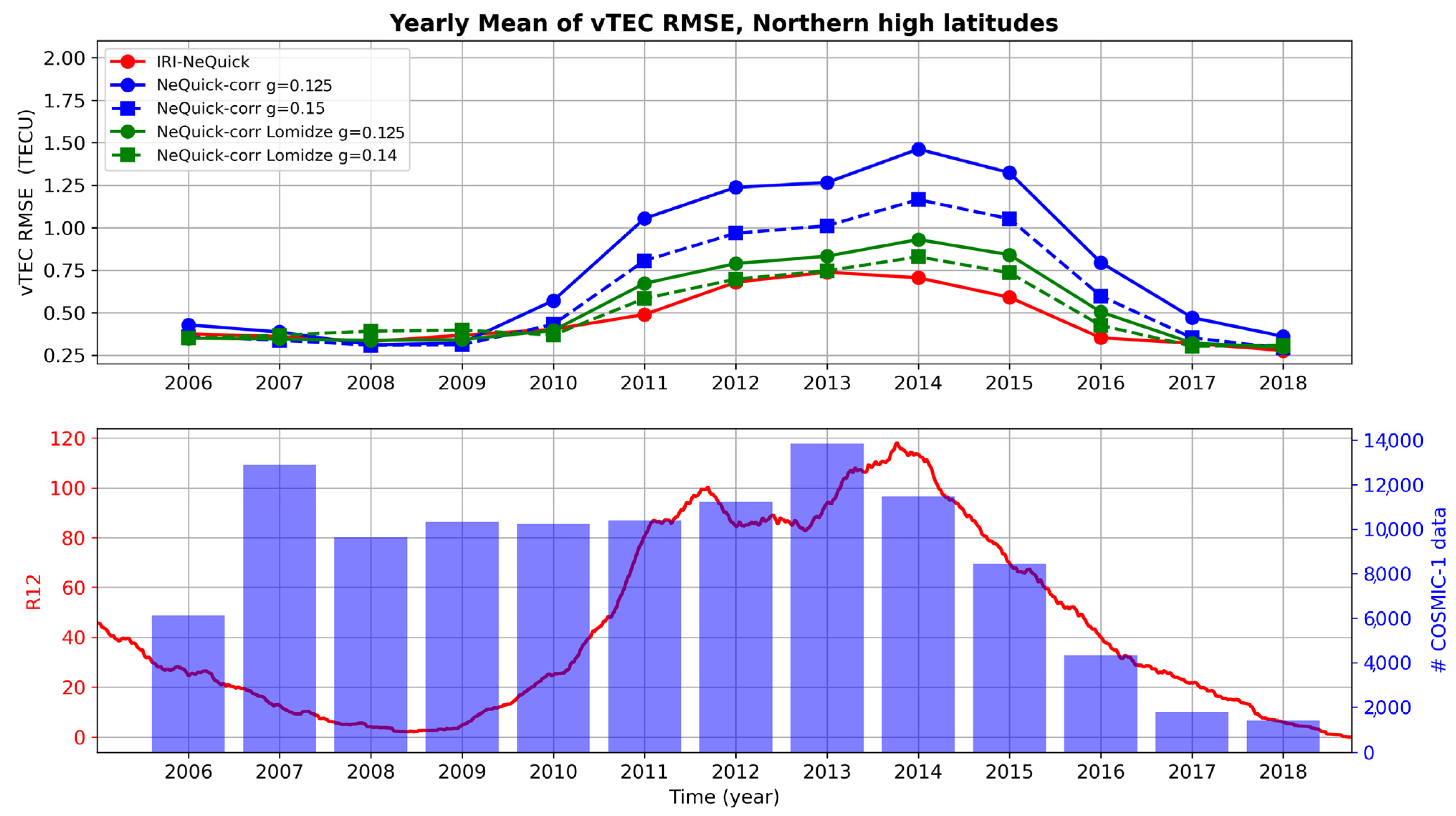
  • The performance of different NeQuick-corr options depends on solar activity, with the RMSE increasing as the solar activity increases. This feature is smoothed out when considering optimized values of g. This suggests that the g parameter is most likely dependent on the solar activity level. In fact, especially at middle latitudes, the application of the optimized g parameter is very effective for high but not for low solar activity years. On the other hand, Pignalberi et al. [80] have recently highlighted this dependence.
While Lomidze-calibrated Ne values are currently considered as the nominal Swarm LP Ne dataset, recent investigations by Smirnov et al. [81], Xiong et al. [82], Pignalberi et al. [83] and Haralambous et al. [84] pointed out how Swarm LP Ne values exhibit local time and solar activity variations that were not described by the Lomidze et al. [47] calibration procedure. In particular, it has been recently demonstrated that the Swarm LPs overestimate the plasma densities on the nightside at low and middle latitudes. This is due to an assumption made in the ion densities calculation that the ambient plasma consists exclusively of O+ ions, which is frequently violated at nighttime during low solar activity [81,82]. Therefore, in the future, the calculation of H0 values through Swarm LP observations could be further refined by applying the recommendation resulting from the Swarm LP calibration and validation ongoing process.
The results of the study highlight the need for a revision of the original NeQuick topside formulation (used also by the IRI model). The link of H0 with the bottomside, included in the NeQuick-corr formulation, could be abandoned, but also the constant values of g and r should be critically evaluated. Anyhow, our results suggest the use of the NeQuick-corr formulation, instead of the original one, when modeling the topside from hmF2 to the GNSS altitude.

Supplementary Materials

The following supporting information can be downloaded at https://www.mdpi.com/article/10.3390/atmos15040498/s1, Figures S1–S26; Tables S1 and S2.

Author Contributions

Conceptualization, A.P., M.P. (Michael Pezzopane); methodology, A.P., M.P. (Michael Pezzopane); data curation and formal analysis, A.P., H.H. and F.P.; investigation, all authors; writing—original draft preparation, M.P. (Michael Pezzopane); writing—review and editing, all authors. All authors have read and agreed to the published version of the manuscript.

Funding

This research received no external funding.

Institutional Review Board Statement

Not applicable.

Informed Consent Statement

Not applicable.

Data Availability Statement

Data from ionospheric observatories are available via the public access portal of the Digital Ionogram Database (https://giro.uml.edu/didbase/, accessed on 31 January 2024) of the Global Ionosphere Radio Observatory in Lowell, MA. ESA Swarm data are publicly available at https://swarm-diss.eo.esa.int/ (accessed on 31 January 2024). COSMIC—1 RO data are stored in the COSMIC Data Analysis and Archive Center (CDAAC, http://cdaac-www.cosmic.ucar.edu/cdaac/products.html, accessed on 31 January 2024). vTEC values of GRACE, METOP, TerraSAR-X are freely available through the Database for Ionospheric Model Evaluation website https://sites.google.com/view/ionodime/experiments/topiono-plasmasphere (accessed on 31 January 2024).

Acknowledgments

This publication uses data from ionospheric observatories made available via the public access portal of the Digital Ionogram Database (https://giro.uml.edu/didbase/, accessed on 31 January 2024) of the Global Ionosphere Radio Observatory in Lowell, MA. The authors are indebted to the observatory directors and ionosonde operators for the significant investments of their time, effort, expertise, and funds needed to acquire and provide measurement data for academic research. The IRI team is acknowledged for developing and maintaining the IRI model and for giving access to the corresponding Fortran code via the IRI Web site (http://irimodel.org/, accessed on 1 April 2024). The authors thank the Telecommunications/ICT for Development (T/ICT4D) Laboratory Team, The Abdus Salam International Centre for Theoretical Physics, Trieste, Italy, for developing, maintaining, and making available the NeQuick model (https://t-ict4d.ictp.it/nequick2/nequick-2-web-model, accessed on 1 April 2024). Thanks are due to the COSMIC/FORMOSAT-3 team for making freely available radio occultation data by means of the COSMIC Data Analysis and Archive Center (CDAAC, http://cdaac-www.cosmic.ucar.edu/cdaac/products.html, accessed on 1 April 2024) and to the Swarm team for making freely available data from https://swarm-diss.eo.esa.int/. Haris Haralambous’s contribution was partially funded by the project “International Reference Ionosphere Validation and Improvement”—IRIVM (Ref. No: EXCELLENCE/0421/0422) that was co-funded by the Republic of Cyprus and the European Regional Development Fund (ERDF), in the frame of the Operational Programme “ΘAλΕΙA” 2021–2027 under Priority 1: “Competitive, Smart and Digital Economy” and the Specific Objective (1i): “Developing and enhancing research and innovation capacities and the uptake of advanced technologies”.

Conflicts of Interest

The authors declare no conflicts of interest.

References

  1. Rishbeth, H.; Garriott, O. Introduction to ionospheric physics. In International Geophysics Series; Academic Press: New York, NY, USA, 1969; Volume 14. [Google Scholar]
  2. Yizengaw, E.; Moldwin, M.B.; Galvan, D.; Iijima, B.A.; Komjathy, A.; Mannucci, A.J. Global plasmaspheric TEC and its relative contribution to GPS TEC. J. Atmos. Sol.-Terr. Phys. 2008, 70, 1541–1548. [Google Scholar] [CrossRef]
  3. Hoque, M.M.; Jakowski, N. Ionospheric propagation effects on GNSS signals and new correction approaches. In Global Navigation Satellite Systems; Jin, S., Ed.; IntechOpen: Rijeka, Croatia, 2012; Chapter 16; pp. 381–405. [Google Scholar] [CrossRef]
  4. Olivares-Pulido, G.; Hernández-Pajares, M.; Aragón-Àngel, A.; Garcia-Rigo, A. A linear scale height chapman model supported by GNSS occultation measurements. J. Geophys. Res. Space Phys. 2016, 121, 7932–7940. [Google Scholar] [CrossRef]
  5. Radicella, S.M.; Nava, B.; Coïsson, P. Ionospheric Models for GNSS Single Frequency Range Delay Corrections. Física Tierra 2008, 20, 27–39. [Google Scholar]
  6. dos Santos Prol, F.; Hernández-Pajares, M.; de Oliveira Camargo, P.; de Assis Honorato Muella, M.T. Spatial and temporal features of the topside ionospheric electron density by a new model based on GPS radio occultation data. J. Geophys. Res. Space Phys. 2018, 123, 2104–2115. [Google Scholar] [CrossRef]
  7. dos Santos Prol, F.; Themens, D.R.; Hernández-Pajares, M.; de Oliveira Camargo, P.; de Assis Honorato Muella, M.T. Linear vary-chap topside electron density model with topside sounder and radio-occultation data. Surv. Geophys. 2019, 40, 277–293. [Google Scholar] [CrossRef]
  8. Habarulema, J.B.; Okoh, D.; Bergeot, N.; Burešová, D.; Matamba, T.; Tshisaphungo, M.; Katamzi-Joseph, Z.; Pinat, E.; Chevalier, J.-M.; Seemala, G. Interhemispheric comparison of the ionosphere and plasmasphere total electron content using GPS, radio occultation and ionosonde observations. Adv. Space Res. 2021, 68, 2339–2353. [Google Scholar] [CrossRef]
  9. Park, J. Ratio between over satellite electron content and plasma density measured by Swarm: A proxy for topside scale height. J. Geophys. Res. Space Phys. 2022, 127, e2021JA030137. [Google Scholar] [CrossRef]
  10. Ren, X.; Li, Y.; Mei, D.; Zhu, W.; Zhang, X. Improving topside ionospheric empirical model using FORMOSAT-7/COSMIC-2 data. J. Geodesy 2023, 97, 30. [Google Scholar] [CrossRef]
  11. Kuverova, V.V.; Adamson, S.O.; Berlin, A.A.; Bychkov, V.L.; Dmitriev, A.V.; Dyakov, Y.A.; Eppelbaum, L.V.; Golubkov, G.V.; Lushnikov, A.A.; Manzhelii, M.I.; et al. Chemical physics of D and E layers of the ionosphere. Adv. Space Res. 2019, 64, 1876–1886. [Google Scholar] [CrossRef]
  12. Hunsucker, R.D. Radio Techniques for Probing the Terrestrial Ionosphere; Springer: Berlin/Heidelberg, Germany, 1991. [Google Scholar] [CrossRef]
  13. Bilitza, D.; Pezzopane, M.; Truhlik, V.; Altadill, D.; Reinisch, B.W.; Pignalberi, A. The International Reference Ionosphere model: A review and description of an ionospheric benchmark. Rev. Geophys. 2022, 60, e2022RG000792. [Google Scholar] [CrossRef]
  14. Bilitza, D.; Reinisch, B.W.; Radicella, S.M.; Pulinets, S.; Gulyaeva, T.; Triskova, L. Improvements of the International Reference Ionosphere model for the topside electron density profile. Radio Sci. 2006, 41, RS5S15. [Google Scholar] [CrossRef]
  15. Coïsson, P.; Radicella, S.M. Ionospheric topside models compared with experimental electron density profiles. Ann. Geophys. 2005, 48, 497–503. [Google Scholar] [CrossRef]
  16. Coïsson, P.; Radicella, S.M.; Leitinger, R.; Nava, B. Topside electron density in IRI and NeQuick: Features and limitations. Adv. Space Res. 2006, 37, 937–942. [Google Scholar] [CrossRef]
  17. Lühr, H.; Xiong, C. The IRI 2007 model overestimates electron density during the 23/24 solar minimum. Geophys. Res. Lett. 2010, 37, L23101. [Google Scholar] [CrossRef]
  18. Pignalberi, A.; Pezzopane, M.; Tozzi, R.; De Michelis, P.; Coco, I. Comparison between IRI and preliminar Swarm Langmuir probe measurements during the St. Patrick storm period. Earth Planets Space 2016, 68, 93. [Google Scholar] [CrossRef]
  19. Leitinger, R.; Nava, B.; Hochegger, G.; Radicella, S. Ionospheric profilers using data grids. Phys. Chem. Earth Part C Solar Terr. Plan. Sci. 2001, 26, 293–301. [Google Scholar] [CrossRef]
  20. Leitinger, R.; Radicella, S.; Hochegger, G.; Nava, B. Diffusive equilibrium models for the height region above the F2 peak. Adv. Space Res. 2002, 29, 809–814. [Google Scholar] [CrossRef]
  21. Nava, B.; Coïsson, P.; Radicella, S.M. A new version of the NeQuick ionosphere electron density model. J. Atmos. Sol.-Terr. Phys. 2008, 70, 1856–1862. [Google Scholar] [CrossRef]
  22. Coïsson, P.; Nava, B.; Radicella, S.M. On the use of NeQuick topside option in IRI-2007. Adv. Space Res. 2009, 43, 1688–1693. [Google Scholar] [CrossRef]
  23. Radicella, S.M.; Leitinger, R. The evolution of the DGR approach to model electron density profiles. Adv. Space Res. 2001, 27, 35–40. [Google Scholar] [CrossRef]
  24. Chapman, S. The absorption and dissociative or ionizing effect of monochromatic radiation in an atmosphere on a rotating Earth. Proc. Phys. Soc. 1931, 43, 26–45. [Google Scholar] [CrossRef]
  25. Rawer, K. Synthesis of ionospheric electron density profiles with Epstein functions. Adv. Space Res. 1988, 8, 191–199. [Google Scholar] [CrossRef]
  26. Pignalberi, A.; Pezzopane, M.; Nava, B.; Coïsson, P. On the link between the topside ionospheric effective scale height and the plasma ambipolar diffusion, theory and preliminary results. Sci. Rep. 2020, 10, 17541. [Google Scholar] [CrossRef] [PubMed]
  27. Reinisch, B.W.; Nsumei, P.; Huang, X.; Bilitza, D. Modeling the F2 topside and plasmasphere for IRI using IMAGE/RPI and ISIS data. Adv. Space Res. 2007, 39, 731–738. [Google Scholar] [CrossRef]
  28. Nsumei, P.; Reinisch, B.W.; Huang, X.; Bilitza, D. New Vary-Chap profile of the topside ionosphere electron density distribution for use with the IRI model and the GIRO real time data. Radio Sci. 2012, 47, RS0L16. [Google Scholar] [CrossRef]
  29. Hernández-Pajares, M.; Garcia-Fernàndez, M.; Rius, A.; Notarpietro, R.; von Engeln, A.; Olivares-Pulido, G.; Aragón-Àngel, À.; García-Rigo, A. Electron density extrapolation above F2 peak by the linear Vary-Chap model supporting new Global Navigation Satellite Systems-LEO occultation missions. J. Geophys. Res. Space Phys. 2017, 122, 9003–9014. [Google Scholar] [CrossRef]
  30. Prol, F.d.S.; Smirnov, A.G.; Hoque, M.M.; Shprits, Y.Y. Combined model of topside ionosphere and plasmasphere derived from radio-occultation and Van Allen Probes data. Sci. Rep. 2022, 12, 9732. [Google Scholar] [CrossRef] [PubMed]
  31. Smirnov, A.; Shprits, Y.; Prol, F.; Lühr, H.; Berrendorf, M.; Zhelavskaya, I.; Xiong, C. A novel neural network model of Earth’s topside ionosphere. Sci. Rep. 2023, 13, 1303. [Google Scholar] [CrossRef] [PubMed]
  32. Pignalberi, A.; Pezzopane, M.; Themens, D.R.; Haralambous, H.; Nava, B.; Coïsson, P. On the analytical description of the topside ionosphere by NeQuick: Modeling the scale height through COSMIC/FORMOSAT-3 selected data. IEEE J. Sel. Top. Appl. Earth Observ. Remote Sens. 2020, 13, 1867–1878. [Google Scholar] [CrossRef]
  33. Themens, D.R.; Jayachandran, P.T.; Bilitza, D.; Erickson, P.J.; Häggström, I.; Lyashenko, M.V.; Reid, B.; Varney, R.H.; Pustovalova, L. Topside electron density representations for middle and high latitudes: A topside parameterization for E-CHAIM based on the NeQuick. J. Geophys. Res. Space Phys. 2018, 123, 1603–1617. [Google Scholar] [CrossRef]
  34. Bauer, S.J. Diffusive equilibrium in the topside ionosphere. Proc. IEEE 1969, 57, 1114–1118. [Google Scholar] [CrossRef]
  35. Pezzopane, M.; Pignalberi, A. The ESA Swarm mission to help ionospheric modeling: A new NeQuick topside formulation for mid-latitude regions. Sci. Rep. 2019, 9, 12253. [Google Scholar] [CrossRef] [PubMed]
  36. Pignalberi, A.; Pezzopane, M.; Rizzi, R.; Galkin, I. Effective solar indices for ionospheric modeling: A review and a proposal for a real-time regional IRI. Surv. Geophys. 2018, 39, 125–167. [Google Scholar] [CrossRef]
  37. Pignalberi, A.; Pietrella, M.; Pezzopane, M.; Rizzi, R. Improvements and validation of the IRI UP method under moderate, strong, and severe geomagnetic storms. Earth Planets Space 2018, 70, 180. [Google Scholar] [CrossRef]
  38. Friis-Christensen, E.; Lühr, H.; Hulot, G. Swarm: A constellation to study the Earth’s magnetic field. Earth Planets Space 2006, 58, 351–358. [Google Scholar] [CrossRef]
  39. Friis-Christensen, E.; Lühr, H.; Knudsen, D.; Haagmans, R. Swarm—An Earth Observation Mission investigating Geospace. Adv. Space Res. 2008, 41, 210–216. [Google Scholar] [CrossRef]
  40. Leitinger, R.; Zhang, M.L.; Radicella, S.M. An improved bottomside for the ionospheric electron density model NeQuick. Ann. Geophys. 2005, 48, 525–534. [Google Scholar] [CrossRef]
  41. Radicella, S.M.; Alazo-Cuartas, K.; Migoya-Orué, Y.; Kashcheyev, A. Thickness parameters in the empirical modeling of bottomside electron density profiles. Adv. Space Res. 2021, 68, 2069–2075. [Google Scholar] [CrossRef]
  42. Themens, D.R.; Jayachandran, P.T.; Varney, R.H. Examining the use of the NeQuick bottomside and topside parameterizations at high latitudes. Adv. Space Res. 2018, 61, 287–294. [Google Scholar] [CrossRef]
  43. Pezzopane, M.; Pignalberi, A.; Nava, B. On the low-latitude NeQuick topside ionosphere mismodelling: The role of parameters H0, g, and r. Adv. Space Res. 2023, 72, 1224–1236. [Google Scholar] [CrossRef]
  44. Singh, A.K.; Haralambous, H.; Oikonomou, C.; Leontiou, T. A topside investigation over a mid-latitude digisonde station in Cyprus. Adv. Space Res. 2021, 67, 739–748. [Google Scholar] [CrossRef]
  45. dos Santos Klipp, T.; Petry, A.; de Souza, J.R.; de Paula, E.R.; Falcão, G.S.; de Campos Velho, H.F. Ionosonde total electron content evaluation using International Global Navigation Satellite System Service data. Ann. Geophys. 2020, 38, 347–357. [Google Scholar] [CrossRef]
  46. Singh, A.K.; Haralambous, H.; Oikonomou, C. Validation and improvement of NeQuick topside ionospheric formulation using COSMIC/FORMOSAT-3 data. J. Geophys. Res. Space Phys. 2021, 126, e2020JA028720. [Google Scholar] [CrossRef]
  47. Lomidze, L.; Knudsen, D.J.; Burchill, J.; Kouznetsov, A.; Buchert, S.C. Calibration and validation of Swarm plasma densities and electron temperatures using ground-based radars and satellite radio occultation measurements. Radio Sci. 2018, 53, 15–36. [Google Scholar] [CrossRef]
  48. Catapano, F.; Buchert, S.; Qamili, E.; Nilsson, T.; Bouffard, J.; Siemes, C.; Coco, I.; D’Amicis, R.; Tøffner-Clausen, L.; Trenchi, L.; et al. Swarm Langmuir probes’ data quality validation and future improvements. Geosci. Instrum. Method. Data Syst. 2022, 11, 149–162. [Google Scholar] [CrossRef]
  49. Knudsen, D.J.; Burchill, J.K.; Buchert, S.C.; Eriksson, A.I.; Gill, R.; Wahlund, J.; Åhlen, L.; Smith, M.; Moffat, B. Thermal ion imagers and Langmuir probes in the Swarm electric field instruments. J. Geophys. Res. Space Phys. 2017, 122, 2655–2673. [Google Scholar] [CrossRef]
  50. Swarm L1b Product Definition. Available online: https://earth.esa.int/eogateway/documents/20142/37627/swarm-level-1b-product-definition-specification.pdf (accessed on 31 January 2024).
  51. Van den IJssel, J.; Forte, B.; Montenbruck, O. Impact of Swarm GPS receiver updates on POD performance. Earth Planets Space 2016, 68, 85. [Google Scholar] [CrossRef]
  52. Swarm L2 TEC Product Description. Available online: https://earth.esa.int/eogateway/documents/20142/37627/swarm-level-2-tec-product-description.pdf/8fe7fa04-6b4f-86a7-5e4c-99bb280ccc7e (accessed on 31 January 2024).
  53. Anthes, R.; Bernhardt, P.A.; Chen, Y.; Cucurull, L.; Dymond, K.F.; Ector, D.; Healy, S.B.; Ho, S.-P.; Hunt, D.C.; Kuo, Y.-H.; et al. The COSMIC/FORMOSAT-3 mission: Early results. Bull. Am. Meteorol. Soc. 2008, 89, 313–333. [Google Scholar] [CrossRef]
  54. UCAR/NCAR—COSMIC. UCAR COSMIC Program. COSMIC-1 Data Products [IonPrf and podTec]. 2022. Available online: https://www.cosmic.ucar.edu/what-we-do/cosmic-1/data (accessed on 1 April 2024). [CrossRef]
  55. Foelsche, U.; Kirchengast, G. A simple ‘geometric’ mapping function for the hydrostatic delay at radio frequencies and assessment of its performance. Geophys. Res. Lett. 2002, 29, 1473. [Google Scholar] [CrossRef]
  56. Zhong, J.; Lei, J.; Dou, X.; Yue, X. Assessment of vertical TEC mapping functions for space-based GNSS observations. GPS Sol. 2016, 20, 353–362. [Google Scholar] [CrossRef]
  57. Prol, F.S.; Hoque, M.M. A Tomographic Method for the Reconstruction of the Plasmasphere Based on COSMIC/FORMOSAT-3 Data. IEEE J. Sel. Top. Appl. Earth Obs. Remote Sens. 2022, 15, 2197–2208. [Google Scholar] [CrossRef]
  58. von Engeln, A.; Andres, Y.; Marquardt, C.; Sancho, F. GRAS radio occultation on-board of Metop. Adv. Space Res. 2011, 47, 336–347. [Google Scholar] [CrossRef]
  59. Prol, F.S.; Hoque, M.M.; Hernández-Pajares, M.; Yuan, L.; Olivares-Pulido, G.; von Engeln, A.; Marquardt, C.; Notarpietro, R. Study of Ionospheric Bending Angle and Scintillation Profiles Derived by GNSS Radio-Occultation with MetOp-A Satellite. Remote Sens. 2023, 15, 1663. [Google Scholar] [CrossRef]
  60. Zakharenkova, I.; Cherniak, I. How can GOCE and TerraSAR-X contribute to the topside ionosphere and plasmasphere research? Space Weather 2015, 13, 271–285. [Google Scholar] [CrossRef]
  61. Liu, R.Y.; Smith, P.A.; King, J.W. A new solar index which leads to improved foF2 predictions using the CCIR Atlas. Telecommun. J. 1983, 50, 408–414. [Google Scholar]
  62. Kitanidis, P.K. Introduction to Geostatistics: Application to Hydrogeology; Cambridge University Press: Cambridge, UK, 1997. [Google Scholar]
  63. Reinisch, B.W.; Galkin, I.A. Global Ionospheric Radio Observatory (GIRO). Earth Planets Space 2011, 63, 377–381. [Google Scholar] [CrossRef]
  64. Reinisch, B.W.; Huang, X. Automatic calculation of electron density profiles from digital ionograms: 3. Processing of bottomside ionograms. Radio Sci. 1983, 18, 477–492. [Google Scholar] [CrossRef]
  65. Galkin, I.A.; Reinisch, B.W. The New ARTIST 5 for All Digisondes. Ionosonde Network Advisory Group Bulletin 69. 2008. Available online: https://www.sws.bom.gov.au/IPSHosted/INAG/web-69/2008/artist5-inag.pdf (accessed on 1 April 2024).
  66. Scotto, C.; Pezzopane, M. Removing multiple reflections from the F2 layer to improve Autoscala performance. J. Atmos. Sol.-Terr. Phys. 2008, 70, 1929–1934. [Google Scholar] [CrossRef]
  67. Pezzopane, M.; Scotto, C. Highlighting the F2 trace on an ionogram to improve Autoscala performance. Comp. Geosci. 2010, 36, 1168–1177. [Google Scholar] [CrossRef]
  68. Bibl, K.; Reinisch, B.W. The universal digital ionosonde. Radio Sci. 1978, 13, 519–530. [Google Scholar] [CrossRef]
  69. Zuccheretti, E.; Tutone, G.; Sciacca, U.; Bianchi, C.; Arokiasamy, B.J. The new AIS-INGV digital ionosonde. Ann. Geophys. 2003, 46, 647–659. [Google Scholar] [CrossRef]
  70. Pezzopane, M.; Scotto, C.; Tomasik, Ł.; Krasheninnikov, I. Autoscala: An aid for different ionosondes. Acta Geophys. 2009, 58, 513–526. [Google Scholar] [CrossRef]
  71. Galkin, I.A.; Reinisch, B.W.; Huang, X.; Khmyrov, G.M. Confidence score of ARTIST-5 ionogram autoscaling. In Ionosonde Network Advisory Group (INAG) Bulletin, 73rd ed.; International Radio Science Union: Ghent, Belgium, 2013; Available online: http://www.ursi.org/files/CommissionWebsites/INAG/web-73/confidence_score.pdf (accessed on 31 January 2024).
  72. Themens, D.; Reid, B.; Elvidge, S. ARTIST ionogram autoscaling confidence scores: Best practices. URSI Radio Sci. Lett. 2022, 4, 1–5. [Google Scholar] [CrossRef]
  73. Mosert de Gonzales, M.; Radicella, S.M. On a characteristic point at the base of F2 layer in the ionosphere. Adv. Space Res. 1990, 10, 17–25. [Google Scholar] [CrossRef]
  74. Huber, P.J.; Ronchetti, E.M. Robust Statistics; John Wiley & Sons: Hoboken, NJ, USA, 2009. [Google Scholar]
  75. Pignalberi, A.; Pezzopane, M.; Rizzi, R. Modeling the lower part of the topside ionospheric vertical electron density profile over the European region by means of Swarm satellites data and IRI UP method. Space Weather 2018, 16, 304–320. [Google Scholar] [CrossRef]
  76. Kashcheyev, A.; Nava, B. Validation of NeQuick 2 model topside ionosphere and plasmasphere electron content using COSMIC POD TEC. J. Geophys. Res. Space Phys. 2019, 124, 9525–9536. [Google Scholar] [CrossRef]
  77. Laundal, K.M.; Richmond, A.D. Magnetic Coordinate Systems. Space Sci. Rev. 2017, 206, 27. [Google Scholar] [CrossRef]
  78. Rush, C.M.; Fox, M.; Bilitza, D.; Davies, K.; McNamara, L.; Stewart, F.G.; PoKempner, M. Ionospheric mapping-an update of foF2 coefficients. Telecommun. J. 1989, 56, 179–182. [Google Scholar]
  79. Shubin, V.N. Global median model of the F2-layer peak height based on ionospheric radio-occultation and ground based digisonde observations. Adv. Space Res. 2015, 56, 916–928. [Google Scholar] [CrossRef]
  80. Pignalberi, A.; Pezzopane, M.; Nava, B. Optimizing the NeQuick topside scale height parameters through COSMIC/FORMOSAT-3 radio occultation data. IEEE Geosci. Remote Sens. Lett. 2022, 19, 8017005. [Google Scholar] [CrossRef]
  81. Smirnov, A.; Shprits, Y.; Zhelavskaya, I.; Lühr, H.; Xiong, C.; Goss, A.; Prol, F.S.; Schmidt, M.; Hoque, M.; Pedatella, N.; et al. Intercalibration of the plasma density measurements in Earth’s topside ionosphere. J. Geophys. Res. Space Phys. 2021, 126, e2021JA029334. [Google Scholar] [CrossRef]
  82. Xiong, C.; Jiang, H.; Yan, R.; Lühr, H.; Stolle, C.; Yin, F.; Smirnov, A.; Piersanti, M.; Liu, Y.; Wan, X.; et al. Solar flux influence on the in-situ plasma density at topside ionosphere measured by Swarm satellites. J. Geophys. Res. Space Phys. 2022, 127, e2022JA030275. [Google Scholar] [CrossRef]
  83. Pignalberi, A.; Pezzopane, M.; Coco, I.; Piersanti, M.; Giannattasio, F.; De Michelis, P.; Tozzi, R.; Consolini, G. Inter-Calibration and Statistical Validation of Topside Ionosphere Electron Density Observations Made by CSES—01 Mission. Remote Sens. 2022, 14, 4679. [Google Scholar] [CrossRef]
  84. Haralambous, H.; Paul, K.S.; Singh, A.K.; Gulyaeva, T. Investigation of the Topside Ionosphere over Cyprus and Russia Using Swarm Data. Remote Sens. 2023, 15, 1344. [Google Scholar] [CrossRef]
Figure 1. Median values of (top) H0,AC and (bottom) H0,B, as a function of foF2 and hmF2, calculated by using the NeQuick topside formulation, the IRI UP modeled values and Swarm (left) uncalibrated and (right) calibrated electron density measurements according to Lomidze et al. [47], from 5 December 2013 to 31 December 2018. Corresponding plots of occurrences of values in each bin are given in the Supplementary Material.
Atmosphere 15 00498 g001
Figure 2. (Left) Residuals and (right) percentage residuals between median values of (top) H0,AC and (bottom) H0,B calculated considering Swarm uncalibrated and calibrated electron density measurements according to Lomidze et al. [47], from 5 December 2013 to 31 December 2018.
Atmosphere 15 00498 g002
Figure 3. Median values of (top) H0,AC and (bottom) H0,B, as a function of foF2 and hmF2, calculated by using the NeQuick topside formulation, the IRI UP modeled values and Swarm (left) uncalibrated and (right) calibrated electron density measurements according to Lomidze et al. [47], from 5 December 2013 to 31 December 2021. Corresponding plots of occurrences of values in each bin are given in the Supplementary Material.
Atmosphere 15 00498 g003
Figure 4. (Left) Residuals and (right) percentage residuals between median values of (top) H0,AC and (bottom) H0,B calculated considering Swarm uncalibrated and calibrated electron density measurements according to Lomidze et al. [47], from 5 December 2013 to 31 December 2021.
Atmosphere 15 00498 g004
Figure 5. (Left) Residuals and (right) percentage residuals between median values of (top) H0,AC and (bottom) H0,B calculated considering two Swarm Ne datasets: from 5 December 2013 to 31 December 2018; from 5 December 2013 to 31 December 2021.
Atmosphere 15 00498 g005
Figure 6. Joint probability distributions between measured and modeled vTEC values for 2014. Measured values are those from the TerraSAR-X mission. Modeled values are those from the five NeQuick topside descriptions considered in the study. The black dots refer to the mean of modeled values conditioned by TerraSAR-X observations, with the corresponding standard deviation as error bars. The NeQuick-corr options with g = 0.15 and 0.14, written in green, reduce the underestimation of vTEC made by the NeQuick-corr options with g = 0.125, written in blue.
Atmosphere 15 00498 g006
Figure 7. Joint probability distributions between measured and modeled vTEC values for 2014. Measured values are those from the METOP mission. Modeled values are those from the five NeQuick topside descriptions considered in the study. The black dots refer to the mean of modeled values conditioned by METOP observations, with the corresponding standard deviation as error bars. The NeQuick-corr options with g = 0.15 and 0.14, written in green, reduce the underestimation of vTEC made by the NeQuick-corr options with g = 0.125, written in blue.
Atmosphere 15 00498 g007
Figure 8. Distributions of residuals between measured and modeled vTEC values for 2014. Measured values are those from the TerraSAR-X mission. Modeled values are those from the five NeQuick topside descriptions considered in the study. In the upper left corner of each plot, the residuals mean, the residuals standard deviation, the RMSE, and the counts are visible. The NeQuick-corr options, with g = 0.15 and 0.14, reduce the underestimation of vTEC made by the NeQuick-corr options with g = 0.125 (green versus blue histograms). The red histograms are those related to the original NeQuick option.
Atmosphere 15 00498 g008
Figure 9. Distributions of residuals between measured and modeled vTEC values for 2014. Measured values are those from the METOP mission. Modeled values are those from the five NeQuick topside descriptions considered in the study. In the upper left corner of each plot, the residuals mean, the residuals standard deviation, the RMSE, and the counts are visible. The NeQuick-corr options, with g = 0.15 and 0.14, reduce the underestimation of vTEC made by the NeQuick-corr options with g = 0.125 (green versus blue histograms). The red histograms are those related to the original NeQuick option.
Atmosphere 15 00498 g009
Figure 10. Yearly mean of RMSE for Northern high latitudes between COSMIC-1 derived vTEC values and vTEC values obtained by integrating the following models: (red dots) IRI-NeQuick; (blue dots) NeQuick-corr (g = 0.125); (blue squares) NeQuick-corr (g = 0.15); (green dots) NeQuick-corr Lomidze (g = 0.125); (green squares) NeQuick-corr (g = 0.14). The R12 solar activity index, as well as the number of COSMIC-1 RO data considered for each year, are also reported.
Atmosphere 15 00498 g010
Figure 11. Yearly mean of RMSE for Northern middle latitudes between COSMIC-1 derived vTEC values and vTEC values obtained by integrating the following models: (red dots) IRI-NeQuick; (blue dots) NeQuick-corr (g = 0.125); (blue squares) NeQuick-corr (g = 0.15); (green dots) NeQuick-corr Lomidze (g = 0.125); (green squares) NeQuick-corr (g = 0.14). The R12 solar activity index, as well as the number of COSMIC-1 RO data considered for each year, are also reported.
Atmosphere 15 00498 g011
Figure 12. Yearly mean of RMSE for low latitudes between COSMIC-1 derived vTEC values and vTEC values obtained by integrating the following models: (red dots) IRI-NeQuick; (blue dots) NeQuick-corr (g = 0.125); (blue squares) NeQuick-corr (g = 0.15); (green dots) NeQuick-corr Lomidze (g = 0.125); (green squares) NeQuick-corr (g = 0.14). The R12 solar activity index, as well as the number of COSMIC-1 RO data considered for each year, are also reported.
Atmosphere 15 00498 g012
Table 1. RMSE between modeled and measured vTEC values for the year 2014. The model with the best performance is bolded.
vTEC RMSE (TECU)—2014
SatelliteDatasetIRI-NeQuick
(g = 0.125)
NeQuick-Corr
(g = 0.125)
NeQuick-Corr
(g = 0.15)
NeQuick-Corr Lomidze
(g = 0.125)
NeQuick-Corr Lomidze
(g = 0.14)
GRACEGlobal4.8033.7222.9383.1192.993
High latitudes2.8673.5202.7383.0872.720
Middle latitudes2.9523.4322.4162.7522.437
Low latitudes7.1334.4083.8873.7314.047
Swarm AGlobal6.9595.7414.2345.0404.259
High latitudes4.9555.4094.2314.8974.216
Middle latitudes4.8265.5003.8944.7743.917
Low latitudes9.9716.6104.8785.7304.953
TerraSAR-XGlobal4.4963.2692.0972.6742.117
High latitudes2.4132.9352.0402.5392.044
Middle latitudes2.5583.0821.8602.4471.862
Low latitudes6.9793.8872.5293.1712.585
COSMIC-1Global4.9055.0143.3024.6193.552
High latitudes4.1184.4033.1224.1163.315
Middle latitudes4.2804.7623.0524.3753.308
Low latitudes5.9926.0173.9465.5214.236
METOPGlobal2.1652.3151.5611.9641.477
High latitudes1.5431.7101.2831.5001.203
Middle latitudes1.7952.1631.4291.8441.367
Low latitudes2.8773.3522.2012.7842.064
Disclaimer/Publisher’s Note: The statements, opinions and data contained in all publications are solely those of the individual author(s) and contributor(s) and not of MDPI and/or the editor(s). MDPI and/or the editor(s) disclaim responsibility for any injury to people or property resulting from any ideas, methods, instructions or products referred to in the content.

