
Quantifying Urban Daily Nitrogen Oxide Emissions from Satellite Observations
by
 , ,
, ,
Tao Tang
1,2,
Lili Zhang
1,3,*,
Hao Zhu
1,2,
Xiaotong Ye
1,2,
Donghao Fan
1,2,
Xingyu Li
1,2,
Haoran Tong
1,2 and
Shenshen Li
1 1
State Key Laboratory of Remote Sensing Science, Aerospace Information Research Institute, Chinese Academy of Sciences, Beijing 100094, China
2
College of Resources and Environment, University of Chinese Academy of Sciences, Beijing 101408, China
3
State Key Laboratory of Resources and Environmental Information System, Institute of Geographic Sciences and Natural Resources Research, Chinese Academy of Sciences, Beijing 100101, China
*
Author to whom correspondence should be addressed.
Atmosphere 2024, 15(4), 508; https://doi.org/10.3390/atmos15040508
Submission received: 25 March 2024
/
Revised: 13 April 2024
/
Accepted: 19 April 2024
/
Published: 21 April 2024
(This article belongs to the Special Issue Reactive Nitrogen and Halogen in the Atmosphere)
Abstract
:Urban areas, characterized by dense anthropogenic activities, are among the primary sources of nitrogen oxides (NOx), impacting global atmospheric conditions and human health. Satellite observations, renowned for their continuity and global coverage, have emerged as an effective means to quantify pollutant emissions. Previous bottom-up emission inventories exhibit considerable discrepancies and lack a comprehensive and reliable database. To develop a high-precision emission inventory for individual cities, this study utilizes high-resolution single-pass observations from the TROPOspheric Monitoring Instrument (TROPOMI) on the Sentinel-5 Precursor satellite to quantify the emission rates of NOx. The Exponentially Modified Gaussian (EMG) model is validated for estimating NOx emission strength using real plumes observed in satellite single-pass observations, demonstrating good consistency with existing inventories. Further analysis based on the results reveals the existence of a weekend effect and seasonal variations in NOx emissions for the majority of the studied cities.
1. Introduction
Nitrogen oxides (NOx = NO + NO2) play a pivotal role in atmospheric chemistry, air quality, and climate dynamics and are widely distributed across both the troposphere and stratosphere of the global atmosphere. In the stratosphere, NOx participates in reactions with halogenated compounds, accelerating the depletion of the ozone layer [1], while in the troposphere, NOx reacts with volatile organic compounds to produce ozone [2]. Additionally, NOx contributes to the formation of secondary aerosol precursors through gas-to-particle conversion, affecting radiative forcing and human health [3,4]. The primary sources of tropospheric NOx include emissions from soil, combustion of fossil fuels, biomass burning, and lightning, with anthropogenic fossil fuel combustion being the dominant contributor [5]. Urban areas, due to their high density of vehicles and industrial activities, are significant anthropogenic sources of NOx. Accurately quantifying urban-scale NOx emissions is, therefore, crucial for a deeper understanding of atmospheric pollution mechanisms and the formulation of relevant governance policies.
Current methodologies employ bottom-up emission inventories to represent urban pollutant emissions. However, due to the diverse compilation approaches utilized, these inventories exhibit significant discrepancies and uncertainties [6,7]. The absence of a comprehensive and reliable database poses a substantial challenge in developing high-precision emission inventories for individual cities.
Over the past decade, satellite measurements of tropospheric NO2 columns have fundamentally transformed our understanding of the distribution and magnitude of NOx sources. Beirle et al. [8] synthesized plumes by accumulating four years of observations from the Ozone Monitoring Instrument (OMI) across eight directional sectors in conjunction with static wind sectors, enabling the estimation of NOx effective lifetime and emissions without reliance on chemical models. This study marked the first application of the Exponentially Modified Gaussian (EMG) model, introducing an empirical function for the distribution of plumes around emission sources. This method has since been adopted by numerous researchers for quantifying emissions of pollutants [9,10,11] and applied to estimate emissions of sulfur dioxide (SO2) [12] and ammonia (NH3) [13] based on satellite observations. However, due to limitations in spatial and temporal resolution, these studies required the integration of observations over several months or even years to simulate synthetic plumes for emission estimation, assuming stability in emission source strength and surrounding atmospheric conditions—a premise that often deviates from reality. Therefore, to more accurately estimate NOx emissions, it is necessary to calculate emissions based on actual observed plumes.
Launched in October 2017, the TROPOspheric Monitoring Instrument (TROPOMI) aboard the Sentinel-5 Precursor (S5P) satellite provides higher spatial resolution compared to its predecessor, the Ozone Monitoring Instrument (OMI), enabling the possibility of estimating emissions based on actual plume observations. Scholars utilized TROPOMI data to observe a decrease in NO2 concentrations in Ulaanbaatar, Mongolia, during the COVID-19 pandemic, with ground-based data validation revealing good consistency [14]. Subsequently, similar reductions in NO2 concentrations during lockdown periods were detected using satellite data in 12 regions across India, Pakistan, China, and South Korea [15], as well as in Monterrey, Mexico [16]. This not only elucidates the close correlation between NO2 concentrations and human activity but also reflects the capability of satellite products in analyzing atmospheric pollution issues. Griffin et al. [17] successfully estimated NOx emissions from biomass burning using the EMG method based on single-pass observations by TROPOMI, prompting an exploration of this methodology’s applicability for quantifying urban-scale NOx emissions.
In this study, we utilized the EMG method to estimate the daily NOx emission intensity of seven cities in China for the first time, based on real plume observations from single-pass TROPOMI data. Our estimated results were compared with emission inventories, demonstrating good consistency with our findings. Additionally, based on the estimated daily emission intensity, we further investigated the patterns of NOx emissions in urban areas, discovering significant weekend effects and seasonal variations in most cities studied.
2. Materials and Methods
2.1. Data and Criteria
2.1.1. Satellite Observation Data
In this study, we utilized the Tropospheric Vertical Column Density of Nitrogen Dioxide (TVC NO2) dataset, derived from observations by the TROPOspheric Monitoring Instrument (TROPOMI) on the Sentinel-5 Precursor (S5P) satellite, operational since April 2018. Positioned in a sun-synchronous orbit, the satellite crosses the equator around local solar time of 13:30, providing near-global coverage on a daily basis [18,19]. TROPOMI, a low-earth-orbit short-wave spectrometer, captures data across four spectral bands, with a ground resolution of 3.5 km × 7 km: ultraviolet (270–320 nm), visible light (310–500 nm), near-infrared (675–775 nm), and short-wave infrared (2305–2385 nm). From 6 August 2019, the nominal integration time of the TROPOMI instrument was reduced from 1080 ms to 840 ms, enhancing the pixel size along the flight path and further improving the resolution to 3.5 km × 5.5 km. For this research, we employed the Level-2 NO2 tropospheric column concentration product (v2.4.0) from TROPOMI, covering the period from May 2018 to August 2023. Quality assurance values (qa_value) provided with the data were used to filter observations, excluding those with qa_value below 0.75 to ensure the quality of most application scenarios and removing data affected by cloud cover (cloud radiance fraction greater than 50%), partial ice and snow coverage, and erroneous or problematic retrievals.
2.1.2. Meteorological Data
The movement and dispersion of atmospheric constituents can be simulated using wind data [20,21]. In this study, wind field data were sourced from the European Centre for Medium-Range Weather Forecasts (ECMWF) ERA5 reanalysis data, provided on an hourly basis with a spatial resolution of 0.25° × 0.25°. Utilizing the geographic location of cities and the local time of satellite overpasses, U and V vector components of wind were extracted from the ERA5 dataset. Beirle et al. [8] investigated the impact of the altitude of wind field data on emission estimates, finding that emission estimation exhibits minimal dependency on the altitude of wind field data, with observed changes in emissions being less than 5% when substituting wind field data at altitudes of 200 m or 1000 m for those at 500 m. To mitigate the influence of surface winds, vector averages between pressure levels of 900 hPa and 950 hPa were used to represent the wind fields.
2.1.3. Emission Inventory
For comparison with the calculated TROPOMI NOx emissions, we utilized the Multi-resolution Emission Inventory for China (MEIC) for the years 2018 to 2020 [22,23]. The MEIC inventory encompasses a wide range of pollutants, including NOx, providing emissions data with high spatial and temporal resolution that reflects the characteristics of pollution emissions across different regions and industries within China. Developed and maintained by a research team at Tsinghua University, the MEIC inventory aims to support research on atmospheric pollution and climate change, offering a scientific basis for policy formulation.
The MEIC inventory spans five sectors: power, industry, residential, transportation, and agriculture. It covers a broad array of emission sources, from power plants to household cooking. Specifically for NOx, the inventory meticulously records emissions from key sectors, such as transportation, industrial combustion, and power production, compiling gridded emissions data from the bottom up using activity data and emission factors. For this study, we used MEIC emission data with a spatial resolution of 0.25° × 0.25° for the total annual emissions, calculating the average values over three years from 2018 to 2020 for comparison.
2.1.4. Source Region Selection
Based on the annual mean column concentrations of NO2 from TROPOMI TVC NO2 data, we identified cities with significant values, selecting locations that could be distinctly separated from the pollution background. Consequently, certain hotspot regions, such as the Beijing-Tianjin-Hebei area and the Yangtze River Delta, were excluded from this study to ensure the applicability of our method. To guarantee accuracy, these targets were subjected to a visual verification process, eliminating areas close to urban centers or other regions with high-pollution backgrounds. Subsequently, we selected eight cities within China for our research, with their specific locations illustrated in Figure 1 and the coordinates of the city centers provided in Table 1.
2.2. Methods
2.2.1. Exponentially Modified Gaussian (EMG) Model
The Exponentially Modified Gaussian (EMG) method was employed to estimate emission rates from isolated sources and to determine their chemical lifetime [8]. The EMG assumes that the concentration around an isolated source diffuses and decays exponentially along the wind direction. This approach conceptualizes the overall behavior as a combination of Gaussian and exponential functions [12], represented by the provided equation as :
Herein, and (in km) denote the coordinates of the TROPOMI observation center in the downwind and crosswind directions, respectively. It is assumed that the concentration of emissions from the source decays over time () as , where represents the wind speed at the pixel center (in ), and the wind speed is reflected only in . The parameter represents the quantity of pollutants observed around the source, with units of if the column concentration is in , and denotes the background concentration, in units of . The function is a one-dimensional Gaussian function, used to describe the diffusion of the plume perpendicular to the wind direction along the plume’s centerline. , essentially, is the convolution of a Gaussian function (determined by ) and an exponential function (determined by ), describing the decay of the plume concentration along the centerline with downwind distance. Here, the exponential function describes both advection and chemical decay, while the Gaussian function smoothens this decay process. According to existing research [12,24], the emission rate of a point source can be estimated as:
Current satellite observations, such as those from TROPOMI, are limited to measuring NO2 only. Consequently, a conversion factor is required to translate NO2 column densities into NOx. We adopted the method used by Beirle et al. [8] and Liu et al. [10], multiplying NO2 emissions by a factor of 1.32 to derive the total mass of NOx.
2.2.2. Constrained Fits
All input data must be filtered by the Signal-to-Noise Ratio (SNR) to preliminarily exclude observations without clearly observed plumes. Observational data are incorporated into the model only when the SNR > 2, ensuring the quality of the emission estimates [13,25]. The SNR is defined as:
where and represent the average total column densities in the downwind and upwind directions, respectively, and are the standard deviations, and and are the numbers of observations. Model parameters are determined through nonlinear fitting, with parameter bounds established to ensure non-negativity; hence, the fitting is based on the Trust Region Reflective algorithm within the Python SciPy module, particularly robust for large, sparse problems with boundaries. To reduce the number of iterations, initial values are assigned to the parameters , , , as , , , , respectively, and the emission rate is finally calculated according to Equation (5). Results with , lifetimes less than 2 h or greater than 10 h, or less than 1.5 km or greater than 30 km are filtered out. These filtering criteria reference previous research [26] and were appropriately relaxed based on specific circumstances to enhance the method’s applicability across different regions.
2.3. Uncertainties
2.3.1. Satellite Observation Product
The accuracy of the TROPOMI product directly influences the estimation results. The uncertainty in this regard is primarily attributed to the retrieval algorithm’s inversion factors (Aerosol Mass Factor, AMF), estimated to be around 25–30% [8]. This uncertainty is associated with factors, such as surface albedo, cloud top height, and cloud fraction. We conducted quality filtering of the product to exclude observations with high cloud cover. Since this underestimation is based only on a limited number of ground-based comparisons without independent measurements, its impact within our study area remains unknown. Therefore, we opted not to apply corrections to the operational product.
2.3.2. NOx-to-NO2 Ratio
The ratio of NO to NO2 within NOx depends on ozone concentration, temperature, and photon flux. In this study, we utilized a conversion factor of 1.32, a standard value commonly employed in TROPOMI observations under clear-sky, noon conditions, introducing an uncertainty of approximately 10% [8]. Beirle et al. [27], assuming a steady state, calculated the mean NOx-to-NO2 ratio TVCD, with a global average ratio of 1.35 and a standard deviation of 0.08.
2.3.3. EMG Method
The EMG method employed in this study necessitates that the estimated source areas are devoid of interference from other emission sources. In other words, the sources need to be relatively isolated to facilitate the separation of background values from column densities. Hence, when considering the study areas, regions with high background pollution levels were excluded, rendering the EMG method inapplicable for estimating emissions in areas of high NOx concentration. Care was also taken in selecting the plume range. On one hand, a sufficiently large area was chosen to ensure the entire plume range was encompassed, preventing the exclusion of NOx emissions from the plume area and thereby avoiding underestimation of source emissions; on the other hand, care was taken to avoid selecting an overly large area that might include pollutants from other emission sources, thereby affecting the fitting results.
3. Results and Discussion
3.1. Estimation of Emissions
Taking, as an example, the plume observed by the satellite over Wuhan City on 1 April 2023, the analysis steps are illustrated in Figure 2. Initially, the general dispersion area of the plume around the city was determined based on wind direction. Subsequently, we calculated the plume’s axis concentration within an 80 km range in the downwind direction and a 20 km range in the crosswind direction. Finally, the EMG model was applied for parameter fitting to estimate the emission amounts. The column density in the upwind direction primarily influences the fit of the background concentration, prompting us to extend the upwind distance for improved fitting results. In selecting the crosswind distance, due to our approach of calculating the plume axis, on one hand, a sufficiently large crosswind range was necessary to ensure robustness against wind direction errors; on the other hand, it was crucial to avoid too large a range that might incorporate influences from other emission sources. This estimation method was applied to individually assess the observational data over five years, from 2018 to 2023, for the eight selected study areas.
3.2. Comparison to Emission Inventories
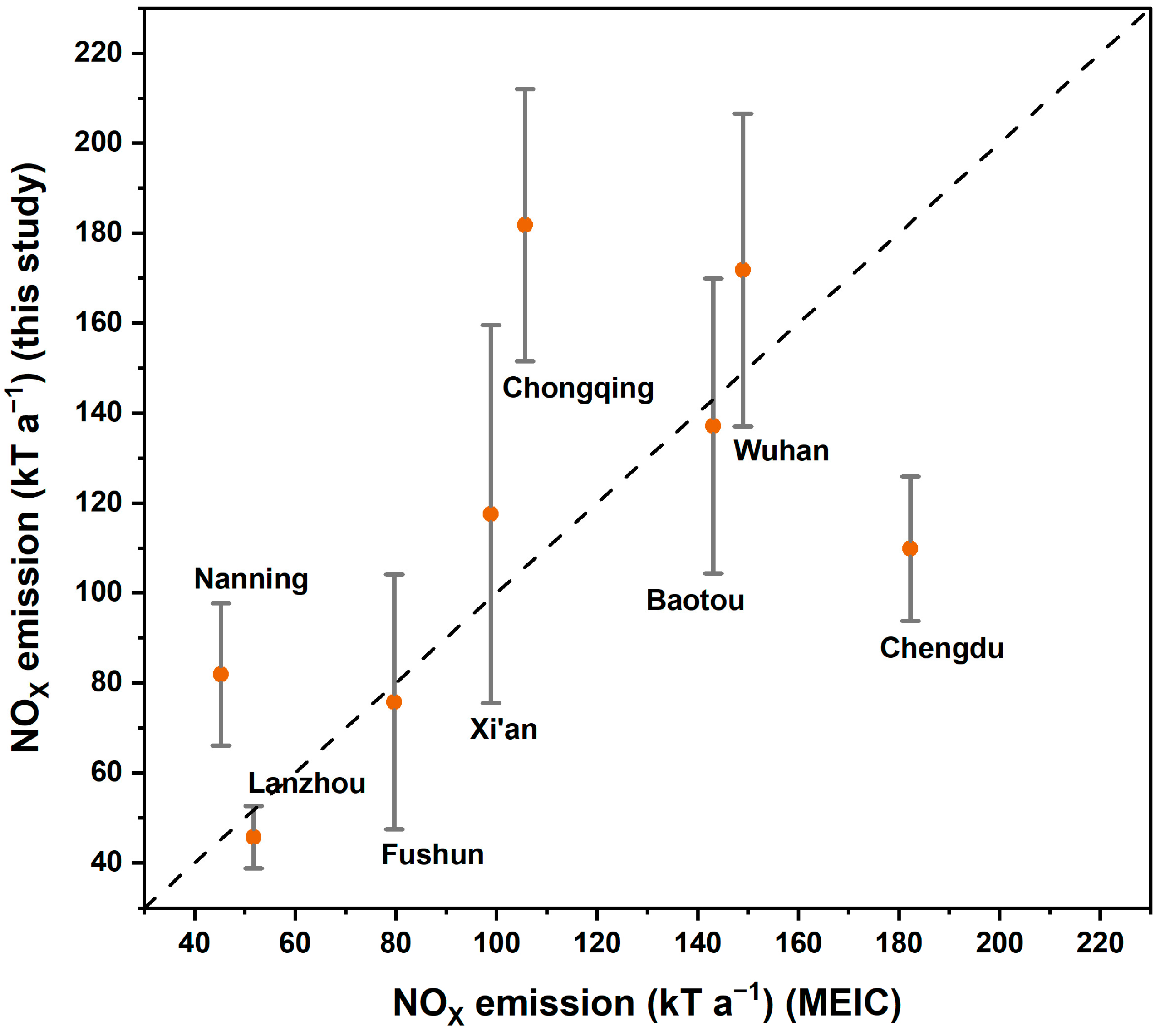
The average NOx emission data estimated for eight cities over five years were also compared with the data reported in the Multi-resolution Emission Inventory for China (MEIC) database for the years 2018 to 2020. Figure 3 presents a comparison between the estimated NOx emissions for these cities and the average values reported in the MEIC database for the same period; the error bars in the figure represent the standard deviation of multiple days’ estimates. It was observed that the majority of NOx emission quantities reported in the MEIC database were lower than those estimated in this study using the EMG method. One possible explanation for this phenomenon is that the EMG method is more sensitive to emissions close to the measurement time, whereas the MEIC database provides an average over all times. Furthermore, a significant discrepancy was noted in the NOx emissions reported for Chengdu and Chongqing in the MEIC inventory compared to the estimates from this study. We attribute this discrepancy primarily to two reasons: firstly, the topography of these cities is predominantly basins and mountainous regions, which can hinder pollutant dispersion compared to other areas, leading to pollutant accumulation; secondly, the presence of numerous mountains in these areas increases cloud fraction, resulting in fewer effective observations by satellites and, consequently, greater estimation uncertainty. Additionally, in Nanning, due to lower emission quantities and less distinct separation from the background concentrations, fewer plumes were observed in satellite imagery, also leading to larger estimation discrepancies.
3.3. Weekend Effect
Human activities peak on weekdays and decrease over weekends, leading to a reduction in urban NOx emissions during weekends [28,29,30,31,32]. This pattern should be reflected in the comparison of NOx emissions between weekdays and weekends. The degree of difference between weekend and weekday emissions depends on the characteristics of different NOx emission sources and regional human activity patterns. To investigate the weekly cycle effect, the estimated results were categorized into weekdays and weekends, with Figure 4 showing the ratio of NOx emissions between weekdays and weekends. We observed that NOx emissions were higher on weekdays than weekends in six cities, particularly in Baotou, where weekend NOx emissions decreased by approximately 60%. Previous research [32,33] indicated an average ratio of weekday-to-weekend NO2 column densities in all major Chinese cities of 0.97 ± 0.02, not demonstrating a significant weekend effect, which is related but not identical to NOx emissions. Additionally, K. Lange et al. [34] observed a weekend-to-weekday ratio of approximately 0.79 in Wuhan, China, which is in good agreement with the findings of our study. In terms of NOx emissions, recent years have seen a more pronounced reduction in weekend emissions in some cities. However, an exception was observed in Chengdu and Lanzhou, where slight increases in weekend emissions were noted, with increases around 20%.
3.4. Seasonal Variation
To investigate the seasonal variations in NOx emissions, we divided the estimated results into four seasons and calculated the average emission rate for each season. Winter spans December to February (DJF), spring from March to May (MAM), summer from June to August (JJA), and autumn from September to November (SON). Due to factors such as ozone limitations and cloud cover, observational conditions vary across seasons, affecting the number of successful estimates per season. We analyzed cities with more than three valid estimates per season, resulting in five of the eight cities being included in the analysis. Figure 5 presents the seasonal average estimates. Among the five cities analyzed in our study, NOx emissions were found to be higher in winter than in summer, notably in Baotou and Wuhan, where winter emissions were more than twice those of summer. In comparison with the inventory, this phenomenon is believed to be associated with the heating sector during winter, not only in cities with centralized heating in the north but also in areas without centralized heating. The use of air conditioning or other heating facilities leads to higher electricity consumption during winter, thereby increasing NOx emissions compared to summer.
We also calculated the emission ratios for summer and winter and the proportions reported by the MEIC inventory, depicted in Figure 6. Our results showed more pronounced seasonal variations compared to the inventory-reported values. Emission inventories are typically calculated based on statistical data and emission factors; for instance, in the transportation sector, inventories estimate emissions by multiplying the number of vehicles at the county level, serving as the activity level, by emission factors assigned according to vehicle types. This approach overlooks the impact of seasonal changes on emission factors, explaining why the inventory reports do not exhibit significant seasonal variations. K. Lange et al. [34] observed notable seasonal variations in Wuhan, China, one of the three cities in all study areas with the lowest winter-to-summer ratios. They reported a summer-to-winter ratio of approximately 0.3 for Wuhan, which aligns with our study’s findings, where the summer-to-winter ratio for Wuhan is estimated at 0.25.
4. Future Research
4.1. Estimation in the Polluted Background
A significant limitation of the EMG method is its potential ineffectiveness within polluted scenarios, where emission sources often represent emission hotspots. Therefore, exploring improvement measures to estimate emission strengths from sources within high-pollution backgrounds is necessary. This requires the precise identification and separation of pollution background concentrations, which can be achieved by collecting data during periods devoid of major emission source activities (such as nighttime or specific seasons) or by defining different sectors to analyze wind direction and pollution dispersion. This approach aids in identifying and isolating emission sources from specific directions, reducing interference from surrounding pollution backgrounds. Implementing these strategies will enhance the applicability of the EMG method in polluted environments, enabling accurate estimation of emission strengths from critical sources within high-pollution backgrounds.
4.2. More Real-Time Monitoring
This study utilizes observations from instruments mounted on Sentinel-5, a sun-synchronous orbit satellite that provides near-global coverage data once daily. The limitation of satellite measurement timing, using measurements from a single moment within the day to represent the average daily emission strength, can lead to biases. Therefore, observational data with higher temporal resolution are required to more accurately characterize the emission patterns of NOx from sources, offering more detailed emission information. Subsequent launches of geosynchronous satellites equipped with sensors, such as GEMS, TEMPO, and Sentinel-4, are capable of providing multiple sets of observational data for targeted regions within a day. This significantly enhances the timeliness of obtaining emission information from source areas, providing new perspectives for the timely monitoring and intervention of atmospheric pollution processes.
5. Conclusions
This investigation, for the first time, quantified urban daily NOx emissions by leveraging real plume observations captured during singular overpasses by the TROPOMI. It substantiates the efficacy of the EMG methodology in estimating emissions from genuine plumes and elucidates the methodological applicability of EMG. Moreover, it delves into the temporal dynamics of urban NOx emissions, articulating both weekend and seasonal variations. The observed phenomena of diminished emissions during weekends and escalated emissions during the winter season (or heating period) across the majority of the cities examined furnish novel avenues for the refinement of urban NOx emission estimation and monitoring, thereby contributing to the strategic mitigation of atmospheric pollution challenges.
Author Contributions
Conceptualization, T.T. and L.Z.; data curation, T.T. and D.F.; formal analysis, T.T., H.Z., X.Y., D.F., X.L. and H.T.; funding acquisition, L.Z.; investigation, T.T. and X.Y.; methodology, T.T.; supervision, L.Z., H.Z., X.Y., D.F., X.L., H.T. and S.L.; validation, T.T.; writing—original draft, T.T.; writing—review and editing, T.T., L.Z., H.Z., X.L., H.T. and S.L. All authors have read and agreed to the published version of the manuscript.
Funding
This study was supported by the National Key Research and Development Program of China (Grant No. 2023YFB3907405) and a grant from the State Key Laboratory of Resources and Environmental Information System, Chinese Academy of Sciences.
Institutional Review Board Statement
Not applicable.
Informed Consent Statement
Not applicable.
Data Availability Statement
TROPOMI data from July 2018 onwards are freely available at https://browser.dataspace.copernicus.eu/ (accessed on 19 April 2024). The Meteorological data from the ERA5 reanalysis are freely available from the Copernicus Climate Change (C3S) climate data store (CDS) at https://cds.climate.copernicus.eu/#!/home (accessed on 19 April 2024). The MEIC emission inventory (v1.4) from 1990 to 2020 are freely available at http://meicmodel.org.cn (accessed on 19 April 2024).
Acknowledgments
Appreciation is extended to the anonymous reviewers for their careful review and constructive suggestions to improve the manuscript.
Conflicts of Interest
The authors declare no conflicts of interest.
References
- Solomon, S. Stratospheric ozone depletion: A review of concepts and history. Rev. Geophys. 1999, 37, 275–316. [Google Scholar] [CrossRef]
- Seinfeld, J.H. Clouds, contrails and climate. Nature 1998, 391, 837–838. [Google Scholar] [CrossRef]
- Shindell, D.T.; Faluvegi, G.; Koch, D.M.; Schmidt, G.A.; Unger, N.; Bauer, S.E. Improved attribution of climate forcing to emissions. Science 2009, 326, 716–718. [Google Scholar] [CrossRef]
- Seinfeld, J.H.; Pandis, S.N. Atmospheric Chemistry and Physics: From Air Pollution to Climate Change; John Wiley & Sons: Hoboken, NJ, USA, 2016. [Google Scholar]
- Sillman, S.; Logan, J.A.; Wofsy, S.C. The sensitivity of ozone to nitrogen oxides and hydrocarbons in regional ozone episodes. J. Geophys. Res. Atmos. 1990, 95, 1837–1851. [Google Scholar] [CrossRef]
- Butler, T.; Lawrence, M.; Gurjar, B.R.; Van Aardenne, J.; Schultz, M.; Lelieveld, J. The representation of emissions from megacities in global emission inventories. Atmos. Environ. 2008, 42, 703–719. [Google Scholar] [CrossRef]
- Zhao, Y.; Nielsen, C.P.; Lei, Y.; McElroy, M.B.; Hao, J. Quantifying the uncertainties of a bottom-up emission inventory of anthropogenic atmospheric pollutants in China. Atmos. Chem. Phys. 2011, 11, 2295–2308. [Google Scholar] [CrossRef]
- Beirle, S.; Boersma, K.F.; Platt, U.; Lawrence, M.G.; Wagner, T. Megacity emissions and lifetimes of nitrogen oxides probed from space. Science 2011, 333, 1737–1739. [Google Scholar] [CrossRef]
- de Foy, B.; Wilkins, J.L.; Lu, Z.; Streets, D.G.; Duncan, B.N. Model evaluation of methods for estimating surface emissions and chemical lifetimes from satellite data. Atmos. Environ. 2014, 98, 66–77. [Google Scholar] [CrossRef]
- Liu, F.; Beirle, S.; Zhang, Q.; Dörner, S.; He, K.; Wagner, T. NOx lifetimes and emissions of cities and power plants in polluted background estimated by satellite observations. Atmos. Chem. Phys. 2016, 16, 5283–5298. [Google Scholar] [CrossRef]
- Liu, F.; Tao, Z.; Beirle, S.; Joiner, J.; Yoshida, Y.; Smith, S.J.; Knowland, K.E.; Wagner, T. A new method for inferring city emissions and lifetimes of nitrogen oxides from high-resolution nitrogen dioxide observations: A model study. Atmos. Chem. Phys. 2022, 22, 1333–1349. [Google Scholar] [CrossRef]
- Fioletov, V.E.; McLinden, C.; Krotkov, N.; Li, C. Lifetimes and emissions of SO2 from point sources estimated from OMI. Geophys. Res. Lett. 2015, 42, 1969–1976. [Google Scholar] [CrossRef]
- Dammers, E.; McLinden, C.A.; Griffin, D.; Shephard, M.W.; Van Der Graaf, S.; Lutsch, E.; Schaap, M.; Gainairu-Matz, Y.; Fioletov, V.; Van Damme, M. NH3 emissions from large point sources derived from CrIS and IASI satellite observations. Atmos. Chem. Phys. 2019, 19, 12261–12293. [Google Scholar] [CrossRef]
- Ganbat, G.; Lee, H.; Jo, H.-W.; Jadamba, B.; Karthe, D. Assessment of COVID-19 Impacts on Air Quality in Ulaanbaatar, Mongolia, Based on Terrestrial and Sentinel-5P TROPOMI Data. Aerosol Air Qual. Res. 2022, 22, 220196. [Google Scholar] [CrossRef]
- Naeem, W.; Kim, J.; Lee, Y.G. Spatiotemporal variations in the air pollutant NO2 in some regions of Pakistan, India, China, and Korea, before and after COVID-19, based on ozone monitoring instrument data. Atmosphere 2022, 13, 986. [Google Scholar] [CrossRef]
- Schiavo, B.; Morton-Bermea, O.; Arredondo-Palacios, T.E.; Meza-Figueroa, D.; Robles-Morua, A.; García-Martínez, R.; Valera-Fernández, D.; Inguaggiato, C.; Gonzalez-Grijalva, B. Analysis of COVID-19 Lockdown Effects on Urban Air Quality: A Case Study of Monterrey, Mexico. Sustainability 2022, 15, 642. [Google Scholar] [CrossRef]
- Griffin, D.; McLinden, C.A.; Dammers, E.; Adams, C.; Stockwell, C.; Warneke, C.; Bourgeois, I.; Peischl, J.; Ryerson, T.B.; Zarzana, K.J. Biomass burning nitrogen dioxide emissions derived from space with TROPOMI: Methodology and validation. Atmos. Meas. Tech. Discuss. 2021, 2021, 7929–7957. [Google Scholar] [CrossRef]
- Veefkind, J.P.; Aben, I.; McMullan, K.; Förster, H.; De Vries, J.; Otter, G.; Claas, J.; Eskes, H.; De Haan, J.; Kleipool, Q. TROPOMI on the ESA Sentinel-5 Precursor: A GMES mission for global observations of the atmospheric composition for climate, air quality and ozone layer applications. Remote Sens. Environ. 2012, 120, 70–83. [Google Scholar] [CrossRef]
- Hu, H.; Landgraf, J.; Detmers, R.; Borsdorff, T.; Aan de Brugh, J.; Aben, I.; Butz, A.; Hasekamp, O. Toward global mapping of methane with TROPOMI: First results and intersatellite comparison to GOSAT. Geophys. Res. Lett. 2018, 45, 3682–3689. [Google Scholar] [CrossRef]
- Lin, J.-S.; Hildemann, L.M. Analytical solutions of the atmospheric diffusion equation with multiple sources and height-dependent wind speed and eddy diffusivities. Atmos. Environ. 1996, 30, 239–254. [Google Scholar] [CrossRef]
- Tian, Y.; Liu, C.; Sun, Y.; Borsdorff, T.; Landgraf, J.; Lu, X.; Palm, M.; Notholt, J. Satellite observations reveal a large CO emission discrepancy from industrial point sources over China. Geophys. Res. Lett. 2022, 49, e2021GL097312. [Google Scholar] [CrossRef]
- Li, M.; Liu, H.; Geng, G.; Hong, C.; Liu, F.; Song, Y.; Tong, D.; Zheng, B.; Cui, H.; Man, H. Anthropogenic emission inventories in China: A review. Natl. Sci. Rev. 2017, 4, 834–866. [Google Scholar] [CrossRef]
- Zheng, B.; Tong, D.; Li, M.; Liu, F.; Hong, C.; Geng, G.; Li, H.; Li, X.; Peng, L.; Qi, J. Trends in China’s anthropogenic emissions since 2010 as the consequence of clean air actions. Atmos. Chem. Phys. 2018, 18, 14095–14111. [Google Scholar] [CrossRef]
- Fioletov, V.; McLinden, C.; Krotkov, N.; Moran, M.; Yang, K. Estimation of SO2 emissions using OMI retrievals. Geophys. Res. Lett. 2011, 38, L21811. [Google Scholar] [CrossRef]
- McLinden, C.A.; Fioletov, V.; Shephard, M.W.; Krotkov, N.; Li, C.; Martin, R.V.; Moran, M.D.; Joiner, J. Space-based detection of missing sulfur dioxide sources of global air pollution. Nat. Geosci. 2016, 9, 496–500. [Google Scholar] [CrossRef]
- Xu, T.; Zhang, C.; Xue, J.; Hu, Q.; Xing, C.; Liu, C. Estimating Hourly Nitrogen Oxide Emissions over East Asia from Geostationary Satellite Measurements. Environ. Sci. Technol. Lett. 2023, 11, 122–129. [Google Scholar] [CrossRef]
- Beirle, S.; Borger, C.; Dörner, S.; Eskes, H.; Kumar, V.; de Laat, A.; Wagner, T. Catalog of NOx emissions from point sources as derived from the divergence of the NO2 flux for TROPOMI. Earth Syst. Sci. Data Discuss. 2021, 2021, 2995–3012. [Google Scholar] [CrossRef]
- Goldberg, D.L.; Lu, Z.; Streets, D.G.; de Foy, B.; Griffin, D.; McLinden, C.A.; Lamsal, L.N.; Krotkov, N.A.; Eskes, H. Enhanced capabilities of TROPOMI NO2: Estimating NOx from north american cities and power plants. Environ. Sci. Technol. 2019, 53, 12594–12601. [Google Scholar] [CrossRef]
- Lorente, A.; Boersma, K.; Eskes, H.; Veefkind, J.; Van Geffen, J.; De Zeeuw, M.; Denier Van Der Gon, H.; Beirle, S.; Krol, M. Quantification of nitrogen oxides emissions from build-up of pollution over Paris with TROPOMI. Sci. Rep. 2019, 9, 20033. [Google Scholar] [CrossRef]
- Goldberg, D.L.; Anenberg, S.C.; Kerr, G.H.; Mohegh, A.; Lu, Z.; Streets, D.G. TROPOMI NO2 in the United States: A detailed look at the annual averages, weekly cycles, effects of temperature, and correlation with surface NO2 concentrations. Earth’s Future 2021, 9, e2020EF001665. [Google Scholar] [CrossRef]
- Crippa, M.; Solazzo, E.; Huang, G.; Guizzardi, D.; Koffi, E.; Muntean, M.; Schieberle, C.; Friedrich, R.; Janssens-Maenhout, G. High resolution temporal profiles in the Emissions Database for Global Atmospheric Research. Sci. Data 2020, 7, 121. [Google Scholar] [CrossRef]
- Beirle, S.; Platt, U.; Wenig, M.; Wagner, T. Weekly cycle of NO2 by GOME measurements: A signature of anthropogenic sources. Atmos. Chem. Phys. 2003, 3, 2225–2232. [Google Scholar] [CrossRef]
- Stavrakou, T.; Müller, J.-F.; Bauwens, M.; Boersma, K.; Van Geffen, J. Satellite evidence for changes in the NO2 weekly cycle over large cities. Sci. Rep. 2020, 10, 10066. [Google Scholar] [CrossRef] [PubMed]
- Lange, K.; Richter, A.; Burrows, J.P. Variability of nitrogen oxide emission fluxes and lifetimes estimated from Sentinel-5P TROPOMI observations. Atmos. Chem. Phys. 2022, 22, 2745–2767. [Google Scholar] [CrossRef]
Figure 1.
Mean tropospheric vertical column NO2 concentrations and study cities (2018–2022) (labeled by red circles).
Figure 1.
Mean tropospheric vertical column NO2 concentrations and study cities (2018–2022) (labeled by red circles).

Figure 2.
Satellite data and fitting results (Wuhan city on 1 April 2023 as an example). (a) Real plume dispersion observed by TROPOMI over Wuhan city, with red arrows showing the wind direction; (b) satellite observation data and model fitting results.
Figure 2.
Satellite data and fitting results (Wuhan city on 1 April 2023 as an example). (a) Real plume dispersion observed by TROPOMI over Wuhan city, with red arrows showing the wind direction; (b) satellite observation data and model fitting results.

Figure 3.
NOx emissions derived from 5-year TROPOMI data for eight cities using the EMG method are compared with NOx emissions reported from the MEIC emissions database. The dashed line indicates a 1:1 ratio. The error bars are the standard deviation of the emission results derived by the EMG fitting procedure.

Figure 4.
Ratio of NOx emissions on weekday to weekend. The bar graphs show the average emission rates on weekdays and weekends, and the dotted line graphs show the ratio between them.
Figure 4.
Ratio of NOx emissions on weekday to weekend. The bar graphs show the average emission rates on weekdays and weekends, and the dotted line graphs show the ratio between them.

Figure 5.
Average emission rate of NOx in four seasons.

Figure 6.
Summer-to-winter ratio for this study and MEIC inventory.


Table 1.
Latitude and longitude of the study city centers.
| Study Cities | Latitude (Degree) | Longitude (Degree) |
|---|---|---|
| Baotou | 40.38 | 109.59 |
| Wuhan | 30.57 | 114.28 |
| Xi’an | 34.24 | 108.91 |
| Chengdu | 30.63 | 104.12 |
| Chongqing | 29.58 | 106.51 |
| Lanzhou | 36.08 | 103.75 |
| Nanning | 22.81 | 108.30 |
| Fushun | 41.85 | 123.93 |
Disclaimer/Publisher’s Note: The statements, opinions and data contained in all publications are solely those of the individual author(s) and contributor(s) and not of MDPI and/or the editor(s). MDPI and/or the editor(s) disclaim responsibility for any injury to people or property resulting from any ideas, methods, instructions or products referred to in the content. |
© 2024 by the authors. Licensee MDPI, Basel, Switzerland. This article is an open access article distributed under the terms and conditions of the Creative Commons Attribution (CC BY) license (https://creativecommons.org/licenses/by/4.0/).
Share and Cite
MDPI and ACS Style
Tang, T.; Zhang, L.; Zhu, H.; Ye, X.; Fan, D.; Li, X.; Tong, H.; Li, S. Quantifying Urban Daily Nitrogen Oxide Emissions from Satellite Observations. Atmosphere 2024, 15, 508. https://doi.org/10.3390/atmos15040508
AMA Style
Tang T, Zhang L, Zhu H, Ye X, Fan D, Li X, Tong H, Li S. Quantifying Urban Daily Nitrogen Oxide Emissions from Satellite Observations. Atmosphere. 2024; 15(4):508. https://doi.org/10.3390/atmos15040508
Chicago/Turabian StyleTang, Tao, Lili Zhang, Hao Zhu, Xiaotong Ye, Donghao Fan, Xingyu Li, Haoran Tong, and Shenshen Li. 2024. "Quantifying Urban Daily Nitrogen Oxide Emissions from Satellite Observations" Atmosphere 15, no. 4: 508. https://doi.org/10.3390/atmos15040508
Note that from the first issue of 2016, this journal uses article numbers instead of page numbers. See further details here.