
Machine Learning Forecast of Dust Storm Frequency in Saudi Arabia Using Multiple Features


1
Information Systems Department, College of Computer and Information Sciences, King Saud University, P.O. Box. 145111, Riyadh 11362, Saudi Arabia
2
Space Technologies Institute, King Abdulaziz City for Science and Technology, P.O. Box 6086, Riyadh 11442, Saudi Arabia
*
Author to whom correspondence should be addressed.
Atmosphere 2024, 15(5), 520; https://doi.org/10.3390/atmos15050520
Submission received: 10 March 2024
/
Revised: 18 April 2024
/
Accepted: 20 April 2024
/
Published: 24 April 2024
(This article belongs to the Special Issue New Insights in Air Quality Assessment: Forecasting and Monitoring)
Abstract
:Dust storms are significant atmospheric events that impact air quality, public health, and visibility, especially in arid Saudi Arabia. This study aimed to develop dust storm frequency predictions for Riyadh, Jeddah, and Dammam by integrating meteorological and environmental variables. Our models include multiple linear regression, support vector machine, gradient boosting regression tree, long short-term memory (LSTM), and temporal convolutional network (TCN). This study highlights the effectiveness of LSTM and TCN models in capturing the complex temporal dynamics of dust storms and demonstrates that they outperform traditional methods, as evidenced by their lower mean absolute error (MAE) and root mean square error (RMSE) values and higher R2 score. In Riyadh, the TCN model demonstrates its remarkable performance, with an R2 score of 0.51, an MAE of 2.80, and an RMSE of 3.48, highlighting its precision, adaptability, and responsiveness to changes in dust storm frequency. Conversely, in Dammam, the LSTM model proved to be the most accurate, achieving an MAE of 3.02, RMSE of 3.64, and R2 score of 0.64. In Jeddah, the LSTM model also exhibited an MAE of 2.48 and an RMSE of 2.96. This research shows the potential of using deep learning models to improve the accuracy and reliability of dust storm frequency forecasts.
1. Introduction
Dust storms are meteorological phenomena characterized by strong winds that lift large quantities of dust into the atmosphere, thereby presenting considerable environmental, economic, and health challenges [1]. The Middle East, with its characteristic arid and semi-arid climates, is a major source of dust emissions due to significant influences of deserts (e.g., the Arabian, Syrian, and Sahara deserts), which are primary sources of particulates [2]. Wind patterns, such as the Shamal winds in the Arabian Peninsula, and seasonal variations influence dust storms, which can travel thousands of kilometers before deposition [3]. Saudi Arabia, with its vast deserts and distinctive topography, is particularly susceptible to dust storms, especially those arising from local dust sources [4,5,6]. Although dust storms occur throughout the entire year in Saudi Arabia, the frequency and intensity of these storms vary regionally based on the season [7]. This variability significantly affects visibility and air quality, leading to an urgent need for accurate prediction models to facilitate effective mitigation and early warning systems [8].
The detection and monitoring of dust storms rely heavily on ground-based observations and satellite remote sensing technologies [9]. Weather stations with visibility sensors and particulate matter (PM) monitors provide immediate data that are vital for early warning systems; for example, low-cost sensors offer unconventional data for air quality analysis [10]. The World Meteorological Organization (WMO) uses a specialized coding system to categorize weather phenomena [11], and the present study adopted the WMO code for defining dust storms.
Traditional methods for forecasting the frequency of dust storms have primarily focused on the observation and statistical analysis of current and historical weather to identify patterns and trends [7,12], along with the utilization of numerical weather prediction through climate models to simulate atmospheric conditions [9]. However, the complex and dynamic factors that influence dust storms, such as dust sources, vegetation cover, and land use changes, require a more sophisticated and integrated approach than these methods presently provide [13].
Recent advancements in dust storm forecasting have incorporated machine learning [14]. For instance, some studies have used machine learning models, such as support vector machine (SVM), naive Bayesian, random forest, and k-nearest neighbors models, for short-term forecasting as daily predictions across various regions, including the Middle East, with significant contributions from studies by Ali et al. [15], Al Murayziq et al. [16], and Shaiba et al. [17]. For monthly forecasts, Aryal [18,19] explored the prediction of fine and coarse dust using multiple linear regression (MLR) and SVM. Zhang et al. [20] also focused on frequency prediction by balancing the data under the assumption that dust storm occurrence is a rare class. They then applied AdaBoost with a random forest model and trained it with meteorological data to forecast the classification of the frequency category from 0 to 9 classes.
Beyond meteorological data, the role of land cover and vegetation in dust storm dynamics is critical. Ebrahimi-Khusfi et al. [21] applied machine learning models to predict the number of dusty days around wetlands. Their work highlights the effectiveness of stochastic gradient boosting (SGB) in forecasting dusty days while adding land cover areas. They then measured feature contributions using game theory. Another study by Ebrahimi-Khusfi et al. [22] also used meteorological data with wetland-dried areas as input features and then compared SVM, conditional inference random forest (CRF), and SGB. The SGB model, in conjunction with various feature selection techniques, showed the highest accuracy. Nabavi et al. [23] examined the relationship between dust emission and the normalized difference vegetation index (NDVI), among other variables, to predict the monthly dust aerosol index. However, the current forecasting methods have limitations, which are now being addressed using deep learning techniques that specialize in temporal data processing [14]. Deep learning models, such as long short-term memory (LSTM) networks and temporal convolutional networks (TCN), have shown great promise in environmental modeling, particularly because of their ability to capture complex temporal relationships in data. These models, which are adept at handling sequences and time series, can offer further understanding and prediction of evolving phenomena, such as dust storms [24].
Previous studies have used different machine learning models to predict dust storms using various data, such as temperature, humidity, pressure, and wind speed. However, the occurrence of dust storms is also heavily influenced by environmental factors and dust sources that have not yet been addressed [5,6,25]. Also, explorations of dust storm frequency as a time series are lacking. Utilizing LSTM and TCN with sliding window techniques could address this gap, thereby improving dust storm prediction accuracy by incorporating these temporal dynamics. Accordingly, the aims of the present study were: (1) to select the optimal combination of input data for predicting the monthly frequency of dust storms using feature selection techniques; (2) to assess the efficacy of multiple machine learning and deep learning models, including multiple linear regression (MLR), support vector regression (SVR), and gradient boosting regression tree (GBRT), along with deep learning models (e.g., LSTM and TCN), in forecasting these phenomena; and (3) to use Shapley additive explanations (SHAP) values to investigate the influence of climate and environmental variables, such as meteorological data, NDVI, land use, and identified dust sources, on the predictive models’ performance. We also employed root-mean-square error (RMSE), mean absolute error (MAE), and coefficient of determination (R2) metrics to evaluate the model’s accuracy. This approach enabled a comparison of prediction outcomes across various cities, highlighting the impact of different factors influencing dust storms.
2. Data and Methods
2.1. Study Area
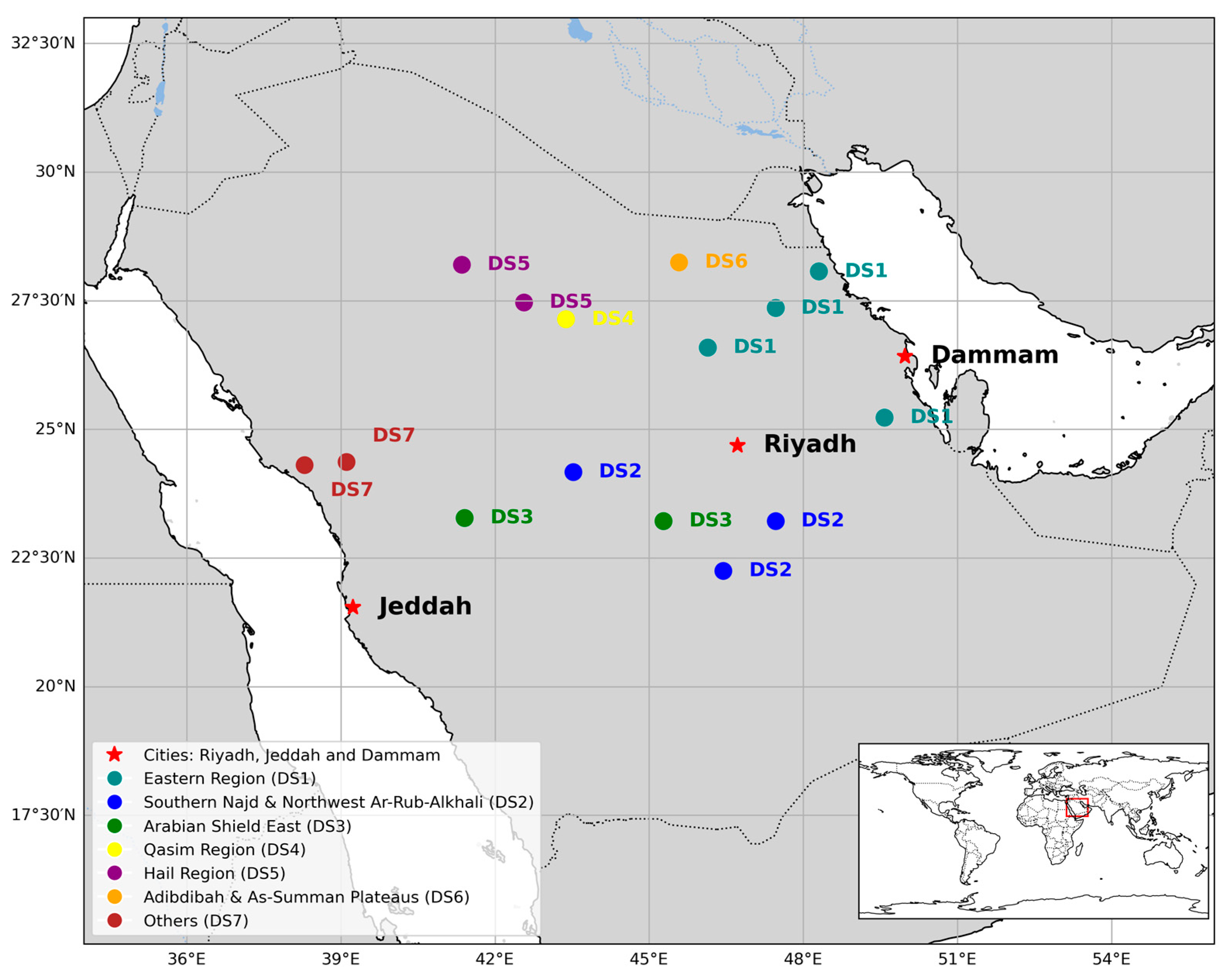
Saudi Arabia experiences some of the most intense and frequent dust storms globally. Vast arid expanses, varied topography, and seasonal climatic extremes characterize its distinctive geography. Three cities, including Riyadh, Jeddah, and Dammam, were selected for comparison based on their significant geographical and demographic importance within the country (Figure 1). Riyadh, located at 24.7136° N and 46.6753° E, is the capital city in the central region. Jeddah, located at 21.4858° N and 39.1925° E, is situated on the western coast overlooking the Red Sea, while Dammam, located at 26.4207° N and 50.0888° E, is in the eastern region near the Arabian Gulf. These cities are strategically located on the Arabian Peninsula and are surrounded by expansive deserts, including the vast Rub’ al Khali. The arid nature and prevailing winds significantly influence dust storm generation.
In this study, we considered local dust sources in Saudi Arabia that directly impact the cities of Riyadh, Jeddah, and Dammam. Identifying these dust sources was informed by a previous study that employed the analysis of various satellite images and backward trajectories to identify the dust source regions associated with the dustiest days experienced in Riyadh, Jeddah, and Dammam over the 2000–2005 period [6]. In total, 45 dust-source areas were identified, distributed across local source regions within Saudi Arabia and external regions. The selected local dust source regions included the Eastern Region (DS1), the Southern Najd and Northwest Ar-Rub-Alkhali Region (DS2), the Eastern Region of the Arabian Shield (DS3), the Qasim Region (DS4), the Hail Region (DS5), the Adibdibah and As-Summan Plateau Region (DS6), and Others (DS7) (Figure 1).
2.2. Data Collection
This study considered the climate and environmental variables that predict the next month’s dust storm days. The following data were collected for 16 years, from 2005 to 2020, from different data sources:
- Dust storm frequency
The dust storm frequency data were obtained from the Saudi National Centre for Meteorology. This dataset consists of daily records, with weather codes representing different weather conditions. In this study, dust storm occurrence was defined by weather codes (06, 07, 08, 09, and 30 to 35) as defined by the World Meteorological Organization (WMO) [11].
- Meteorological Data
The meteorological data for Riyadh, Jeddah, and Dammam included temperature, relative humidity, pressure, vapor pressure, wind speed, wind direction, and precipitation. These were daily measurements obtained from the Saudi National Center for Meteorology. Additionally, the meteorological data for local dust sources, obtained from the POWER/MERRA-2 dataset, were used as daily measurements [26].
- Environmental Data
- ○
- The land cover data included classes for barren land, water bodies, urban and built-up areas, and vegetation-related classes. They were sourced from MODIS products and have spatial resolutions of 500 m. The Google Earth Engine was used to calculate the mean for each year of the study period [27].
- ○
- Another variable used to identify vegetation cover was the NDVI. This dataset, acquired from the MODIS satellite, has a spatial resolution of 1 km and a temporal resolution of every 16 days. The Google Earth Engine was used to calculate the mean [28].
This study considered climate and environmental variables; the data sources and resolutions used are shown in Table 1.
2.3. Data Preprocessing
In the data preprocessing stage, several steps were undertaken to ensure the quality and consistency of the dataset. The following procedures were implemented:
- Handling missing variables: Missing values in the meteorological daily dataset were replaced with the mean value of the respective variable. This included one missing value in wind speed and wind prevailing direction.
- We addressed potential inconsistencies and errors in some variables within the dataset by adjusting outliers to within valid ranges and correcting abnormally high values with the mean.
- Wind direction: The continuous wind direction data were discretized into eight cardinal directions (north, northeast, east, southeast, south, southwest, west, and northwest) to facilitate model interpretation and accommodate categorical inputs. One-hot encoding was then used to represent each direction as a binary vector. This encoding enabled the model to capture directional patterns without assumptions about the numerical relationships among the directions.
- Preparing the dataset as monthly data: We calculated the monthly dust storm frequency for 2005–2020 by summing up the number of dust storm days per month. We computed the monthly mean for other predictors, such as temperature, humidity, and wind speed, to capture the overall trend. To further explore the relationship between wind patterns and dusty days, we augmented the dataset with two additional columns: (1) the sum of days in each month with the wind speed exceeding 20 km/h, and (2) the sum of days with the wind speed exceeding 20 km/h across all dust sources within each group. These additions expose the potential influence of high-wind events on dust storm occurrences [22].
- Incorporating seasonality: We explicitly accounted for potential seasonal influences on dust storm patterns by creating a new numerical variable to represent the season for each data point (spring = 1, summer = 2, autumn = 3, and winter = 4).
- Historical dust storm frequency: Dust storm occurrences often exhibit temporal patterns, meaning that events in one month can be correlated with those in the following months. To capture this, we incorporated the month’s dust storm frequency as a feature.
2.4. Normalization
For our study, min–max normalization was applied to all numerical features. This normalization technique adjusted each feature’s values to a consistent range between 0.05 and 0.95, according to the formula:
where xn is the normalized value of a specific feature, xo denotes the original value, and xmin and xmax represent the minimum and maximum values, respectively, of a specific feature within the entire dataset. The range from 0.05 to 0.95 was selected to circumvent potential saturation issues at the data’s extremes, thereby ensuring an adequate spread for effective model training. This normalization approach closely follows the approach outlined in [22]. The resulting normalized dataset comprised 192 monthly observations for each city.
2.5. Feature Selection
Our approach taken for feature selection initially addressed the issue of multicollinearity among the independent variables, as strong correlations can lead to unreliable estimates and predictions [29]. Employing the Pearson correlation coefficient as a standard measure for assessing linear associations [30,31], we identified and excluded highly correlated features (above a 0.8 threshold) from our dataset across Riyadh, Jeddah, and Dammam [29,32].
We then utilized the random forest algorithm, based on its robustness in handling complex data interactions, to evaluate the relative importance of features within each correlated pair. This algorithm enabled the identification and exclusion of the less important feature from each highly correlated pair, thereby ensuring that the final feature set was independent and impactful. It also reduced redundancy, which improved the model performance [33].
2.6. Machine Learning Methods
In this study, the following five predictive models were applied:
2.6.1. Multilinear Regression (MLR)
MLR is widely used in prediction time series analyses in the atmospheric field [34,35] and for dust aerosol and air quality predictions that consider multiple features [23,36]. This method offers low computational demands for exploring relationships between one dependent variable and one or more independent variables by fitting the linear equation of the observed data. This study constructed an MLR model using next month’s dust storm frequency (y) as the dependent variable and relevant climate and environmental factors (x1, …, xn) as independent variables. The MLR equation is as follows:
where y is the dependent variable, a and b1, …, bn: are regression coefficients for each independent variable, x1, …, xn are independent climate and environmental variables, and ε is the error term [37].
y = a + b1x1 + b2x2 + …+ bnxn + ε
2.6.2. Support Vector Regression (SVR)
SVR is employed for its structural risk minimization principle [38]. This principle enables the capture of non-linear relationships and has been utilized in time series forecasting and dust events [34,39]. The SVR equation is given by:
where k(z) represents the SVR prediction function for the input data z = (z1, z2, …, zn), v is the weight factor, c is the constant term, and φ(z) is the kernel function that transforms the input into a higher-dimensional feature space.
y = k(z) = vφ(z) + c
2.6.3. Gradient Boosting Regression Tree (GBRT)
GBRT is a machine learning algorithm for regression tasks. GBRT combines decision trees and boosting to create an ensemble model that delivers accurate predictions [40]. It iteratively builds multiple weak regression trees and uses gradient descent to minimize the loss function. The equation represents the GBRT model:
where y represents the predicted value, Σᵢ denotes the summation over individual regression trees, and fᵢ(x) represents the output of each tree.
y = Σᵢ fᵢ(x)
2.6.4. Long Short-Term Memory (LSTM)
As an advanced recurrent neural network (RNN) architecture, LSTM can model long-term dependencies by utilizing gates that regulate information flow, including three distinct gates: the forget gate (ft), the input gate (it), and the output gate (ot) (Figure 2) [41]. These gates control the flow of information, thereby enabling LSTMs to retain or discard information over extended time intervals and to handle the challenges of vanishing and exploding gradients in RNNs, making them effective in learning complex temporal patterns.
LSTM cells feature a dual-output mechanism comprising a cell state and a hidden state. The cell state serves as the long-term memory, whereas the hidden state acts as the short-term memory, capturing information from the most recent input. These states are updated at every time step through gating mechanisms, which depend on the current input (xt), the previous hidden state (ht−1), and the previous cell state (Ct−1).
2.6.5. Temporal Convolutional Networks (TCN)
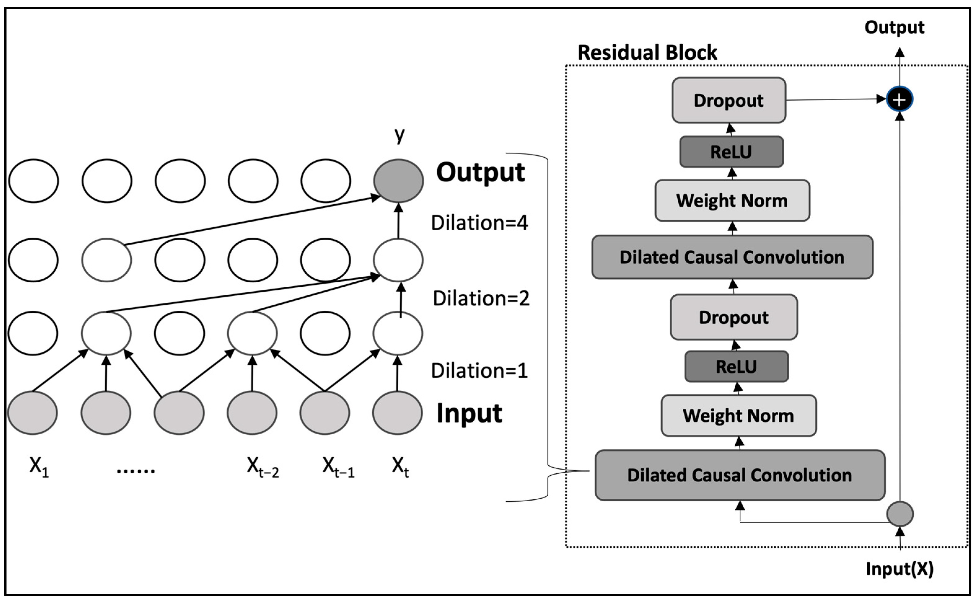
Temporal convolutional networks (TCN) are a type of convolutional neural network (CNN) designed for modeling sequential data (Figure 3) [42]. Unlike the conventional processing approach of CNN and RNN models, which process data sequentially, TCNs utilize time-dilated convolutions, enabling them to capture long-range dependencies with lower computational costs and higher parallelization capabilities and have shown promising results in sequence modeling tasks [43]. Dilated causal convolutions ensure that the model’s predictions rely solely on current and past inputs, making TCNs particularly effective for forecasting tasks. Furthermore, including residual blocks significantly increases the model’s capacity to manage sequences of varying lengths.
2.6.6. Experimental Setup
In this study, our approach utilizes a range of models spanning traditional machine learning and advanced deep learning techniques. The models under consideration are MLR, SVR, GBRT, LSTM, and TCN.
These models (MLR, GBRT, and SVR) were applied using the Scikit-learn library [44]. MLR, a simpler model, was employed in its standard form without hyperparameter tuning. SVR and GBRT were optimized using a grid search for hyperparameter tuning. The hyperparameters for GBRT were chosen based on recommendations [45]. The hyperparameters of the grid search conducted for SVR and GBRT are shown in Table 2.
In the LSTM layer, we utilized the hyperbolic tangent function (tanh) due to its effectiveness in managing the gradient flow over long sequences, as this is crucial for capturing the temporal dynamics inherent in dust storm frequency data. For the dense layers following the LSTM or within the TCN model, the rectified linear unit (ReLU) activation function was applied. ReLU was chosen for its ability to facilitate fast convergence and mitigate the vanishing gradient problem, thus enhancing model efficiency [46]. The adaptive moment estimation (ADAM) optimizer was employed across all deep learning models for its robustness and adaptive learning rate capabilities.
We determined the optimal configuration of our models by conducting a comprehensive grid search and exploring a range of hyperparameters, including the number of processing nodes, epochs, batch sizes, and the number of layers for both LSTM and TCN models, as detailed in Table 3.
By incorporating a grid search, we investigated the impact of different sliding window sizes on the model’s ability to forecast dust storm frequency accurately. We analyzed sequences from the past 1 to 20 months as distinct scenarios to identify the temporal window that best enhances prediction accuracy. For instance, a window size of 3 months entailed aggregating observations from t−2 to t as the input set for predicting the dust storm frequency for the following month, t+1. This was applied to evaluate how different lengths of historical data affected the model’s capacity to recognize temporal patterns, specifically since we had dust source data.
The optimal hyperparameters identified for the LSTM model included a window size of 5 months, 200 nodes, 24 epochs, and a batch size 32.
The TCN model’s optimal settings were a window size of 5 months, three layers with kernel sizes of 5, and dilation rates of 1, 2, 4, and 8, reflecting the model’s capacity to capture both short-term and long-term dependencies in the data. The structure of the LSTM and TCN models and their optimal hyperparameters are detailed in Table 4.
We implemented the persistence method to provide a benchmark for our models’ predictive performances [34]. This forecasting approach assumes that conditions remain constant; that is, it predicts the frequency of dust storms for the upcoming month to be the same as the frequency observed in the preceding month. If a model outperforms this baseline, it would indicate that the model is successfully leveraging historical data to make more accurate predictions.
We developed separate models for each of the three cities, resulting in 15 models, with 5 different models per city to predict dust storm frequency. We allocated 70% of the collected data for training and 30% for testing. To maintain the integrity of the temporal characteristics, we performed subsampling chronologically. This means that the data were split sequentially rather than randomly, which is crucial for time series forecasting, as it preserves the order of events [47]. This approach ensured that the models were evaluated on their ability to predict future events based on past data, thus mimicking the real-world scenario where future data are unavailable at the time of prediction.
2.7. Evaluation Metrics
The metrics used to compare the performance of the different models were the root-mean-square error (RMSE), mean absolute error (MAE), and coefficient of determination (R2).
RMSE
The RMSE is calculated as the square root of the average squared difference between the predicted (ŷ) and actual (y) values, as shown in the equation:
MAE
The MAE measures the average absolute differences between the predicted and actual values with the equation:
R-squared
R-squared (R2) quantifies the proportion of variance in the dependent variable that is predictable from the independent variables, calculated by the equation:
where refers to the actual observed values, while represents the model’s predictions, and is the mean of these observed values.
2.8. Assessing Feature Contributions
After developing and evaluating the predictive models, we explored the influence of each feature on the models’ predictions. For this purpose, Shapley additive explanation (SHAP) values were employed to decompose the model’s output to assess each feature’s impact [48]. These values provide a consistent measure of feature importance firmly rooted in the principles of cooperative game theory.
The SHAP value for a feature j in a prediction model can be mathematically represented as follows:
where N is a set of all features, and S is a subset excluding feature j, enabling the easement of this feature on the model prediction. is the number of features in S, f(S) is the model output for S, and f(S ∪ {j}) represents the output change when j is added. The SHAP value averages this effect across all combinations, thus providing a clear metric for j’s importance based on cooperative game theory. The adoption of SHAP values is supported by various studies [34,49,50], which highlight their effectiveness in interpreting complex models.
3. Results and Discussion
3.1. Dust Storm Frequency Overview
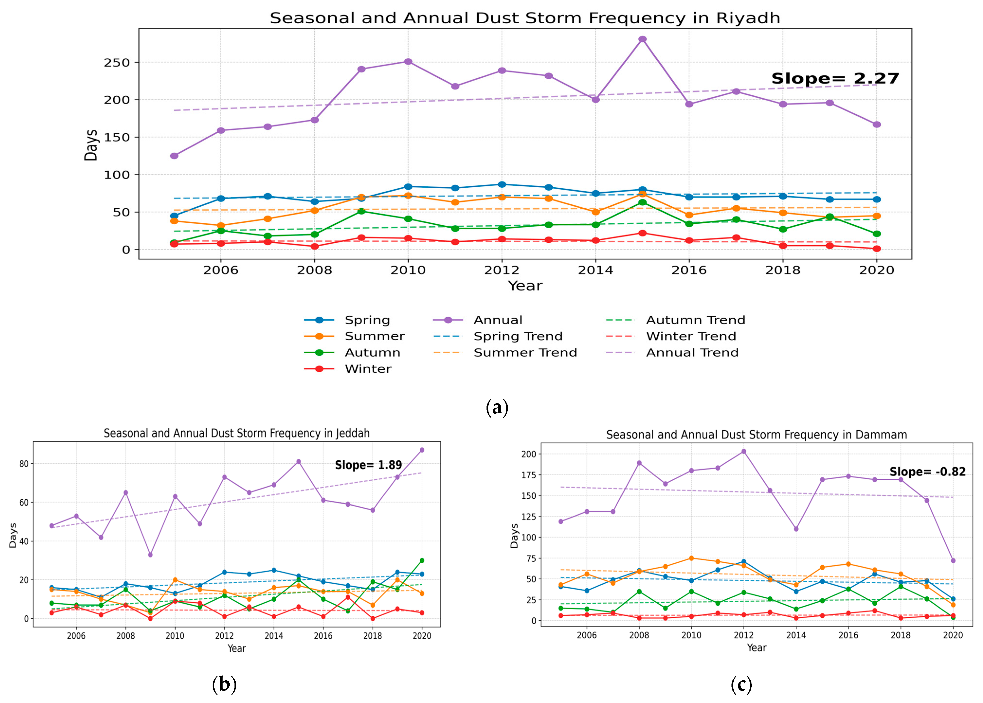
The analysis revealed significant spatial and seasonal variability in dust storm occurrences across Riyadh, Jeddah, and Dammam from 2005 to 2020, as shown in Figure 4a–c. We compiled the mean and standard deviation (SD) of dust storm frequencies into Table 5, which compares seasonal trends among the cities.
This overview highlights that Riyadh experiences the highest volume of dust storms, particularly in spring, with a mean of 72 events ± 10 SD, aligning with the broader regional pattern that sees increased dust storm frequencies during spring and summer [7,51,52]. Dammam also shows heightened dust storm activity during these seasons, reflecting regional climatic patterns. Contrastingly, Jeddah exhibits a lower frequency of dust storms throughout the year. In particular, during the spring, Jeddah experiences an average of 19 events ± 4 SD, significantly fewer than Riyadh’s peak season. This trend continues into summer, autumn, and winter, with Jeddah recording lower mean events of 13 ± 5 SD, 11 ± 7 SD, and 4 ± 3 SD, respectively.
3.2. Feature Selection
The analysis initially focused on identifying potential multicollinearity among the meteorological variables within all three cities. Variables exhibiting a high degree of correlation, as defined by a threshold value exceeding ±0.8, were earmarked for exclusion. The derived correlation matrix, which outlines these correlations, is depicted in Figure 5a. Subsequently, the feature selection was refined using random forest importance scores, with a preference for continuous meteorological variables. This step is summarized in Figure 5b. Of the 17 assessed features, 6 were excluded to address multicollinearity concerns.
For the seven identified dust sources, a similar approach assessed the correlations among identical meteorological variables across different sources. The correlations among these features were visualized in heat maps: temperature correlations are shown in Figure 6a, humidity in Figure 6b, precipitation in Figure 6c, and pressure in Figure 6d. Wind speed and direction were excluded from the exclusion criteria applied to other variables due to their direct effect on dust events.
Subsequently, the random forest method was utilized to refine the feature selection, removing one feature from each pair with a high correlation. From the 28 features initially analyzed, 18 were excluded to eliminate multicollinearity, with a particular focus on temperature (DS2, DS3, DS4, DS5, DS6, and DS7), humidity (DS1, DS2, DS3, DS4, DS5, and DS6), and pressure (DS1, DS2, DS3, DS4, DS6, and DS7) features. The importance of each feature to dust storm frequency and the excluded features are highlighted in red in Figure 6e.
In our study on Riyadh, Jeddah, and Dammam, we included three land cover features representing distinct classes, while excluding land cover data for all dust source areas due to the assumed minimal variability. Instead, we focused on the meteorological and vegetative factors more related to dust emissions in these areas. Additionally, we incorporated features such as seasonal variations, wind directions, windy days, and the previous month’s dust storm frequency directly into our model, thereby bypassing the initial feature selection. Their impact was evaluated using the SHAP values in Section 3.4. Ultimately, the features selected for the final model are detailed in Table A1 (Appendix A).
3.3. Comparison of the Results of Different Predicting Models
The comparative performance of the models employed to predict monthly dust storm frequency across three major cities in Saudi Arabia, Riyadh, Jeddah, and Dammam, is presented in Table 6. The models evaluated include MLR, SVR, GBRT, LSTM, TCN, and a persistence method used as a baseline for comparison; the accuracy matrices used are MAE, RMSE, and R2.
In Riyadh, which has more regular dust storm occurrences, the LSTM and TCN outperform traditional regression approaches, with R2 values of 0.50 and 0.51, respectively, indicating that they capture the complex temporal patterns of dust storms in the region. The negative R2 value for the persistence method suggests that this approach is insufficient for such dynamic weather events. For Jeddah, the task is more challenging, as indicated by the close performance metrics across the models. This complexity can be attributed to the coastal city’s variable climate, the influence of remote dust sources in Africa across the Red Sea [6], and the less frequent nature of dust storms. The LSTM model exhibits the lowest MAE and RMSE values, indicating its effectiveness in capturing long-term temporal dependencies within the aggregated data. Dammam also shows that the LSTM model demonstrates the highest R2 value of 0.64, suggesting a strong model fit. The models performed better in predicting dust storms for Riyadh due to the city’s more consistent and defined seasonal patterns, driven by its desert climate. The coastal climate and variable interactions in Jeddah and Dammam could introduce additional complexity in dust storm forecasting, thus affecting model accuracy.
Plotting the actual dust storm frequencies against the predictions made by each model over the test period from June 2016 to November 2020 shows the variability in their predictive capabilities across different time frames. Figure 7, Figure 8 and Figure 9 present the time series of actual dust storm frequencies alongside the corresponding predictions generated by each model over the test period from June 2016 to November 2020. The figures show the seasonal variations and annual trends, with peak frequencies observed during certain months, indicative of the cyclical nature of dust storm occurrences.
The LSTM model’s performance revealed a pattern of underestimating high-activity periods. In Riyadh (Figure 7), notable underpredictions occurred in early 2017 and December 2018, with a significant shortfall in December 2018, when the actual frequency spiked. In Jeddah (Figure 8), the LSTM fell short during unexpected events. Dammam (Figure 9) shows a similar trend despite occasional accurate predictions. The LSTM model requires refinement to improve its accuracy during peak activity periods.
The TCN model shows varied accuracy for predicting dust storm frequencies in Riyadh, Jeddah, and Dammam. In Riyadh, it closely captured higher-frequency events but tended to slightly overestimate them during other times, such as late 2019 and 2020. In Jeddah, the TCN model consistently underestimated the dust storm frequency, particularly in high-activity months (e.g., January and August 2020), indicating that it might not fully detect sudden spikes in dust storm activity. Dammam experienced similar underestimation issues with the TCN model, especially during peak periods. However, an exception occurred in 2020, which was a year marked by unusually lower activity, where the model tended to overestimate the frequency, highlighting a reversal in the trend of underestimation seen in other periods and cities.
The SVR model tended to overestimate Riyadh dust storm occurrences, particularly in periods of lower dust storm activity, as observed in late 2018 and early 2019. This suggests a bias in the model toward higher frequency predictions during periods of low activity. Conversely, in Jeddah, the SVR model consistently underestimated actual dust storm frequencies, notably during high-activity periods, such as August 2020, when it predicted significantly fewer storms than what occurred. This pattern of underestimation extends to Dammam, where the model similarly undervalued dust storm frequencies across various periods.
By contrast, the GBRT model demonstrated significant adaptability and responsiveness to changes. In Riyadh, the GBRT aligned with the actual dust storm frequency, accurately capturing the spike in December 2018 and the high-activity trends of early 2019; thus, these findings are consistent with the efficacy of the gradient-boosting techniques highlighted in previous studies [21,22,34]. In Jeddah, GBRT showcased an improved predictive capability, closely matching the actual frequencies in instances such as February and March 2020. However, it struggled with sudden increases in activity, similar to the SVR model, as seen in August 2020. Dammam’s results align with those of other cities, with its predictions closely matching actual occurrences, thereby demonstrating its capability to capture trends and peaks. This performance across the cities underscores GBRT’s potential in environmental forecasting, especially in capturing sudden events.
The MLR model’s performance varied, with a general tendency toward overprediction in some instances and underprediction in others. This variability underscores the challenges linear models face in capturing the complex, non-linear dynamics of dust storms. The predictions have a consistent pattern of overestimation across the entire period for Riyadh and Jeddah. Conversely, Dammam shows better results, but they still include underprediction and overprediction, reflecting MLR’s struggle with the complex factors driving dust storms. For that, the non-linear models (e.g., GBRT, TCN) provide a better fit.
Among the models analyzed, the GBRT and TCN models stand out for their precision in capturing high-frequency dust storm events. The TCN model exhibited a slight edge in accurately mirroring the actual data, particularly in forecasting the magnitude of the activity peaks. The LSTM model, while providing a smoother predictive curve, and the SVR model, with its conservative estimations, offered valuable insights into the trade-offs between capturing long-term trends and responding to immediate changes in dust storm activity.
The residuals for the LSTM and TCN models for Riyadh are presented in Figure 10, illustrating their predictive accuracy and error distributions. A complete set of residual visualizations across all evaluated models for all cities is in Appendix A, Figure A1, Figure A2 and Figure A3.
The residuals (i.e., the differences between the observed and prediction values) in Figure 10 highlight a generally low distribution, affirming their efficacy in accurately predicting dust storm occurrences for most of the evaluated period. However, the LSTM model shows a slightly broader range of positive residuals, which suggests instances in which it underpredicted actual events more so than the TCN model.
3.4. Assessing Feature Contributions Using SHAP Values
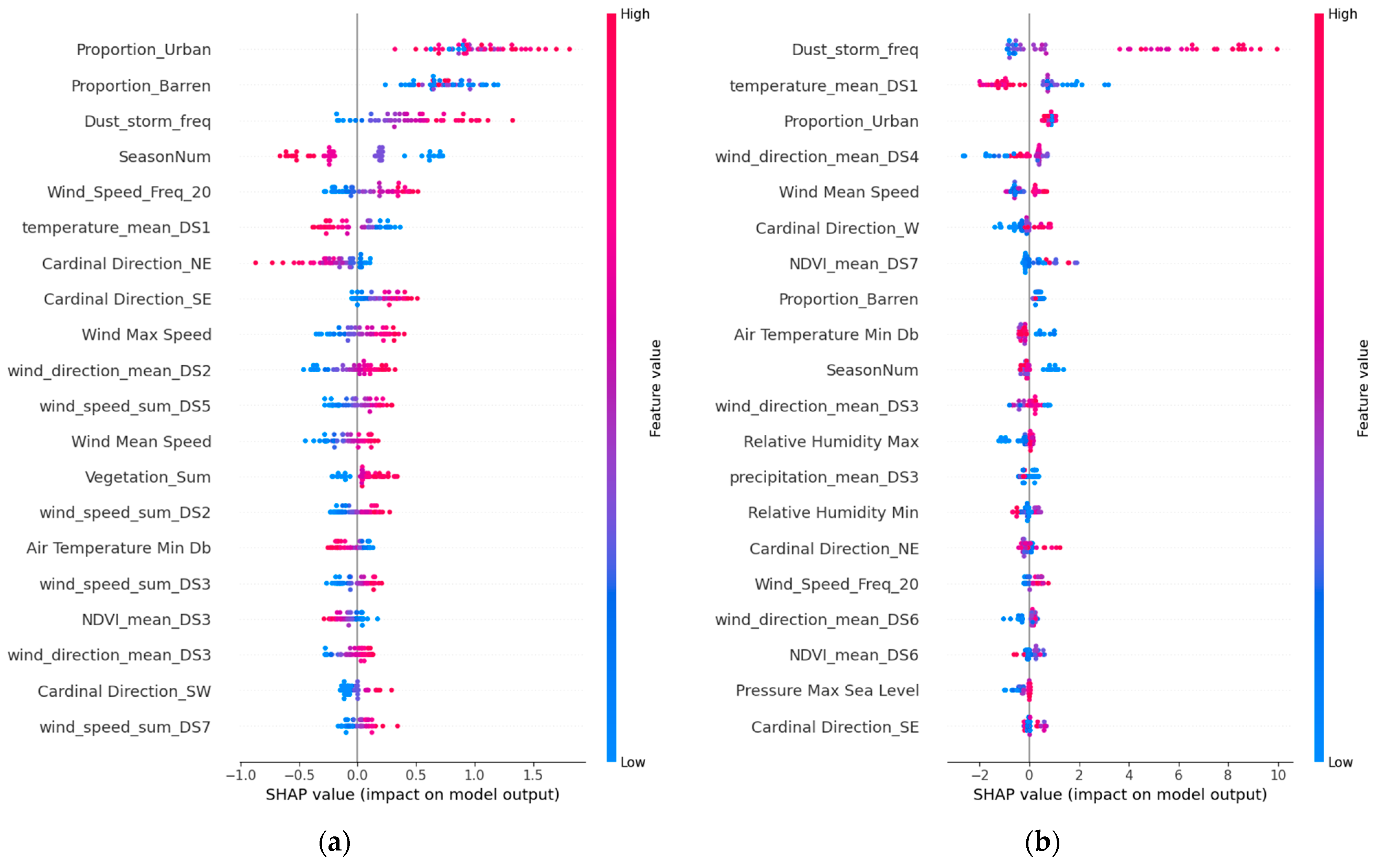
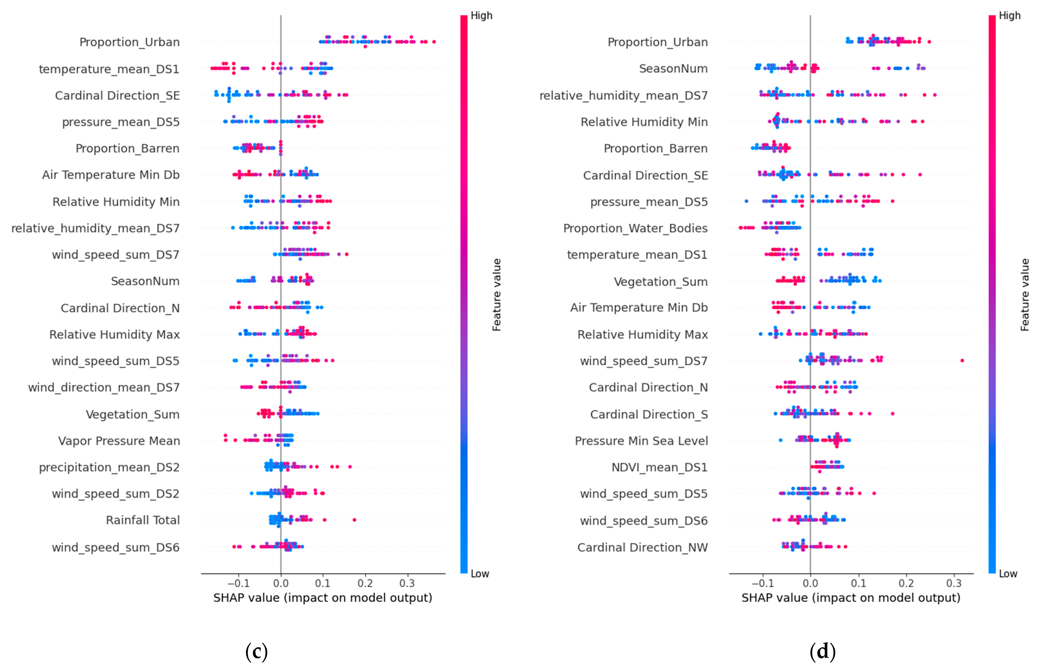
SHAP values help quantify the importance of various predictors in various models, such as SVR, GBRT, LSTM, and TCN (but excluding MLR due to its low performance). We aimed to understand how environmental features and specific dust sources affect model predictions. Among 62 predictors for forecasting dust storms, the top 20 were identified as significant. In Figure 11, Figure 12 and Figure 13, which analyze these predictors for Riyadh, Jeddah, and Dammam, the red dots indicate higher feature values, while the blue dots have lower values. Their position on the SHAP value axis reveals whether these features positively or negatively affected the predictions. This analysis shows the intricate relationships among the meteorological, urban, and vegetation factors in dust storm dynamics across the three cities.
Seasonal variations, denoted as “SeasonNum”, highlight the temporal variability in dust storm occurrences, suggesting that seasonal shifts in wind patterns are critical in initiating and transporting dust storms.
In Riyadh (Figure 10), the meteorological conditions and specific wind patterns from dust sources notably affect dust storm frequency. Features like “Air Temperature Min” (e.g., SHAP value: 0.33 in GBRT), specific wind directions, such as “NE” and “SE”, and wind directions from specific dust sources, such as “wind_direction_mean_DS4” (SHAP value: 0.66) and “wind_direction_mean_DS3” (SHAP value: 0.30) in GBRT, are pivotal. The wind speed, particularly the “Wind Mean Speed” and “Wind_Speed_Freq_20,” with SHAP values of 0.47 and 0.23, respectively, in GBRT, plays a significant role in prediction. The “wind_speed_sum_DS” feature, which is the sum of windy days with more than 20 km/h for areas like DS2, DS3, and DS6, especially in the TCN model, underlines the influence of wind speeds from these sources on dust storm occurrences.
Jeddah’s analysis (Figure 11) points to the significant roles of wind characteristics, including speed (“Wind Mean Speed”, with a SHAP value of 0.201 in GBRT) and wind direction from dust sources (“wind_direction_mean_DS5” at 0.314 and “wind_direction_mean_DS7” at 0.291 in GBRT), as crucial in influencing dust patterns. The SVR, LSTM and TCN models also reflect the importance of these factors, although they have varying degrees of impact, indicating a complex interplay among the factors.
Meteorological and wind-related factors similarly influenced Dammam’s pattern (Figure 12). The key features include “Air Temperature Min” with a SHAP value of 0.33 in the GBRT model. Wind direction in dust sources, particularly “wind_direction_mean_DS2” (0.66 SHAP value) and “wind_direction_mean_DS3” (0.30 SHAP value), in the GBRT model. Wind speed factors like “Wind Mean Speed” (0.47 SHAP value) and “Wind_Speed_Freq_20” (0.23 SHAP value) also play a critical role in the prediction output.
The analyses of Riyadh, Jeddah, and Dammam also emphasize the impact of the relative humidity, precipitation, and urban and barren lands on dust activity. Urban areas, particularly in Riyadh and Jeddah, alongside barren lands, significantly affect dust storm dynamics. These findings highlight the complex influences of environmental, urban, and vegetative factors on dust storm patterns, underscoring the importance of integrating these elements into predictive models for effective forecasting and mitigation strategies. The greatest impact on urban areas was observed in the SVR model for Riyadh (SHAP value: 1.02) and barren areas in the GBRT model (SHAP value: 0.75), highlighting the critical roles of urbanization and land surface conditions in influencing dust storm occurrences. A previous study [5] identified urbanization as a key driver of changing dust storm patterns in Saudi Arabia, supporting our findings regarding the need to consider urban expansion and natural land conditions in dust storm frequency analysis. Further support for the influence of barren areas on dust storm activity in the study by [17] corroborates our findings by showing how drying wetlands and expanding barren lands amplify dust occurrence.
The vegetation dynamics offer contrasting insights. The “Vegetation_Sum” feature, which includes croplands, herbaceous areas, and shrublands, shows a positive correlation with dust storm frequency in our models for Riyadh, with the highest SHAP value observed in the GBRT model (SHAP value: 0.80). This suggests that areas with heavier vegetation, potentially reflecting intensive agricultural activities on cropland, may contribute to dust storm occurrences, likely due to soil disturbance and reduced soil moisture, which turn these areas into dust sources, as reported previously [53]. Conversely, the “NDVI_mean” feature demonstrates a negative correlation with dust storm frequency, indicating that increased vegetation health and density, as captured by higher NDVI values, can mitigate dust storm activity. The greatest negative impact of the NDVI on dust storm frequency was observed in the GBRT model for Jeddah (SHAP value: −0.64), suggesting that healthier vegetation cover plays a crucial role in stabilizing soils and reducing dust emissions. Therefore, the health and density of vegetation within identified dust source areas, such as “NDVI_mean_DS7” and “NDVI_mean_DS3”, inversely affect dust storm frequency. Similarly, for Dammam, GBRT underscores NDVI_mean_DS3 with a SHAP value of 0.49 and NDVI_mean_DS1 with a SHAP value of 0.23, suggesting NDVI’s substantial role, as mentioned in [54,55].
This analysis explains the complex interplay between meteorological, environmental conditions, urbanization, and dust sources that influence dust storm frequency. It underscores the need for integrated dust storm management strategies that consider urban planning, vegetation cover enhancement, and targeted mitigation efforts based on seasonal and meteorological factors.
4. Conclusions
This research developed the forecasting of dust storm frequencies in three cities of Saudi Arabia—Riyadh, Jeddah, and Dammam—by integrating meteorological and environmental variables, NDVI, land use data, and characteristics of dust sources with various machine learning and deep learning models. The results highlight the effectiveness of the LSTM and TCN models in capturing the complex temporal dynamics of dust storms and demonstrate that they outperform traditional methods, as evidenced by their lower MAE and RMSE values and higher R2 scores.
The TCN model showcased its remarkable performance in Riyadh, with an R2 score of 0.51, an MAE of 2.80, and an RMSE of 3.48, highlighting its precision and adaptability to the city’s specific environmental and climatic conditions. Conversely, in Dammam, the LSTM model proved to be the most accurate, achieving an MAE of 3.02, an RMSE of 3.64, and an outstanding R2 score of 0.64. In Jeddah, the LSTM model also exhibited a competitive edge, achieving an MAE of 2.48 and an RMSE of 2.96.
The utilization of SHAP value analysis revealed the considerable impact of seasonality, wind-related features, and environmental factors, such as the NDVI, vegetation cover, urban and barren land use, and specific dust source characteristics, in predicting dust storm frequency.
This research shows the potential of using deep learning models to improve the accuracy and reliability of dust storm frequency forecasts with the sliding window technique for historical months. It ultimately demonstrates integrating advanced machine learning techniques with detailed environmental data as a promising approach to improving the understanding and prediction of complex meteorological events.
Author Contributions
Conceptualization, R.K.A., O.A. and M.S.A.; methodology, R.K.A.; writing—review and editing, R.K.A., O.A. and M.S.A.; supervision, O.A. and M.S.A. All authors have read and agreed to the published version of the manuscript.
Funding
This research received no external funding.
Institutional Review Board Statement
Not applicable.
Informed Consent Statement
Not applicable.
Data Availability Statement
Publicly available datasets were analyzed in this study. These datasets can be found here: Meteorological data: https://power.larc.nasa.gov/data-access-viewer/ (accessed on 25 May 2023), land cover: https://developers.google.com/earth-engine/datasets/catalog/MODIS_061_MCD12Q1, (accessed on 1 July 2023) and NDVI: https://developers.google.com/earth-engine/datasets/catalog/MODIS_061_MOD13A2, (accessed on 1 July 2023).
Acknowledgments
The authors would like to thank the Scientific Research at King Saud University for their support of this research. We also extend our thanks to King Abdulaziz City for Science and Technology (KACST) for their contributions and support.
Conflicts of Interest
The authors declare no conflicts of interest.
Appendix A

Table A1.
Selected Meteorological and Environmental Features with their corresponding count, description, and units.
Table A1.
Selected Meteorological and Environmental Features with their corresponding count, description, and units.
| Feature | Number of Features | Description | Units |
|---|---|---|---|
| Wind Direction | 10 | These features are binary indicators representing the presence or absence of wind from specific directions. “Calm” signifies no wind, while the other labels (E, N, NE, NW, S, SE, SW, W) denote wind from the east, north, northeast, northwest, south, southeast, southwest, and west, respectively. “Variable” indicates changing wind directions. | 0 or 1 |
| Pressure Max Sea Level | 1 | Maximum atmospheric pressure at sea level. | hPa |
| Wind Max Speed | 1 | Maximum wind speed recorded during the observation period. | km/h |
| Vapor Pressure Mean | 1 | Average vapor pressure in the air. | hPa |
| Wind Mean Speed | 1 | Average wind speed recorded during the observation period. | km/h |
| Pressure Min Sea Level | 1 | Minimum atmospheric pressure at sea level. | hPa |
| Air Temperature Min | 1 | Minimum dry-bulb air temperature recorded. | °C |
| Pressure Max Station Level | 1 | Maximum atmospheric pressure recorded at the station level. | hPa |
| Relative Humidity Min | 1 | Minimum relative humidity recorded during the observation period. | % |
| Rainfall Total | 1 | Total rainfall recorded during the observation period. | mm |
| Relative Humidity Max | 1 | Maximum relative humidity recorded during the observation period. | % |
| Dust_storm_freq | 1 | Frequency of dust storm events within the observation period. | days |
| SeasonNum | 1 | Numeric representation of the season (1–4). | categorical |
| Wind Speed Sum at Dust Sources | 7 | Cumulative wind speeds measured at seven different dust sources (DS1 to DS7). This encompasses the aggregated days of wind speeds above 20 km/h at each dust source. | days |
| Wind_Speed_Freq_20 | 1 | Frequency of wind speed occurrences above 20 km/h. | days |
| Relative Humidity Mean at DS7 | 1 | Average relative humidity measured at dust source 7. | % |
| Temperature Mean at DS1 | 1 | Average temperature measured at dust source 1. | °C |
| Precipitation Mean at DS1 to DS7 | 7 | Average precipitation measured at dust sources 1 to 7, indicating moisture levels that could impact dust mobilization. | mm |
| Pressure Mean at DS5 | 1 | Average atmospheric pressure measured at dust source 5. | hPa |
| Wind Direction Mean at DS1 to DS7 | 7 | Average wind direction measured at dust sources 1 to 7, indicating predominant wind directions at each source. | ° |
| Proportions of Land Cover Types | 3 | Proportions of barren land, water bodies, and urban areas within the study region. | % |
| Vegetation Sum | 1 | Sum of vegetation coverage, indicating proportion of natural herbaceous, shrublands, and herbaceous croplands. | % |
| NDVI and NDVI Mean at DS1 to DS7 | 8 | Normalized difference vegetation index and its average values at dust sources 1 to 7, assessing vegetation health. | Index (0–1) |
| Total Number of Features | 61 |
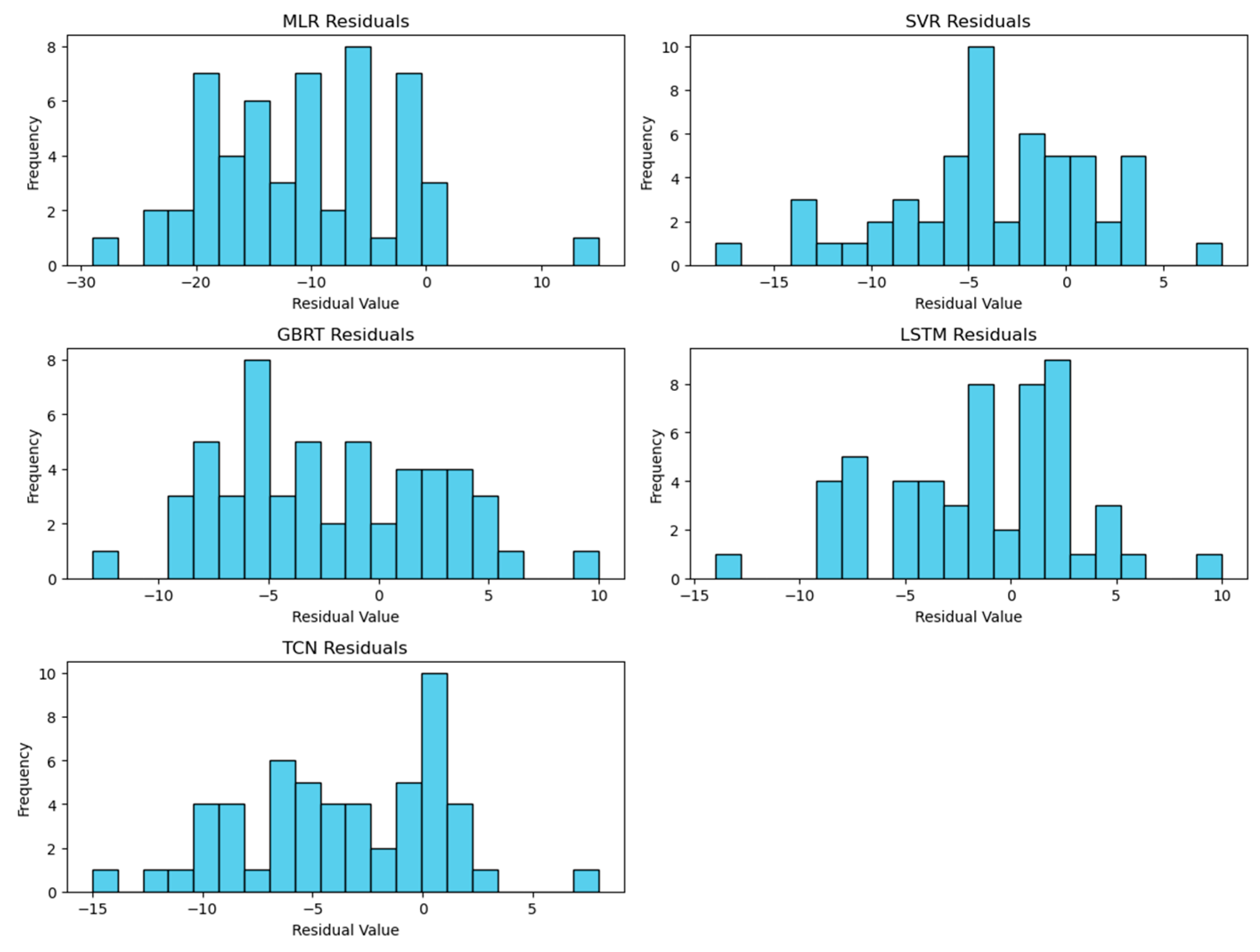
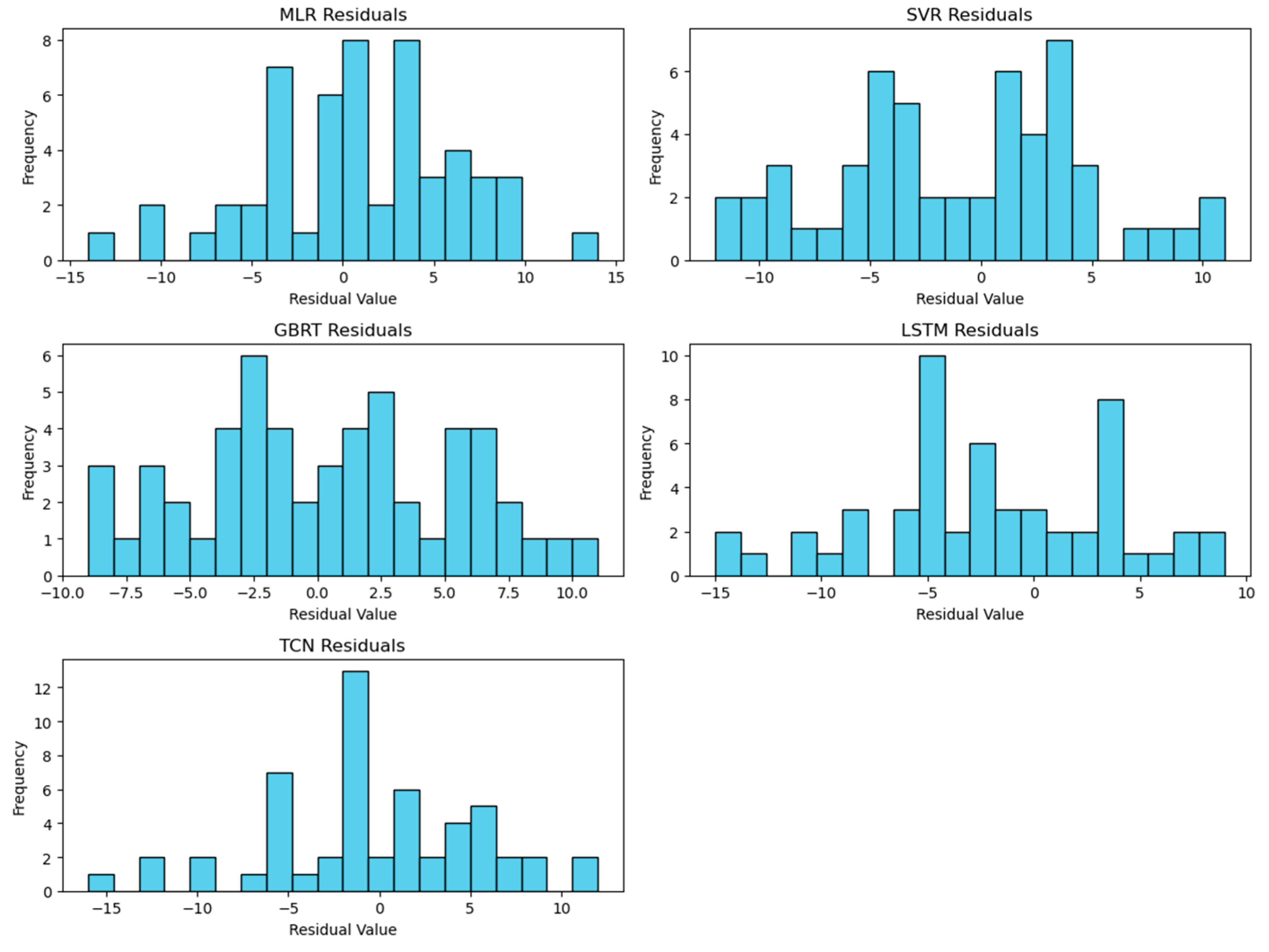
The residual distributions for all models in Figure A1, Figure A2 and Figure A3 provide a detailed visualization of the residual distributions for each of the five models (MLR, SVR, GBRT, LSTM, and TCN) evaluated in our study across the three cities. These visualizations offer the variability and prediction errors of each model.
Figure A1.
Residual distributions for all predictive models in Riyadh.

Figure A2.
Residual distributions for all predictive models in Jeddah.

Figure A3.
Residual distributions for all predictive models in Dammam.

References
- Middleton, N.; Kang, U. Sand and Dust Storms: Impact Mitigation. Sustainability 2017, 9, 1053. [Google Scholar] [CrossRef]
- Furman, H.K.H. Dust Storms in the Middle East: Sources of Origin and Their Temporal Characteristics. Indoor Built Environ. 2003, 12, 419–426. [Google Scholar] [CrossRef]
- Al-Dousari, A.M.; Al-Awadhi, J.; Ahmed, M. Dust Fallout Characteristics within Global Dust Storm Major Trajectories. Arab. J. Geosci. 2013, 6, 3877–3884. [Google Scholar] [CrossRef]
- Shepherd, G.; Terradellas, E.; Baklanov, A.; Kang, U.; Sprigg, K.; Nickovic, S.; Boloorani, A.; Al-Dousari, A.; Basart, S.; Benedetti, A. Global Assessment of Sand and Dust Storms; United Nations Environment Programme (UNEP): Nairobi, Kenya, 2016; ISBN 978-92-807-3551-2. [Google Scholar]
- Notaro, M.; Alkolibi, F.; Fadda, E.; Bakhrjy, F. Trajectory Analysis of Saudi Arabian Dust Storms. J. Geophys. Res. Atmospheres 2013, 118, 6028–6043. [Google Scholar] [CrossRef]
- Alharbi, B.H. Airborne Dust in Saudi Arabia: Source Areas, Entrainment, Simulation and Composition. Ph.D. Dissertation, Monash University, Clayton, VIC, Australia, 2009. [Google Scholar]
- Albugami, S.; Palmer, S.; Cinnamon, J.; Meersmans, J. Spatial and Temporal Variations in the Incidence of Dust Storms in Saudi Arabia Revealed from In Situ Observations. Geosciences 2019, 9, 162. [Google Scholar] [CrossRef]
- McCabe, M.; AlShalan, M.; Hejazi, M.; Beck, H.; Maestre, F.T.; Guirado, E.; Peixoto, R.S.; Duarte, C.M.; Wada, Y.; Al-Ghamdi, S.; et al. Climate Futures Report: Saudi Arabia in a 3 Degrees Warmer World; KAUST, AEON Collective, KAPSARC: Jeddah, Saudi Arabia, 2023. [Google Scholar] [CrossRef]
- Akhlaq, M.; Sheltami, T.R.; Mouftah, H.T. A Review of Techniques and Technologies for Sand and Dust Storm Detection. Rev. Environ. Sci. Biotechnol. 2012, 11, 305–322. [Google Scholar] [CrossRef]
- Peltier, R.E.; Castell, N.; Clements, A.L.; Dye, T.; Hüglin, C.; Kroll, J.H.; Lung, S.-C.C.; Ning, Z.; Parsons, M.; Penza, M. An Update on Low-Cost Sensors for the Measurement of Atmospheric Composition, December 2020; World Meteorological Organization: Geneva, Switzerland, 2021. [Google Scholar]
- WMO. Manual on Codes, Volume I.1—International Codes; WMO-No. 306; WMO: Geneva, Switzerland, 1974. [Google Scholar]
- Dar, M.A.; Ahmed, R.; Latif, M.; Azam, M. Climatology of Dust Storm Frequency and Its Association with Temperature and Precipitation Patterns over Pakistan. Nat. Hazards 2022, 110, 655–677. [Google Scholar] [CrossRef]
- Middleton, N.J.; Goudie, A.S. Saharan Dust: Sources and Trajectories. Trans. Inst. Br. Geogr. 2001, 26, 165–181. [Google Scholar] [CrossRef]
- Alshammari, R.K.; Alrwais, O.; Aksoy, M.S. Machine Learning Applications to Dust Storms: A Meta-Analysis. Aerosol Air Qual. Res. 2022, 22, 220183. [Google Scholar] [CrossRef]
- Ali, M.; Asklany, S.A.; El-wahab, M.; Hassan, M. Data Mining Algorithms for Weather Forecast Phenomena Comparative Study. Int. J. Comput. Sci. Netw. Secur. 2019, 19, 76–81. [Google Scholar]
- Al Murayziq, T.S.; Kapetanakis, S.; Petridis, M. Intelligent Signal Processing for Dust Storm Prediction Using Ensemble Case-Based Reasoning. In Proceedings of the 2017 IEEE 29th International Conference on Tools with Artificial Intelligence (ICTAI), Boston, MA, USA, 6–8 November 2017; pp. 1267–1271. [Google Scholar]
- Shaiba, H.A.; Alaashoub, N.S.; Alzahrani, A.A. Applying Machine Learning Methods for Predicting Sand Storms. In Proceedings of the 2018 1st International Conference on Computer Applications & Information Security (ICCAIS), Riyadh, Saudi Arabia, 4–6 April 2018; pp. 1–5. [Google Scholar]
- Aryal, Y. Evaluation of Machine-Learning Models for Predicting Aeolian Dust: A Case Study over the Southwestern USA. Climate 2022, 10, 78. [Google Scholar] [CrossRef]
- Aryal, Y. Application of Artificial Intelligence Models for Aeolian Dust Prediction at Different Temporal Scales: A Case with Limited Climatic Data. AI 2022, 3, 707–718. [Google Scholar] [CrossRef]
- Zhang, Z.; Ma, C.; Xu, J.; Huang, J.; Li, L. A Novel Combinational Forecasting Model of Dust Storms Based on Rare Classes Classification Algorithm. In Geo-Informatics in Resource Management and Sustainable Ecosystem; Springer: Berlin/Heidelberg, Germany, 2014; pp. 520–537. [Google Scholar]
- Ebrahimi-Khusfi, Z.; Dargahian, F.; Nafarzadegan, A.R. Predicting the Dust Events Frequency around a Degraded Ecosystem and Determining the Contribution of Their Controlling Factors Using Gradient Boosting-Based Approaches and Game Theory. Environ. Sci. Pollut. Res. Int. 2022, 29, 36655–36673. [Google Scholar] [CrossRef] [PubMed]
- Ebrahimi-khusfi, Z.; Nafarzadegan, A.R.; Dargahian, F. Predicting the Number of Dusty Days around the Desert Wetlands in Southeastern Iran Using Feature Selection and Machine Learning Techniques. Ecol. Indic. 2021, 125, 107499. [Google Scholar] [CrossRef]
- Nabavi, S.O.; Haimberger, L.; Abbasi, R.; Samimi, C. Prediction of Aerosol Optical Depth in West Asia Using Deterministic Models and Machine Learning Algorithms. Aeolian Res. 2018, 35, 69–84. [Google Scholar] [CrossRef]
- Ebrahimi-khusfi, Z.; Taghizadeh-Mehrjardi, R.; Mirakbari, M. Evaluation of Machine Learning Models for Predicting the Temporal Variations of Dust Storm Index in Arid Regions of Iran. Atmos. Pollut. Res. 2021, 12, 134–147. [Google Scholar] [CrossRef]
- Ebrahimi Khusfi, Z.; Roustaei, F.; Ebrahimi Khusfi, M.; Naghavi, S. Investigation of the Relationship between Dust Storm Index, Climatic Parameters, and Normalized Difference Vegetation Index Using the Ridge Regression Method in Arid Regions of Central Iran. Arid Land Res. Manag. 2020, 34, 239–263. [Google Scholar] [CrossRef]
- NASA Langley Research Center Power Data Access Viewer. Available online: https://power.larc.nasa.gov/data-access-viewer/ (accessed on 25 May 2023).
- NASA LP DAAC at the USGS EROS Center. MCD12Q1.061 MODIS Land Cover Type Yearly Global 500 m. Available online: https://developers.google.com/earth-engine/datasets/catalog/MODIS_061_MCD12Q1 (accessed on 1 July 2023).
- NASA LP DAAC at the USGS EROS Center. MOD13A2.061 Terra Vegetation Indices 16-Day Global 1 km. Available online: https://developers.google.com/earth-engine/datasets/catalog/MODIS_061_MOD13A2 (accessed on 1 July 2023).
- Gholami, H.; Mohamadifar, A.; Sorooshian, A.; Jansen, J.D. Machine-Learning Algorithms for Predicting Land Susceptibility to Dust Emissions: The Case of the Jazmurian Basin, Iran. Atmos. Pollut. Res. 2020, 11, 1303–1315. [Google Scholar] [CrossRef]
- Sarasa-Cabezuelo, A. Prediction of Rainfall in Australia Using Machine Learning. Information 2022, 13, 163. [Google Scholar] [CrossRef]
- Xu, C.; Guan, Q.; Lin, J.; Luo, H.; Yang, L.; Tan, Z.; Wang, Q.; Wang, N.; Tian, J. Spatiotemporal Variations and Driving Factors of Dust Storm Events in Northern China Based on High-Temporal-Resolution Analysis of Meteorological Data (1960–2007). Env. Pollut. 2020, 260, 114084. [Google Scholar] [CrossRef]
- Barrera-Animas, A.Y.; Oyedele, L.O.; Bilal, M.; Akinosho, T.D.; Delgado, J.M.D.; Akanbi, L.A. Rainfall Prediction: A Comparative Analysis of Modern Machine Learning Algorithms for Time-Series Forecasting. Mach. Learn. Appl. 2022, 7, 100204. [Google Scholar] [CrossRef]
- Niu, D.; Wang, K.; Sun, L.; Wu, J.; Xu, X. Short-Term Photovoltaic Power Generation Forecasting Based on Random Forest Feature Selection and CEEMD: A Case Study. Appl. Soft Comput. 2020, 93, 106389. [Google Scholar] [CrossRef]
- An, H.; Li, Q.; Lv, X.; Li, G.; Qian, Q.; Zhou, G.; Nie, G.; Zhang, L.; Zhu, L. Forecasting Daily Extreme Temperatures in Chinese Representative Cities Using Artificial Intelligence Models. Weather Clim. Extrem. 2023, 42, 100621. [Google Scholar] [CrossRef]
- Schoof, J.T.; Pryor, S.C. Downscaling Temperature and Precipitation: A Comparison of Regression-Based Methods and Artificial Neural Networks. Int. J. Climatol. 2001, 21, 773–790. [Google Scholar] [CrossRef]
- Kean Hua, A. Applied Chemometric Approach in Identification Sources of Air Quality Pattern in Selangor, Malaysia. Sains Malays. 2018, 47, 471–479. [Google Scholar] [CrossRef]
- Preece, D.A.; Holder, R.L. Multiple Regression in Hydrology. Statistician 1986, 35, 566. [Google Scholar] [CrossRef]
- Cortes, C.; Vapnik, V. Support-Vector Networks. Mach. Learn. 1995, 20, 273–297. [Google Scholar] [CrossRef]
- Rivas-Perea, P.; Rivas-Perea, P.E.; Cota-Ruiz, J.; Aragon Franco, R. Near Real-Time Dust Aerosol Detection with Support Vector Machines for Regression. In Proceedings of the American Geophysical Union, Fall Meeting 2015, San Francisco, CA, USA, 14–18 December 2015; Volume 2015, p. A23C-033123. [Google Scholar]
- Friedman, J.H. Greedy Function Approximation: A Gradient Boosting Machine. Ann. Stat. 2001, 29, 1189–1232. [Google Scholar] [CrossRef]
- Hochreiter, S.; Schmidhuber, J. Long Short-Term Memory. Neural Comput. 1997, 9, 1735–1780. [Google Scholar] [CrossRef]
- Bai, S.; Kolter, J.Z.; Koltun, V. An Empirical Evaluation of Generic Convolutional and Recurrent Networks for Sequence Modeling. arXiv 2018, arXiv:1803.01271. [Google Scholar] [CrossRef]
- Zha, W.; Liu, J.; Li, Y.; Liang, Y. Ultra-Short-Term Power Forecast Method for the Wind Farm Based on Feature Selection and Temporal Convolution Network. ISA Trans. 2022, 129, 405–414. [Google Scholar] [CrossRef]
- Pedregosa, F.; Varoquaux, G.; Gramfort, A.; Michel, V.; Thirion, B.; Grisel, O.; Blondel, M.; Prettenhofer, P.; Weiss, R.; Dubourg, V. Scikit-Learn: Machine Learning in Python. J. Mach. Learn. Res. 2011, 12, 2825–2830. [Google Scholar]
- Thanh Ngoc, T.; Van Dai, L.; Minh Thuyen, C. Support Vector Regression Based on Grid Search Method of Hyperparameters for Load Forecasting. Acta Polytech. Hung. 2021, 18, 143–158. [Google Scholar] [CrossRef]
- Yao, J.; Cai, Z.; Qian, Z.; Yang, B. A Noval Approach Based on TCN-LSTM Network for Predicting Waterlogging Depth with Waterlogging Monitoring Station. PLoS ONE 2023, 18, e0286821. [Google Scholar] [CrossRef]
- Roberts, D.R.; Bahn, V.; Ciuti, S.; Boyce, M.S.; Elith, J.; Guillera-Arroita, G.; Hauenstein, S.; Lahoz-Monfort, J.J.; Schröder, B.; Thuiller, W.; et al. Cross-Validation Strategies for Data with Temporal, Spatial, Hierarchical, or Phylogenetic Structure. Ecography 2017, 40, 913–929. [Google Scholar] [CrossRef]
- Lundberg, S.; Lee, S.-I. A Unified Approach to Interpreting Model Predictions. arXiv 2017, arXiv:1705.07874. [Google Scholar] [CrossRef]
- Boroughani, M.; Pourhashemi, S.; Gholami, H.; Kaskaoutis, D.G. Predicting of Dust Storm Source by Combining Remote Sensing, Statistic-Based Predictive Models and Game Theory in the Sistan Watershed, Southwestern Asia. J. Arid Land 2021, 13, 1103–1121. [Google Scholar] [CrossRef]
- Gholami, H.; Mohammadifar, A.; Malakooti, H.; Esmaeilpour, Y.; Golzari, S.; Mohammadi, F.; Li, Y.; Song, Y.; Kaskaoutis, D.G.; Fitzsimmons, K.E.; et al. Integrated Modelling for Mapping Spatial Sources of Dust in Central Asia—An Important Dust Source in the Global Atmospheric System. Atmos. Pollut. Res. 2021, 12, 101173. [Google Scholar] [CrossRef]
- Yu, Y.; Notaro, M.; Kalashnikova, O.V.; Garay, M.J. Climatology of Summer Shamal Wind in the Middle East: Summer Shamal Climatology. J. Geophys. Res. Atmos. 2016, 121, 289–305. [Google Scholar] [CrossRef]
- Al-Misnad, A.; Al-Otaibi, M. Characteristics of the Bawarih Winds Blowing Over the Kingdom of Saudi Arabia. J. Arab Sci. Hum. 2017, 10. (In Arabic) [Google Scholar]
- FAO. Sand and Dust Storms; FAO: Rome, Italy, 2023; ISBN 978-92-5-138219-6. [Google Scholar]
- Halos, S.H.; Abed, F.G. Effect of Spring Vegetation Indices NDVI & EVI on Dust Storms Occurrence in Iraq. AIP Conf. Proc. 2019, 2144, 040015. [Google Scholar] [CrossRef]
- Li, J.; Garshick, E.; Al-Hemoud, A.; Huang, S.; Koutrakis, P. Impacts of Meteorology and Vegetation on Surface Dust Concentrations in Middle Eastern Countries. Sci. Total Environ. 2020, 712, 136597. [Google Scholar] [CrossRef] [PubMed]
Figure 1.
Location of the study area with the selected local dust sources. Each color defines a region.
Figure 1.
Location of the study area with the selected local dust sources. Each color defines a region.

Figure 2.
LSTM cell structure.

Figure 3.
The structure of the dilated causal convolution and the TCN residual block (kernel size of k = 3). Consistent shading across layers signifies their functionalities, while the detailed view displays the data as interconnected circles. A highlighted circle emphasizes the input and output, illustrating how data flows through the network.

Figure 4.
Time series analysis of dust storm frequencies in (a) Riyadh, (b) Jeddah, and (c) Dammam (2005–2020).
Figure 4.
Time series analysis of dust storm frequencies in (a) Riyadh, (b) Jeddah, and (c) Dammam (2005–2020).

Figure 5.
Meteorological features. (a) Correlation analysis, and (b) random forest feature importance. Exclusion of multicollinear features highlighted in red.
Figure 5.
Meteorological features. (a) Correlation analysis, and (b) random forest feature importance. Exclusion of multicollinear features highlighted in red.

Figure 6.
DS meteorological feature correlation analysis. (a) Temperature, (b) humidity, (c) precipitation, and (d) pressure. (e) Random forest feature importance; exclusion of multicollinear DS features highlighted in red.
Figure 6.
DS meteorological feature correlation analysis. (a) Temperature, (b) humidity, (c) precipitation, and (d) pressure. (e) Random forest feature importance; exclusion of multicollinear DS features highlighted in red.


Figure 7.
Differences between the predictions and observations using the LSTM, TCN, SVR, GBRT, and MLR models for Riyadh city.
Figure 7.
Differences between the predictions and observations using the LSTM, TCN, SVR, GBRT, and MLR models for Riyadh city.

Figure 8.
Differences between the predictions and observations using the LSTM, TCN, SVR, GBRT, and MLR models for Jeddah city.
Figure 8.
Differences between the predictions and observations using the LSTM, TCN, SVR, GBRT, and MLR models for Jeddah city.

Figure 9.
Differences between the predictions and observations using the LSTM, TCN, SVR, GBRT, and MLR models for Dammam city.
Figure 9.
Differences between the predictions and observations using the LSTM, TCN, SVR, GBRT, and MLR models for Dammam city.

Figure 10.
Residual distributions for LSTM and TCN for Riyadh.

Figure 11.
The Shaley additive explanations for the top 20 significant factors in Riyadh: (a) SVR; (b) GBRT; (c) LSTM; (d) TCN.
Figure 11.
The Shaley additive explanations for the top 20 significant factors in Riyadh: (a) SVR; (b) GBRT; (c) LSTM; (d) TCN.


Figure 12.
The Shapley additive explanations for the top 20 significant factors in Jeddah: (a) SVR; (b) GBRT; (c) LSTM; (d) TCN.
Figure 12.
The Shapley additive explanations for the top 20 significant factors in Jeddah: (a) SVR; (b) GBRT; (c) LSTM; (d) TCN.


Figure 13.
The Shaley additive explanations for the top 20 significant factors in Dammam: (a) SVR; (b) GBRT; (c) LSTM; (d) TCN.
Figure 13.
The Shaley additive explanations for the top 20 significant factors in Dammam: (a) SVR; (b) GBRT; (c) LSTM; (d) TCN.


Table 1.
Data source details.
| Dataset | Spatial/Temporal Resolutions | Temporal Coverage | Dataset Source |
|---|---|---|---|
| City: Meteorological Data | City/Daily | 2005–2020 | Saudi National Center for Meteorology |
| Dust Source: Meteorological Data | City/Daily | 2005–2020 | POWER/MERRA-2 Dataset |
| City/Dust Source: NDVI | 1 Km/16 Days | 2005–2020 | MODIS |
| City: Land Cover | 500 m/Yearly | 2005–2020 | MODIS |
Table 2.
Hyperparameters for SVR and GBRT models used in grid search optimization.
| Model | Hyperparameter | Values | Optimal Values |
|---|---|---|---|
| SVR | Kernel | [‘linear’, ‘rbf’, ‘sigmoid’] | Linear |
| C (regularization parameter) | [0.01, 0.1, 1, 10] | 0.001 | |
| Gamma (kernel coefficient) | [0.01, 0.1, 1, 10, 100, 1000] | 0.001 | |
| GBRT | Number of estimators | [10, 50, 100, 500] | 500 |
| Learning rate | [0.0001, 0.001, 0.01, 0.1, 1.0] | Of 0.1 | |
| Max depth | [3, 7, 9] | 3 |
Table 3.
Hyperparameter values for LSTM and TCN.
| Hyperparameter | LSTM | TCN |
|---|---|---|
| Window size | 1–20 | 1–20 |
| Number of layers | 1–4 | 1–4 |
| Number of nodes | 200, 150, 100, 50 | - |
| Training epochs | 12, 24, 50, 100 | 12, 24, 50, 100 |
| Batch size | 32, 64 | 32, 64 |
| Kernel size | - | 2, 5 |
| Learning rate | 0.001 | 0.001 |
| Dilation | - | 1, 2, 4, 8 |
Table 4.
Structure of LSTM and TCN after a grid search.
| Parameter | LTSM | TCN |
|---|---|---|
| Window size | 5 | 5 |
| Number of layers | 1 | 3 |
| Number of nodes | 200 | - |
| Training epochs | 24 | 100 |
| Batch size | 32 | 32 |
| Kernel size | - | 5 |
| Learning rate | 0.001 | 0.001 |
| Fully connected layer units | 50 | 50 |
| Fully connected layer units | 30 | 30 |
| Fully connected layer units | 20 | 20 |
Table 5.
Seasonal mean ± SD of dust storm frequencies in our study area (2005–2020).
| City | Spring (Days) | Summer (Days) | Autumn (Days) | Winter (Days) |
|---|---|---|---|---|
| Riyadh | 72 ± 10 | 54 ± 13 | 32 ± 13 | 11 ± 5 |
| Jeddah | 19 ± 4 | 13 ± 5 | 11 ± 7 | 4 ± 3 |
| Dammam | 48 ± 11 | 55 ± 6 | 14 ± 11 | 6 ± 3 |
Table 6.
Accuracy metrics for the test dataset for the three cities.
| City | MLR | SVR | GRBT | LSTM | TCN | Persistence | |
|---|---|---|---|---|---|---|---|
| Riyadh | MAE | 6.95 | 2.93 | 3.38 | 2.76 | 2.80 | 4.72 |
| RMSE | 8.36 | 3.60 | 3.87 | 3.52 | 3.48 | 5.81 | |
| R2 | −1.84 | 0.47 | 0.33 | 0.50 | 0.51 | −0.38 | |
| Jeddah | MAE | 2.87 | 2.49 | 2.56 | 2.48 | 2.61 | 2.79 |
| RMSE | 3.32 | 3.05 | 3.32 | 2.96 | 3.10 | 3.67 | |
| R2 | −0.12 | 0.11 | 0.01 | 0.12 | 0.02 | −0.29 | |
| Dammam | MAE | 4.68 | 3.63 | 3.92 | 3.02 | 3.44 | 10.03 |
| RMSE | 5.68 | 4.68 | 5.21 | 3.64 | 4.51 | 11.65 | |
| R2 | 0.14 | 0.45 | 0.39 | 0.64 | 0.21 | −2.71 |
Disclaimer/Publisher’s Note: The statements, opinions and data contained in all publications are solely those of the individual author(s) and contributor(s) and not of MDPI and/or the editor(s). MDPI and/or the editor(s) disclaim responsibility for any injury to people or property resulting from any ideas, methods, instructions or products referred to in the content. |
© 2024 by the authors. Licensee MDPI, Basel, Switzerland. This article is an open access article distributed under the terms and conditions of the Creative Commons Attribution (CC BY) license (https://creativecommons.org/licenses/by/4.0/).
Share and Cite
MDPI and ACS Style
Alshammari, R.K.; Alrwais, O.; Aksoy, M.S. Machine Learning Forecast of Dust Storm Frequency in Saudi Arabia Using Multiple Features. Atmosphere 2024, 15, 520. https://doi.org/10.3390/atmos15050520
AMA Style
Alshammari RK, Alrwais O, Aksoy MS. Machine Learning Forecast of Dust Storm Frequency in Saudi Arabia Using Multiple Features. Atmosphere. 2024; 15(5):520. https://doi.org/10.3390/atmos15050520
Chicago/Turabian StyleAlshammari, Reem K., Omer Alrwais, and Mehmet Sabih Aksoy. 2024. "Machine Learning Forecast of Dust Storm Frequency in Saudi Arabia Using Multiple Features" Atmosphere 15, no. 5: 520. https://doi.org/10.3390/atmos15050520
Note that from the first issue of 2016, this journal uses article numbers instead of page numbers. See further details here.