

Evaluation of a High Resolution WRF Model for Southeast Brazilian Coast: The Importance of Physical Parameterization to Wind Representation
 , , ,
, , ,
Abstract
:1. Introduction
2. Materials and Methods
2.1. Study Area
2.2. Model Configuration and Numerical Simulations
2.3. Event Description
2.4. Statistical Analysis
3. Results
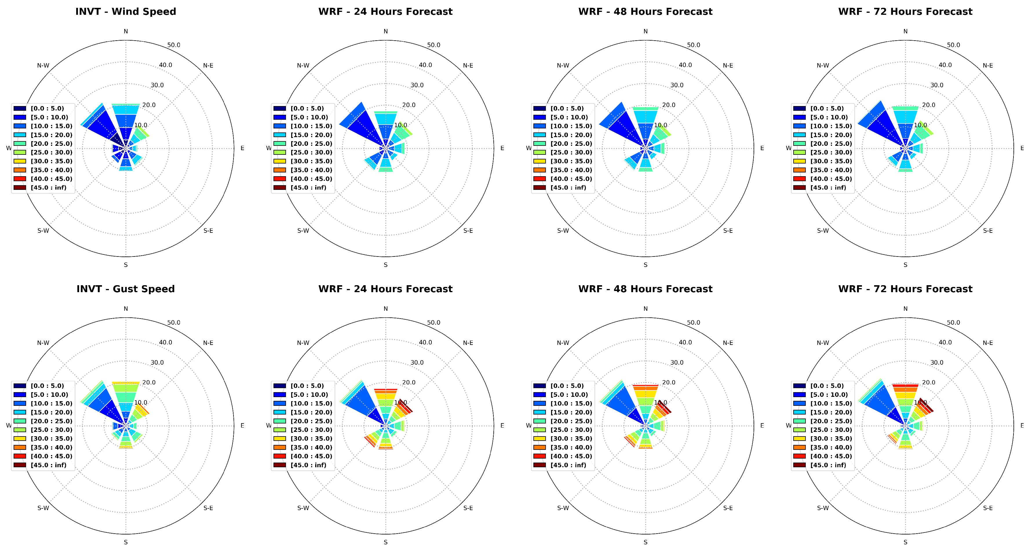
3.1. Assessing Model’s Performance during August 2021’s Event
3.2. Assessing Model’s Performance over a Year Long Simulation Period
4. Discussion and Conclusions
Author Contributions
Funding
Institutional Review Board Statement
Data Availability Statement
Acknowledgments
Conflicts of Interest
References
- Intergovernmental Panel on Climate Change (IPCC). Weather and Climate Extreme Events in a Changing Climate. In Climate Change 2021–The Physical Science Basis: Working Group I Contribution to the Sixth Assessment Report of the Intergovernmental Panel on Climate Change; Cambridge University Press: Cambridge, UK, 2023; pp. 1513–1766. [Google Scholar]
- Thomas, B.R.; Kent, E.C.; Swail, V.R.; Berry, D.I. Trends in ship wind speeds adjusted for observation method and height. Int. J. Climatol. 2008, 28, 747–763. [Google Scholar] [CrossRef]
- Tokinaga, H.; Xie, S.-P. Wave and Anemometer-Based Sea Surface Wind (WASWind) for Climate Change Analysis. J. Clim. 2011, 24, 267–285. [Google Scholar] [CrossRef]
- Young, I.R.; Zieger, S.; Babanin, A.V. Global Trends in Wind Speed and Wave Height. Science 2011, 332, 451–455. [Google Scholar] [CrossRef] [PubMed]
- Liu, Q.; Babanin, A.V.; Zieger, S.; Young, I.R.; Guan, C. Wind and Wave Climate in the Arctic Ocean as Observed by Altimeters. J. Clim. 2016, 29, 7957–7975. [Google Scholar] [CrossRef]
- Ribal, A.; Young, I.R. 33 years of globally calibrated wave height and wind speed data based on altimeter observations. Sci. Data 2019, 6, 77. [Google Scholar] [CrossRef]
- Andrade, K.M.; Pinheiro, H.R.; Neto, G.D. Extreme precipitation episode in Rio de Janeiro: Synoptic analysis, numerical simulation and comparison among previous events. Ciência Nat. 2015, 37, 175–180. [Google Scholar]
- Freitas, A.A.; Oda, P.S.S.; Teixeira, D.L.S.; Silva, P.N.; Mattos, E.V.; Bastos, I.R.P.; Nery, T.D.; Metodiev, D.; Santos, A.P.P.; Gonçalves, W.A. Meteorological conditions and social impacts associated with natural disaster landslides in the Baixada Santista region from March 2nd–3rd, 2020. Urban Clim. 2022, 42, 101–110. [Google Scholar] [CrossRef]
- Pereira Filho, A.J.; Pereira, J.D.; Vemado, F.; Silva, I.W. Operational Hydrometeorological Forecast System for Espírito Santo State, Brazil. J. Hydrol. Eng. 2015, 22, E5015003. [Google Scholar] [CrossRef]
- Souza, N.B.P.; Nascimento, E.G.S.; Moreira, D.M. Performance evaluation of the WRF model in a tropical region: Wind speed analysis at different sites. Atmósfera 2021, 36, 253–277. [Google Scholar] [CrossRef]
- Amarante, O.A.C.; Silva, F.J.L.; Andrade, P.E.P.; Parecy, E. Atlas Eólico: Espírito Santo; Agência de Serviços Públicos de Energia do Estado do Espírito Santo (ASPE): Vitória, Brazil, 2009. [Google Scholar]
- Oliveira, K.S.S.; Quaresma, V.S. Condições Típicas de Vento sobre a Região Marinha Adjacente à Costa do Espírito Santo. Rev. Bras. Climatol. 2018, 22, 503–523. [Google Scholar] [CrossRef]
- Skamarock, W.C.; Klemp, J.B.; Dudhia, J.; Gill, D.O.; Barker, D.; Duda, M.G.; Powers, J.G. A Description of the Advanced Research WRF Version 3; (NCAR/TN-475+STR); National Center for Atmospheric Research: Boulder, CO, USA, 2008. [Google Scholar]
- Skamarock, W.C.; Klemp, J.B.; Dudhia, J.; Gill, D.O.; Liu, Z.; Berner, J.; Wang, W.; Powers, J.G.; Duda, M.G.; Barker, D.M.; et al. A Description of the Advanced Research WRF Model Version 4.3; (NCAR/TN–556+STR); National Center for Atmospheric Research: Boulder, CO, USA, 2021. [Google Scholar]
- Skamarock, W.C.; Klemp, J.B.; Dudhia, J.; Gill, D.O.; Liu, Z.; Berner, J.; Wang, W.; Powers, J.G.; Duda, M.G.; Barker, D.M.; et al. A Description of the Advanced Research WRF Model Version 4; (NCAR/TN–556+STR); National Center for Atmospheric Research: Boulder, CO, USA, 2019. [Google Scholar]
- Tiedtke, M. A comprehensive mass flux scheme for cumulus parameterization in large-scale models. Mon. Weather Rev. 1989, 117, 1779–1800. [Google Scholar] [CrossRef]
- Thompson, G.; Field, P.R.; Rasmussen, R.M.; Hall, W.D. Explicit forecasts of winter precipitation using an improved bulk microphysics scheme. Part II: Implementation of a new snow parameterization. Mon. Weather Rev. 2008, 136, 5095–5115. [Google Scholar] [CrossRef]
- Janjic, Z. The step-mountain eta coordinate model: Further developments of the convection, viscous sublayer, and turbulence closure schemes. Mon. Weather Rev. 1994, 122, 927–945. [Google Scholar] [CrossRef]
- Tewari, M.; Chen, F.; Wang, W.; Dudhia, J.; Lemone, M.A.; Mitchell, K.E.; Ek, M.; Gayno, G.; Wegiel, J.W.; Cuenca, R. Implementation and verification of the unified NOAH land surface model in the WRF model. In Proceedings of the 20th Conference on Weather Analysis and Forecasting/16th Conference on Numerical Weather Prediction, American Meteorological Society, Seattle, WA, USA, 14 January 2004. [Google Scholar]
- Iacono, M.J.; Delamere, J.S.; Mlawer, E.J.; Shephard, M.W.; Clough, S.A.; Collins, W.D. Radiative forcing by long–lived greenhouse gases: Calculations with the AER radiative transfer models. J. Geophys. Res. 2008, 113, D13103. [Google Scholar] [CrossRef]
- Kain, J.S. The Kain–Fritsch convective parameterization: An update. J. Appl. Meteor. 2004, 43, 170–181. [Google Scholar] [CrossRef]
- Hong, S.-Y.; Dudhia, J.; Chen, S.-H. A revised approach to ice microphysical processes for the bulk parameterization of clouds and precipitation. Mon. Weather Rev. 2004, 132, 103–120. [Google Scholar] [CrossRef]
- Hong, S.-Y.; Noh, Y.; Dudhia, J. A new vertical diffusion package with an explicit treatment of entrainment processes. Mon. Weather Rev. 2006, 134, 2318–2341. [Google Scholar] [CrossRef]
- Jimenez, P.A.; Dudhia, J.; Gonzalez-Rouco, J.F.; Navarro, J.; Montavez, J.P.; Garcia-Bustamante, E. A revised scheme for the WRF surface layer formulation. Mon. Weather Rev. 2012, 140, 898–918. [Google Scholar] [CrossRef]
- Niu, G.-Y.; Yang, Z.-L.; Mitchell, K.E.; Chen, F.; Ek, M.B.; Barlage, M.; Kumar, A.; Manning, K.; Niyogi, D.; Rosero, E.; et al. The community Noah land surface model with multiparameterization options (Noah–MP): 1. Model description and evaluation with local–scale measurements. J. Geophys. Res. 2011, 116. [Google Scholar] [CrossRef]
- Rogers, E.; Black, T.; Ferrier, B.; Lin, Y.; Parrish, D.; DiMega, G. Changes to the NCEP Meso Eta Analysis and Forecast System: Increase in Resolution, New Cloud Microphysics, Modified Precipitation Assimilation, Modified 3DVAR Analysis. 2001. Available online: https://www.emc.ncep.noaa.gov/users/mesoimpldocs/mesoimpl/eta12tpb/ (accessed on 12 November 2023).
- Grell, G.A.; Devenyi, D. A generalized approach to parameterizing convection combining ensemble and data assimilation techniques. Geophys. Res. Lett. 2002, 29, 1693. [Google Scholar] [CrossRef]
- Chen, S.-H.; Sun, W.-Y. A one-dimensional time dependent cloud model. J. Meteor. Soc. Jpn. 2002, 80, 99–118. [Google Scholar] [CrossRef]
- Hong, S.-Y.; Lim, J.-O.J. The WRF single–moment 6–class microphysics scheme (WSM6). J. Korean Meteor. Soc. 2006, 42, 129–151. [Google Scholar]
- Grell, G.A. Prognostic Evaluation of Assumptions Used by Cumulus Parameterizations. Mon. Weather Rev. 1993, 121, 764–787. [Google Scholar] [CrossRef]
- Mlawer, E.J.; Taubman, S.J.; Brown, P.D.; Iacono, M.J.; Clough, S.A. Radiative transfer for inhomogeneous atmospheres: RRTM, a validated correlated–k model for the longwave. J. Geophys. Res. 1997, 102, 16663–16682. [Google Scholar] [CrossRef]
- Dudhia, J. Numerical study of convection observed during the Winter Monsoon Experiment using a mesoscale two–dimensional model. J. Atmos. Sci. 1989, 46, 3077–3107. [Google Scholar] [CrossRef]
- Nakanishi, M.; Niino, H. An improved Mellor–Yamada level 3 model: Its numerical stability and application to a regional prediction of advecting fog. Bound. Layer Meteor. 2006, 119, 397–407. [Google Scholar] [CrossRef]
- Ferreira, R.C.; Alves Junior, M.P.; Vendrasco, E.P.; Aravequia, J.A.; Nolasco Junior, L.R.; Biscaro, T.S. Impacto das Parametrizações de Microfísica na Previsão de Precipitação utilizando Assimilação de Dados de Radar. Rev. Bras. Meteorol. 2020, 35, 123–134. [Google Scholar] [CrossRef]
- Iacono, M.J. Application of Improved Radiation Modeling to General Circulation Models; Atmospheric and Environmental Research: Lexington, MA, USA, 2011. [Google Scholar]
- Pinto, L.I.C. Avaliação do Modelo WRF para Aplicação em Previsão de Recursos Eólicos no Nordeste Brasileiro. Ph.D. Thesis, National Institute for Space Research, São José dos Campos, Brazil, 2017. [Google Scholar]


| Grid 1 | Grid 2 | Grid 3 | |
|---|---|---|---|
| 9 km | 3 km | 1 km | |
| 65 | 79 | 55 | |
| 50 | 61 | 49 | |
| −22.68° | −21.22° | −20.50° | |
| −43.37° | −41.46° | −39.90° | |
| −18.02° | −19.37° | −20.08° | |
| −37.13° | −38.99° | −40.11° |
| Cumulus | MP | BL | SL | LS | LWR | SWR | |
|---|---|---|---|---|---|---|---|
| T1 | Tiedtke [16] | Thompson [17] | MYJ [18] | ETA [18] | Unified NOAH [19] | RRTMG [20] | RRTMG [20] |
| T2 | Kain-Fritsch [21] | WSM 3-class [22] | YSU [23] | MM5-REV [24] | NOAH-MP [25] | RRTMG [20] | RRTMG [20] |
| T3 | Kain-Fritsch [21] | Ferrier [26] | YSU [23] | MM5-REV [24] | NOAH-MP [25] | RRTMG [20] | RRTMG [20] |
| T4 | Grell-Devenyi [27] | Ferrier [26] | YSU [23] | MM5-REV [24] | NOAH-MP [25] | RRTMG [20] | RRTMG [20] |
| T5 | Kain-Fritsch [21] | Purdue Lin [28] | YSU [23] | MM5-REV [24] | NOAH-MP [25] | RRTMG [20] | RRTMG [20] |
| T6 | Tiedtke [16] | WSM 6-class [29] | YSU [23] | MM5-REV [24] | NOAH-MP [25] | RRTMG [20] | RRTMG [20] |
| T7 | Grell 3D [30] | WSM 3-class [22] | YSU [23] | MM5-REV [24] | NOAH-MP [25] | RRTM [31] | Dudhia [32] |
| T8 | Kain-Fritsch [21] | Purdue Lin [28] | MY-NN3 [33] | MM5-REV [24] | NOAH-MP [25] | RRTMG [20] | RRTMG [20] |
| T9 | Kain-Fritsch [21] | Ferrier [26] | MY-NN3 [33] | MM5-REV [24] | NOAH-MP [25] | RRTMG [20] | RRTMG [20] |
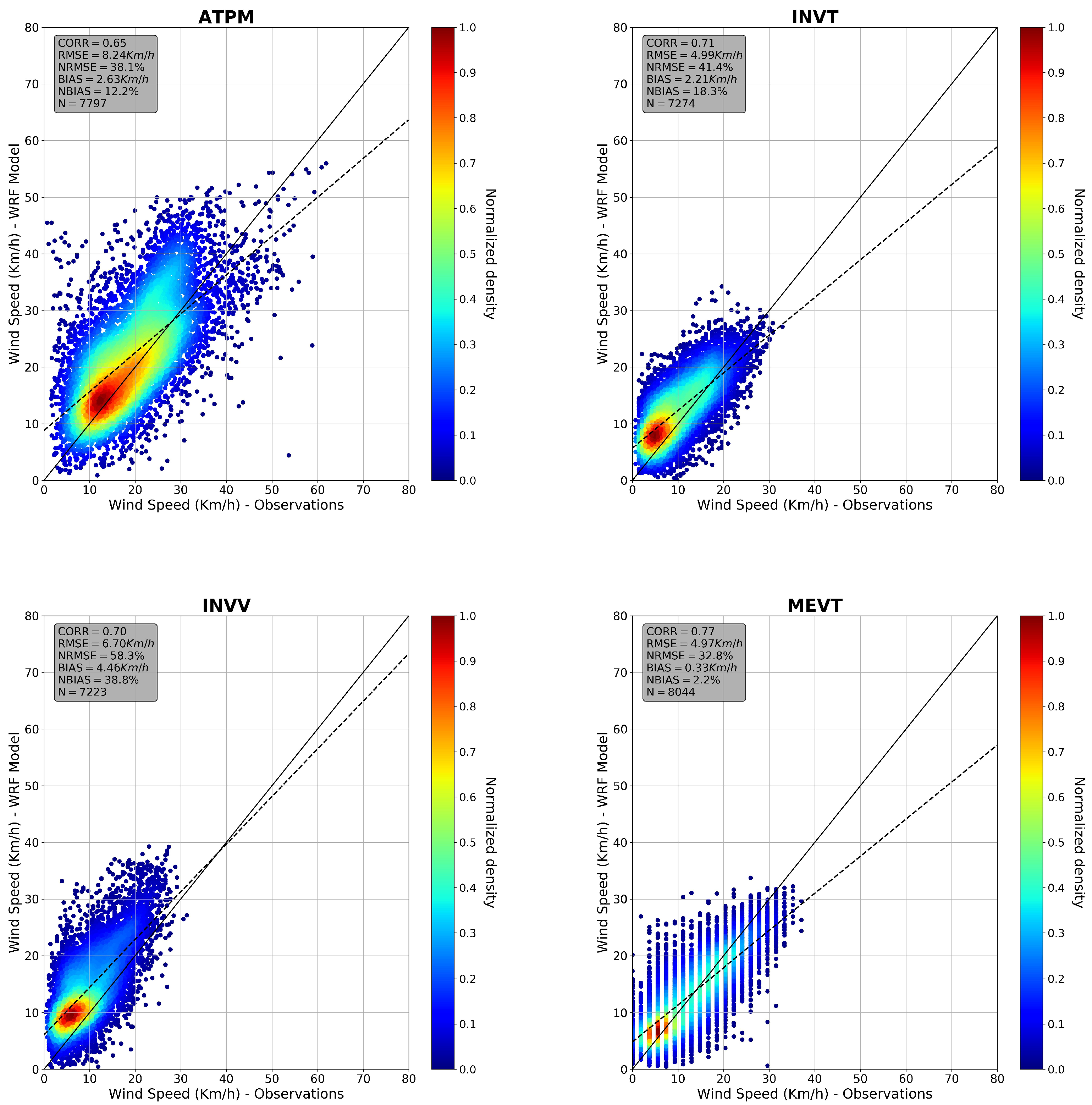
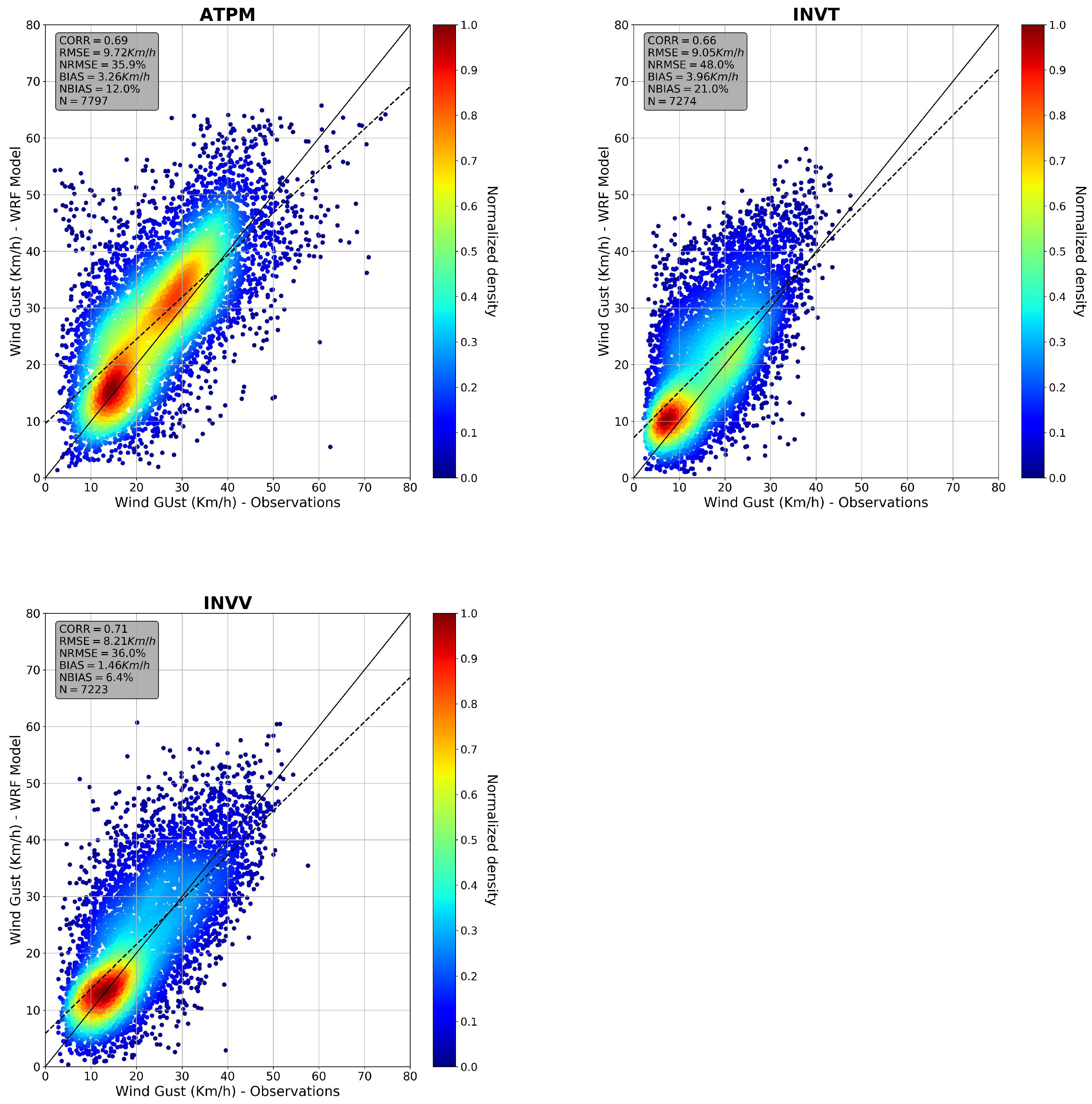
| CORR | BIAS | NBIAS | RMSE | NRMSE | SI | ||
|---|---|---|---|---|---|---|---|
| (km/h) | (%) | (km/h) | (%) | (%) | |||
| ATPM | Wspd-24 h | 0.65 | 2.63 | 12.20 | 8.24 | 38.1 | 40.67 |
| Gust-24 h | 0.69 | 3.26 | 12.00 | 9.72 | 35.90 | 37.94 | |
| Wspd-48 h | 0.62 | 2.71 | 12.40 | 8.61 | 39.6 | 43.26 | |
| Gust-48 h | 0.64 | 3.63 | 13.30 | 10.56 | 38.80 | 41.85 | |
| Wspd-72 h | 0.60 | 2.47 | 11.30 | 8.71 | 40,0 | 43.88 | |
| Gust-72 h | 0.62 | 3.40 | 15.50 | 10.78 | 39.50 | 42.85 | |
| INVT | Wspd-24 h | 0.71 | 2.21 | 18.30 | 4.99 | 41.4 | 42.9 |
| Gust-24 h | 0.66 | 3.96 | 21.00 | 9.05 | 48.00 | 38.5 | |
| Wspd-48 h | 0.69 | 2.41 | 20.00 | 5.20 | 43.10 | 46.00 | |
| Gust-48 h | 0.64 | 4.30 | 22.80 | 9.41 | 49.90 | 39.90 | |
| Wspd-72 h | 0.69 | 2.31 | 19.20 | 5.18 | 43.00 | 46.20 | |
| Gust-72 h | 0.63 | 4.10 | 21.70 | 9.46 | 50.1 | 40.20 | |
| INVV | Wspd-24 h | 0.70 | 4.46 | 38.80 | 6.70 | 58.30 | 49.90 |
| Gust-24 h | 0.71 | 1.46 | 6.40 | 8.21 | 36.00 | 39.40 | |
| Wspd-48 h | 0.67 | 4.66 | 40.60 | 7.03 | 61.2 | 54.10 | |
| Gust-48 h | 0.68 | 1.78 | 7.80 | 8.85 | 38.80 | 39.50 | |
| Wspd-72 h | 0.66 | 4.66 | 40.70 | 7.07 | 61.70 | 54.80 | |
| Gust-72 h | 0.66 | 1.76 | 7.70 | 9.12 | 40.10 | 44.80 | |
| MEVT | Wspd-24 h | 0.77 | 0.33 | 2.20 | 4.97 | 32.80 | 38.10 |
| Wspd-48 h | 0.74 | 0.57 | 3.80 | 5.32 | 35.10 | 42.00 | |
| Wspd-72 h | 0.74 | 0.57 | 2.70 | 5.35 | 35.30 | 42.30 |
Disclaimer/Publisher’s Note: The statements, opinions and data contained in all publications are solely those of the individual author(s) and contributor(s) and not of MDPI and/or the editor(s). MDPI and/or the editor(s) disclaim responsibility for any injury to people or property resulting from any ideas, methods, instructions or products referred to in the content. |
© 2024 by the authors. Licensee MDPI, Basel, Switzerland. This article is an open access article distributed under the terms and conditions of the Creative Commons Attribution (CC BY) license (https://creativecommons.org/licenses/by/4.0/).
Share and Cite
Gonçalves, L.d.J.M.; Kaiser, J.; Palmeira, R.M.d.J.; Gallo, M.N.; Parente, C.E. Evaluation of a High Resolution WRF Model for Southeast Brazilian Coast: The Importance of Physical Parameterization to Wind Representation. Atmosphere 2024, 15, 533. https://doi.org/10.3390/atmos15050533
Gonçalves LdJM, Kaiser J, Palmeira RMdJ, Gallo MN, Parente CE. Evaluation of a High Resolution WRF Model for Southeast Brazilian Coast: The Importance of Physical Parameterization to Wind Representation. Atmosphere. 2024; 15(5):533. https://doi.org/10.3390/atmos15050533
Chicago/Turabian StyleGonçalves, Layrson de Jesus Menezes, Júlia Kaiser, Ronaldo Maia de Jesus Palmeira, Marcos Nicolás Gallo, and Carlos Eduardo Parente. 2024. "Evaluation of a High Resolution WRF Model for Southeast Brazilian Coast: The Importance of Physical Parameterization to Wind Representation" Atmosphere 15, no. 5: 533. https://doi.org/10.3390/atmos15050533