Article

Importance of Ship Emissions to Local Summertime Ozone Production in the Mediterranean Marine Boundary Layer: A Modeling Study

by
Christian N. Gencarelli
1,
Ian M. Hedgecock
1,*,
Francesca Sprovieri
1,
Gregor J. Schürmann
1,† and
Nicola Pirrone
2
1
Division of Rende, CNR-Institute of Atmospheric Pollution Research, Rende 87036, Italy
2
CNR-Institute of Atmospheric Pollution Research, via Salaria km 29,300, Monterotondo 00015, Italy
*
Author to whom correspondence should be addressed.
Current Address: Biogeochemical Systems Department, Max Planck Institute for Biogeochemistry, Postfach 10 01 64, Hans-Knöll-Str. 10, Jena 07745, Germany
Atmosphere 2014, 5(4), 937-958; https://doi.org/10.3390/atmos5040937
Submission received: 22 September 2014 / Revised: 24 October 2014 / Accepted: 11 November 2014 / Published: 2 December 2014

Abstract

:
Ozone concentrations in the Mediterranean area regularly exceed the maximum levels set by the EU Air Quality Directive, 2008/50/CE, a maximum 8-h mean of 120 µg·m−3, in the summer, with consequences for both human health and agriculture. There are a number of reasons for this: the particular geographical and meteorological conditions in the Mediterranean play a part, as do anthropogenic ozone precursor emissions from around the Mediterranean and continental Europe. Ozone concentrations measured on-board the Italian Research Council’s R. V. Urania during summer oceanographic campaigns between 2000 and 2010 regularly exceeded 60 ppb, even at night.  The WRF/Chem (Weather Research and Forecasting (WRF) model coupled with Chemistry) model has been used to simulate tropospheric chemistry during the periods of the measurement campaigns, and then, the same simulations were repeated, excluding the contribution of maritime traffic in the Mediterranean to the anthropogenic emissions inventory. The differences in the model output suggest that, in large parts of the coastal zone of the Mediterranean, ship emissions contribute to 3 and 12 ppb to ground level daily average ozone concentrations. Near busy shipping lanes, up to 40 ppb differences in the hourly average ozone concentrations were found. It seems that ship emissions could be a significant factor in the exceedance of the EU directive on air quality in large areas of the Mediterranean Basin.

1. Introduction

The Mediterranean Basin has a number of characteristics that favor boundary layer (BL) ozone formation, especially in the summer. During the summer, the Mediterranean is under the descending arm of the Hadley circulation and, therefore, enjoys long periods of anticyclonic weather, with high temperatures and intense sunshine. These conditions favor both O3 formation and the natural production of VOC [1]. The presence of major urban and industrial centers on the coasts and the general north to south BL flow [2] mean that anthropogenic O3 precursors are abundant.
Elevated concentrations of O3 have been observed at inland sites [3], coastal sites [4,5,6] and during intensive field campaigns [2]. Measurements over the sea, performed on-board a cruise liner over two summers [7] and on-board the Italian Research Council’s R. V. Urania (as described here) also found high O3 concentrations. Local circulation patterns also enhance O3 levels. The often steep coastal orography, particularly in the Western Basin, produces local circulation patterns, which carry polluted coastal air over the sea at night, where it remains until morning, when the breeze off the sea carries it back over land [1,7,8,9]. In the Eastern Mediterranean Basin, increasing urbanization is leading to the creation of mega-cities, such as Istanbul and Cairo, which are having an impact on regional air quality [10,11].
Ozone produced in the boundary layer can be advected upwards to the free troposphere. For example, in Italy, polluted air from the Po Valley has regularly been detected on Monte Cimone, in the Apennines [3,12,13]. Increasing O3 concentrations in the free troposphere over the Mediterranean is of concern, because its effect as a greenhouse gas is greater in the free troposphere than it is in the boundary layer; generally speaking, the capacity of O3 to trap heat in the atmosphere increases from the ground to the tropopause [14]. Furthermore, recently, Richards et al. [15] showed that ozone formation in the lower troposphere was significantly influenced by local NOx and VOC emission. Another factor that may begin to contribute to O3 production in the region is increasing temperatures [16]; a recent study by Im and Kanakidou [11] estimated that for each 1 K rise in temperature, average O3 concentrations would increase by 1 ppb.
The Mediterranean has a number of major ports and, because of the presence of the entrance to the Suez Canal, is also a major thoroughfare for international maritime traffic. Emissions from shipping have come under scrutiny in recent years, particularly because of the influence their SOx, NOx and particulate matter can have on air quality in coastal areas and port towns [17,18,19,20,21,22,23,24,25]. Abundant emissions from shipping can also lead to acidification and eutrophication, via nitrate deposition to coastal waters and land [26,27]. This study however focuses specifically on the impact of ship emissions on summertime O3 concentrations and covers a longer period than most previous studies, which have concentrated on shorter periods or specific campaigns.
Maps of emissions over the Mediterranean Sea (see Figure S1) show quite clearly the major routes used by maritime traffic, with high densities between Gibraltar and the entrance to the Suez canal, in the Adriatic, around the ports of southern France and eastern Spain and through the Aegean to the Dardanelles and Bosphorus.
The influence of shipping emissions on air quality in the Mediterranean is likely to increase as global maritime traffic increases. Furthermore, as legislation regarding industry and transport on land continues to curtail emissions from these sources, the relative importance of emissions from ships will increase.
The Italian Research Council’s R. V. Urania has undertaken a series of summer oceanographic campaigns to study the Hg cycle in the Mediterranean beginning in the summer of 2000. During these campaigns, O3 concentrations were measured continuously. The campaign in 2005 was mostly performed in the Adriatic, and it was noted that the average O3 concentration for the whole period was just over 60 ppb (including nighttime values) [28]. This prompted this investigation into one of the possible causes of high O3 levels over the Mediterranean.
The WRF/Chem(Weather Research and Forecasting (WRF) model coupled with Chemistry) model [29] has been used to simulate atmospheric composition over the periods of six of these campaigns between 2000 and 2010, using the EMEP (European Monitoring and Evaluation Programme) emissions database. The data from the campaigns has been used to ascertain the reliability of the model output, and the WRF/Chem simulations have been rerun excluding the emissions from shipping in the anthropogenic emission inventory. Comparison of the results of the two simulations gives insight into the scale of the impact that Mediterranean maritime traffic has on O3 concentrations in the region.

2. Measurements

Measurements from six oceanographic campaigns and from EMEP network monitoring stations have been used for comparison with the modeled O3 concentrations. From 2000, an almost yearly series of oceanographic campaigns, primarily to study Hg cycling in the Mediterranean marine BL (MBL), surface and column water, sediments and the exchange of Hg species between the atmosphere and the sea surface have been performed aboard the R. V. Urania by the CNR-IIA (Italain Research Council Institute of Atmospheric Pollution Research) [30,31,32,33,34]. In addition to Hg species, a number of gas and aerosol phase atmospheric species were measured. The campaign periods, their start and end ports, are summarized with a brief description of the area covered in Table 1. The routes are shown in Figure 1. During the campaigns, ozone concentrations were measured using a Teledyne-API model 400A UV ozone analyzer. The analyzer was calibrated every 24 h using an internal permeation source, and employing a sampling flow rate of 0.8 l min−1 over a five-minute period gave a detection limit of 0.6 ppb. The same instrument was used in all measurement campaigns.
The EMEP monitoring station data used for comparison with model output were located in the middle resolution modeling domain, the position of which varied according to the campaign route taken in the year in question; see Section 3.1. The stations used are shown in Figure 1 and listed in Table S1 (see Hjellbrekke et al. [35] for details).
Table 1. The oceanographic campaign periods and approximate routes.
YearStartEndRoute
2000Palermo 14 JulyCivitavecchia 9 AugustStrait of Messina, South of Crete, Sicily, Gulf of Naples, Sardinia
2003Palermo 5 AugustLivorno 28 AugustStrait of Sicily, towards Crete, Ionian Sea, Naples, Alboran Sea
2005Naples 17 JuneNaples 3 JulySicily, Ionian Sea, Adriatic Sea
Gulf of Trieste
2006Civitavecchia 4 JulyMessina 20 JulySicily, Eastern Mediterranean, Ionian Sea
2009Civitavecchia 4 JuneMessina 30 JuneCorsica, Sardinia, Naples, Strait of Sicily, Ionian Sea
2010Naples 27 AugustPalermo 12 SeptemberPalermo Strait of Messina, Ionian sea, Gulf of Taranto, Eastern Mediterranean, Strait of Sicily
Figure 1. The Med-Oceanor campaign routes over the years and the sites of the European Monitoring and Evaluation Programme (EMEP) stations used in the model validation.
Atmosphere 05 00937 g001

3. Modeling

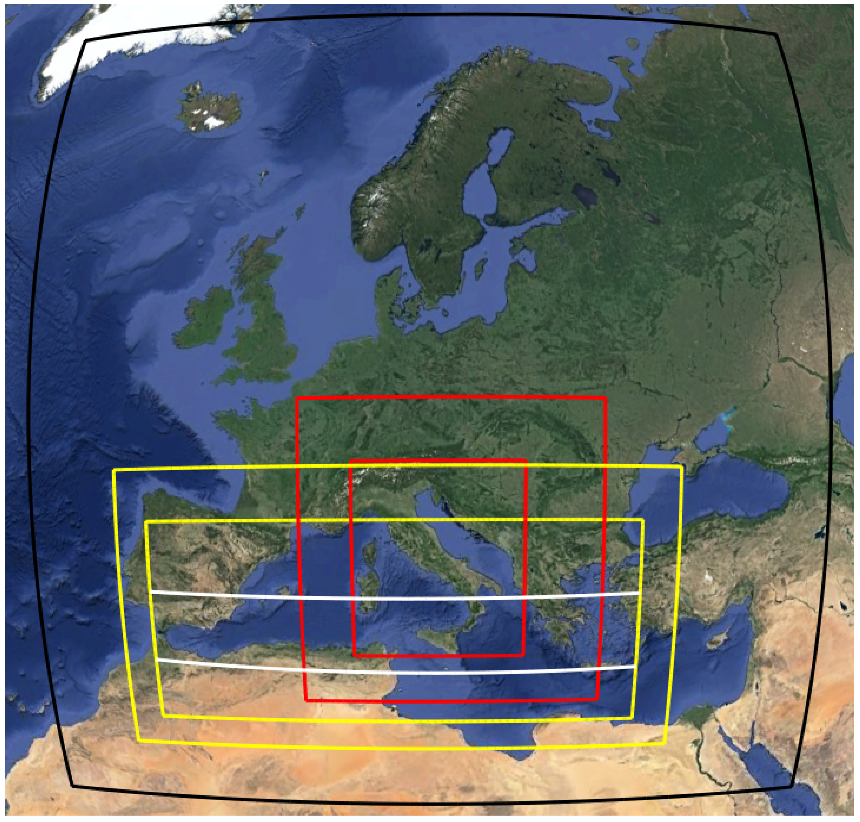
3.1. Modeling Domains

Three model domains were used to model each oceanographic campaign period. The largest domain (81 × 81 km grid cells) remained the same in all of the simulations. The finest scale domain (9 × 9 km grid cells) was chosen to include the area covered by the oceanographic campaign, and the intermediate domain (27 × 27 km grid cells) was chosen to encompass the fine domain and to provide a buffer between the coarse and fine domains. The coarse domain and two examples of the nested domains are shown in Figure 2, while all model domains are shown in Figures S2–S6. The domains extended vertically to 50 hPa with 28 levels.
Figure 2. The largest modeling domain (black) and examples of the nested grids, for 2003 in yellow and for 2005 in red, displayed in GoogleTM Earth. The two horizontal white lines in the smallest 2003 domain are the cross-sections at roughly 34 and 39° N described in Section 4.4. See Figures S2–S6 for all model domains.
Atmosphere 05 00937 g002

3.2. Physics, Chemistry and Initialization

The non-hydrostatic mesoscale chemical transport model, WRF/Chem, offers a number of parametrization options to represent atmospheric physics (a detailed description of these can be found in Skamarock et al. [36]). In this study, the Purdue–Lin scheme, which includes six classes of hydrometeors (cloud water and ice, rain, snow, graupel and water vapor) was used for microphysics. The Mellor–Yamada–Janjic (MYJ) scheme was used for Planetary Boundary Layer (PBL) parametrization; this scheme describes vertical sub-grid-scale fluxes due to eddy transport in the whole atmospheric column, while the horizontal eddy diffusivity is calculated with a Smagorinsky first order closure. The Eta surface layer scheme and the Noah land surface model (four soil layers) were used. The Kain–Fritsch scheme was used for cumulus parametrization and the rapid radiative transfer model (RRTM) and Dudhia schemes for long and shortwave radiation, respectively.
The choice of parametrizations was made after repeated simulations of the 2005 oceanographic campaign period using different combinations of parametrizations, to assess how the choice influenced both model output and simulation time. The combination used proved to be the most appropriate for these studies. However, it should be pointed out that the simulations performed apply specifically to the Mediterranean summer and that the combination of parametrizations above may not be the most appropriate in other cases.
The RADM2 (Regional Acid Deposition Model, version 2) mechanism [37] and the Madronich photolysis scheme [38] were used in all of the simulations. Photolysis rate constants were recalculated every 30 min.
NCEP FNL (final) Global Operational Analyses, obtained from the Research Data Archive (RDA), provided on a 1° by 1° grid at six hourly intervals, were used to provide meteorological input data. The data are converted to WRF input on the appropriate domains using the WRF Preprocessing System (WPS). Boundary and initial conditions for chemical species concentrations for the largest domain were taken from the idealized profile provided by WRF/Chem. The model was allowed to spin-up for five days before the beginning of the observation period under study.

3.3. Emissions

Anthropogenic emissions were obtained from the EMEP Centre for Emission Inventories and Projections [39]. The emissions used in EMEP models [40] for the specific years corresponding to the measurement campaigns were used. As in Schürmann et al. [41], a day-night temporal profile was applied to the emissions following Simpson et al. [42].
The EMEP emissions were chosen because of their specificity to the European region, their availability for individual years and also the results obtained by Marmer et al. [43] in a comparison of shipping emission inventories for the Mediterranean Sea. Marmer et al. [43] found that in their modeling study, the EMEP inventory gave the best match with the major part of the measurements with which they compared their simulations, particularly in the Western Basin.
The online option to estimate biogenic emissions using the approach described by Guenther et al. [44,45] and Simpson et al. [46] was used. The alternative option using the biogenic emission fluxes calculated using MEGAN (Model of Emissions of Gases and Aerosols from Nature) [47] was also used for the 2005 campaign simulations.

3.4. In-Plume Chemistry and Artificial Plume Dilution

The perturbation caused by ship emissions to BL photochemistry over oceans began to be investigated in detail in the late 1990s [48,49]. The direct inclusion of ship emissions in Chemical Transport Models (CTMs)will result in the instantaneous dilution of the emissions within the volume of the grid cell. In coarse resolution models, this leads to a false impression of the chemical composition in the model cell, because the chemistry occurring within the expanding plume, where the chemical composition is different from the air in the rest of the cell, is not taken into account (see Charlton-Perez et al. [50], Huszar et al. [51] and Vinken et al. [52]). This can lead to errors in the simulation of NOx and OH concentrations and in the simulated ozone production efficiency [50] and, over the open sea, leads to an overestimate of the O3 concentration.
However, a GEOS-Chem model study of the effect of including non-linear chemistry for ship emissions [52] indicates that the impact of dilution is less significant over more heavily polluted areas, such as the North Sea; the authors state “suggesting that accounting for non-linear in-plume chemistry is most relevant for pristine, unpolluted areas”.
Ship plume dilution also depends on a the combination of BL stability, the plume’s buoyancy (it is hotter than the surrounding air) and the ship’s course relative to the wind speed and direction [53]. These factors influence both plume rise, which can be 2–10-times the actual stack height, and the shape of the plume (see Chosson et al. [53] and the references therein).
The simulations described here all concern the Mediterranean Basin. The Mediterranean BL is influenced by many other emission sources besides shipping, and during the summertime, when the oceanographic cruises took place, BL outflow from continental Europe is a major source of anthropogenic emissions to the region [2]. Therefore, considering the non-pristine’ state of the Mediterranean BL, the emissions were interpolated directly into the modeling domain, and sub-grid scale parametrizations were not used. However, two emission height scenarios were used to investigate the possible effects of plume rise; see Section 3.5.

3.5. The Simulations Performed

The introduction of the emissions into the modeling domain mirrors the approach used by Huszar et al. [51], where the emissions from the EMEP database were interpolated directly on to the model grid. Two emission height cases were investigated for the shipping emissions to ascertain how much emission injection height influenced the simulation results. In the EMEP unified model, all emissions from SNAP (Selected Nomenclature for Air Pollution) Sector 8 (other mobile sources and machinery, which includes shipping) are assumed to be emitted in the first model layer (0–92 m). The WRF/Chem simulations described here, given the synoptic conditions prevailing during the periods investigated, generally had five vertical levels from sea level to roughly 400 m a.s.l. over the open Mediterranean. This is a fairly typical height of the Mediterranean BL under summertime anticyclonic conditions. Two emission height scenarios have been used: the Em_low scenario, where the emissions are emitted into the first model level, and the Em_hi scenario, where the emissions are distributed between Levels 2 (≈30–90 m, 50%), 3 (≈90–160 m, 25%) and 4 (≈160–250 m, 25%).

4. Results and Discussion

4.1. Model Validation

Model results have been compared to the O3 data obtained during the oceanographic campaigns. The mean bias (MB), correlation coefficient (R), root mean square error (RMSE) and index of agreement (IOA) were used to assess the comparison, as defined in Chang and Hanna [54] and Willmott et al. [55]. Using the relation RMSE2 = RMSE u 2 + RMSE s 2 [55], the unsystematic fraction of RMSE (UF) is defined as:
UF = RMSE u 2 RMSE 2
The UF provides an estimate of the percentage of the RMSE not due to systematic errors.
Comparison with measurements from land-based monitoring sites was performed for the sites that were within the middle domain (27 km by 27 km resolution). For these measurements, similarly to Zhang et al. [56] (based on US-EPA guidelines [57]) the mean normalized bias (MNB), normalized gross error (NGE) and the accuracy of the unpaired predicted to observed peak hourly O3 concentration ratio (AUP) have been calculated.
The skill of the WRF/Chem model using the RADM2 mechanism in reproducing meteorological and air quality parameters has been assessed in a number of previous studies [29,41,58,59,60,61]; thus, the principal aim of this study is to assess the impact of shipping emissions on O3 concentrations, and therefore, the priority was to test the model’s performance in reproducing measured O3.

4.2. Ozone Concentration Validations

A number of studies of ozone using WRF/Chem have recently been performed. For example, for regions in the U.S. [29,60,62,63,64,65], Mexico City [58,66], for regions in Europe [41,59,67] and in China [61].
The summary of the statistical measures to assess the model’s performance in reproducing the observations during the oceanographic measurement campaigns is presented in Table 2. The agreement between the modeled concentrations and the observations are on par with those from previous studies.
Table 2. Comparison of the hourly model results and the ozone concentrations measured aboard the R. V. Urania; see Section 3.3 for the definition of the Em_low and Em_hi emission scenarios. The results for 2003 consider only the first half of the campaign; see Section 4.2. MB, mean bias; IOA, index of agreement; UF, unsystematic fraction.
YearMB (ppb)RRMSE (ppb)UFIOA
lowhilowhilowhilowhilowhi
2000−3.70.70.510.5911.09.60.590.680.690.76
20034.03.70.320.3114.714.70.470.480.550.54
20053.04.60.550.5613.813.50.800.690.730.72
20069.9−8.80.240.1914.514.30.330.400.480.49
20097.87.90.300.2914.915.30.550.560.530.52
2010−0.7−1.20.390.3810.710.90.730.730.630.63
Table 2 includes the results from the two emission height scenarios (Em_hi and Em_low) mentioned in Section 3.4. The differences between these are discussed further below (see Section 4.3); however, as can be seen from Table 2, the difference in the results in the first model layer are not very large. The model does not consistently over- or under-estimate the ozone concentrations; the bias in some years is negative and others positive. Generally the model reproduces the measured O3 concentrations reasonably well; furthermore, the UF value does not show evidence of significant systematic errors.
Figure 3 shows the modeled and measured O3 concentrations for the oceanographic campaigns. The rapid decreases in O3 seen in the measurements occur when the R.V. Urania is directly influenced by plumes from ships passing close by or when the ship is stationary to take water column and sediment samples, and the wind direction carries the ships own exhaust towards the O3 analyzer. When this occurs, the high levels of NO decrease the O3 concentration, forming NO2. This titration effect means that the correlation between the daily minimum observed and modeled O3 concentrations was generally poor. The modeled and measured maximum daily values were better correlated, as were the daily mean values, with values of R over 0.6 in some cases (Table S2).
Figure 3. Measured and modeled O3 concentration ( ppb) during the oceanographic campaigns (model values from the Em_hi scenario).
Atmosphere 05 00937 g003
Some technical difficulties with the data collection occurred for short periods during the campaigns in 2000 (from 28 July to 6 August) and 2003 (around 18 August). These periods have been excluded from the observation/model comparison. The direct influence of other ships on O3 concentrations was particularly clear during the second period of the 2003 campaign (from 19 to 27 August, Naples -the Strait of Gibraltar-Livorno) when some of the lowest O3 concentrations recorded during any of the Med-Oceanor campaigns were measured, below 20 ppb at times. The mean observed O3 concentrations for the first (5–16 August) and second periods are 65.6 ppb and 50.4 ppb respectively; such a difference is not evident in any of the other Med-Oceanor campaigns. The metrics reported in Table 2 refer to the first eleven days of the 2003 campaign.
The model comparison with the land-based measurement stations gave results essentially similar to the comparison with the MBL measurements. The results of the comparison are reported in Table S3 and Figures S7–S12 and summarized in Figure 4. Generally, the model reproduces the land-based measurements according to the criteria set out in Zhang et al. [56] (±15% for MNB, <35% for NGE and ±20% for AUP). The model slightly underestimates peak O3 concentrations in a number of stations, particularly for the 2009 simulation.
Figure 4. Statistical metrics of hourly ozone concentration in the EMEP sites in the different simulations. The right-hand panels represent all data.
Atmosphere 05 00937 g004
The comparison between the modeled and measured O3 concentrations also reveals that the model does not reproduce the amplitude of the day-night variation in concentration well. This is very possibly due to difficulties in accurately modeling the temporal evolution of the boundary layer. If the nighttime boundary layer is too high in the model, both the rate at which O3 is deposited, and the rate at which it is titrated by species emitted at the surface would be underestimated. The daytime underestimate of the O3 maximum may also be ascribed to the model’s failure to correctly represent boundary layer dynamics, as the mixing down of O3 rich air plays an important role in the increase of the daytime O3 concentration.

4.3. The Influence of Ship Emission Height in the Model

As described in Section 3.3, two shipping emission injection height scenarios have been studied with the model. The first, the Em_low scenario, simply introduces ship emissions into the first model layer, while the Em_hi scenario distributes emissions between the second, third and fourth model layers (that is, between 30 and 250 m) to estimate the possible changes in model output accounting for plume rise (see Section 3.3). The results in Table 2 show that the comparison between the modeled and measured O3 concentrations in both instances is very similar. The difference between the emission height scenarios is most clearly seen in the first model layer, whereas the difference in the scenarios over the first six model layers (roughly the height of the Mediterranean summertime MBL) is actually only a few percent for O3, NO or NO2. The differences in the average concentrations over the highest resolution domain (9 km by 9 km) and over the whole simulation period is shown as a percentage in Figure 5 for 2005 and 2009, calculated as:
| [ X Em_hi ] [ X Em_low ] 1 | × 100
where X is O3, NO or NO2 (note the modulo). The results for the other campaigns are included in Figure S13. As can be seen, the difference between the emission scenarios is more marked in the first model layer, especially for NOx concentrations, while it is rarely more than 5% over the full height of the MBL. The exception to this is the simulations for the year 2000, where the difference between the simulations reaches almost 5% for O3 and almost 10% for NO2.
Figure 5. Concentration difference (calculated as Equation (2)) for O3, NO and NO2 in the first model layer and in the Mediterranean boundary layer (MBL).
Atmosphere 05 00937 g005

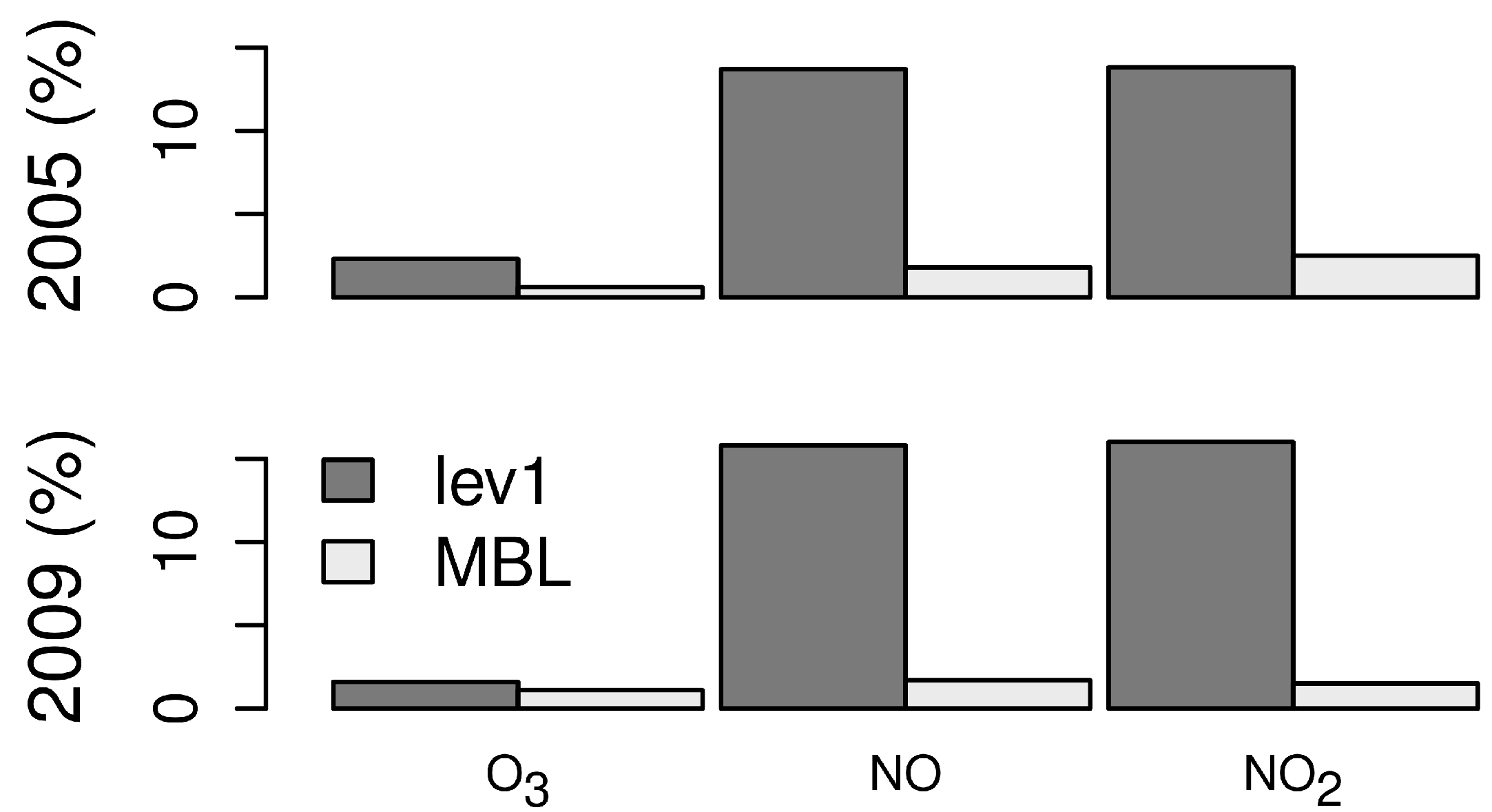
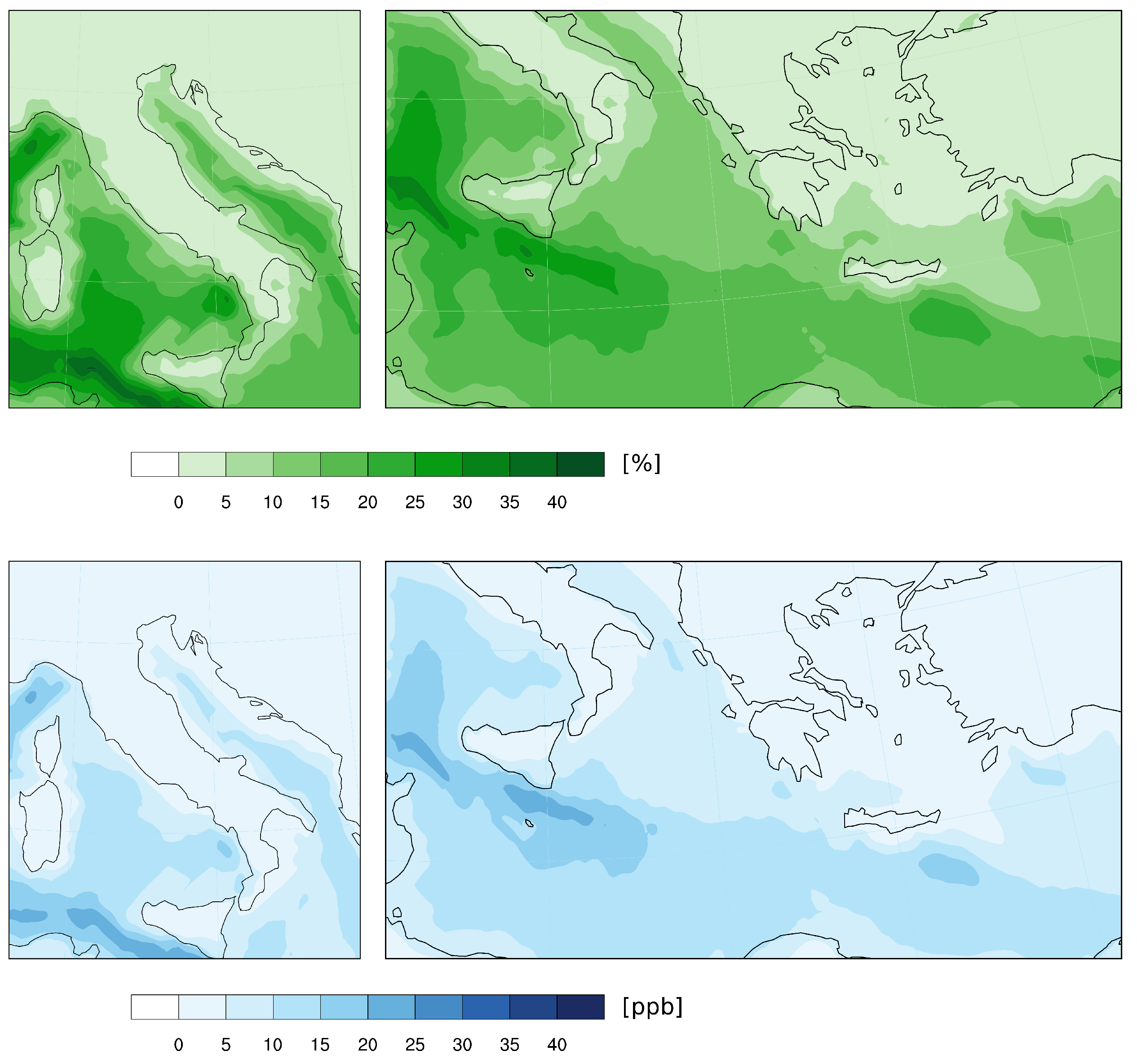
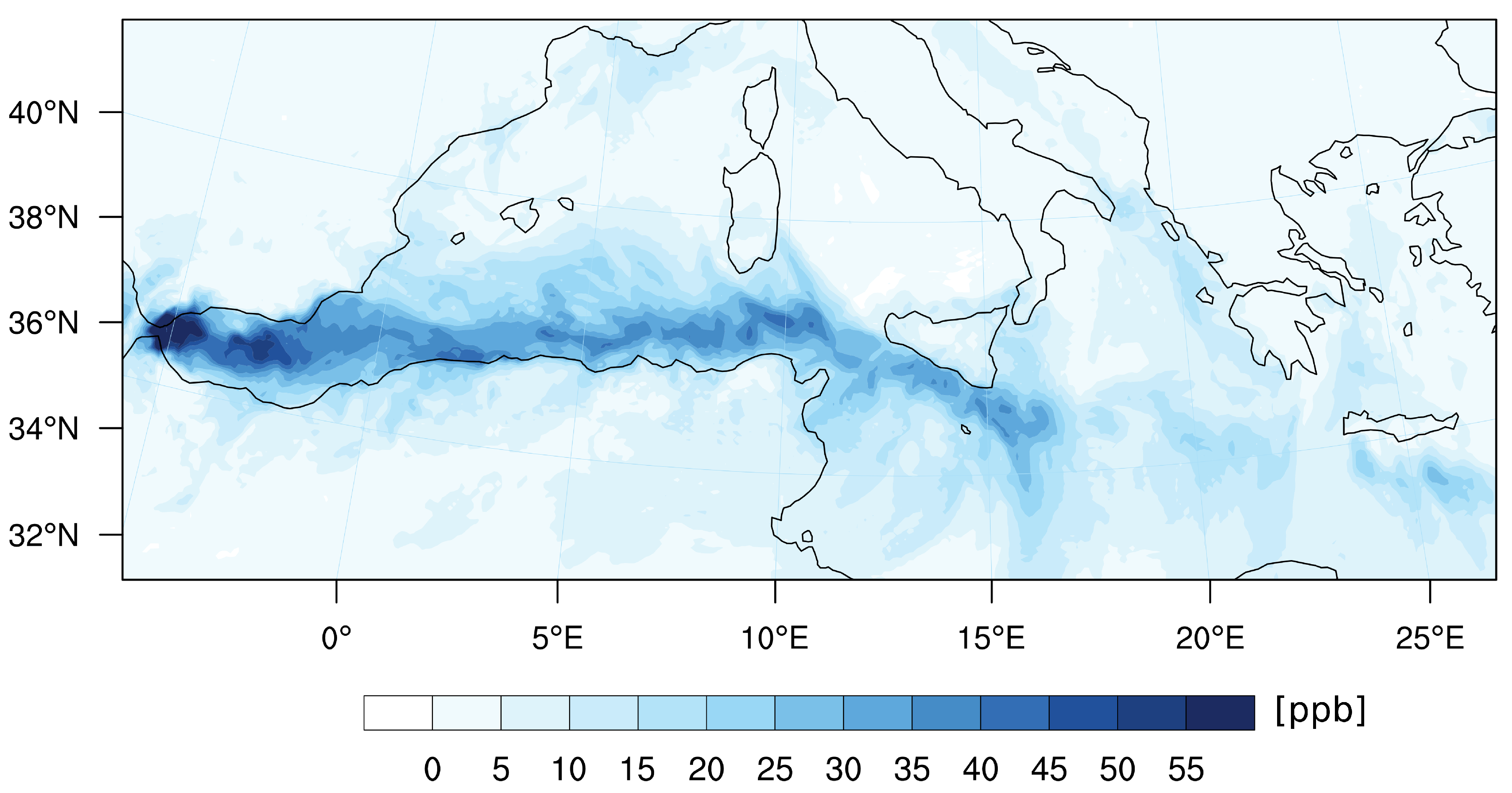
4.4. The Influence of Ship Emissions

Versions of the EMEP emission inventory for the years of oceanographic campaigns were prepared in which all of the SNAP sector 8 emissions over the Mediterranean Sea were removed.
The Em_Hi scenario simulations described previously were rerun, for exactly the same periods and on exactly the same domains. An overview of the results is presented in Table 3 where the difference (in %) between the concentrations of O3, NO and NO2 for simulations with (Tot_Emiss) and without (No_ships) shipping emissions are shown.
Table 3. The influence (%) of shipping emissions on the average concentrations of O3, NO and NO2 in the first six layers. The values refer to the highest resolution domains (9 km by 9 km), calculated as (Tot_Emiss − No_Ships)/Tot_Emiss × 100%.
YearWhole DomainMediterranean Sea
O3NONO2O3NONO2
20005.511.211.96.220.023.2
20037.010.311.08.224.928.9
20054.56.97.48.225.027.7
20065.312.213.18.326.930.9
20099.120.221.811.642.646.0
20107.715.913.89.830.132.7
Roughly speaking, removing the emissions from ships results in a decrease in the modeled average O3 concentration over the whole of the highest resolution domains (9 km by 9 km) of between 4.5% and 9.1%. The decrease over the Mediterranean Sea itself was between 6.2% and 11.6% for the periods simulated. These values are significant given the size of the domain and the lengths of time involved; however, the effect of shipping emissions is clearly not uniform over the whole domain.
While Table 3 gives the average differences over the whole domain (and just the Mediterranean), Figure 6 shows the simulated time averaged impact of shipping emissions for 2005 (left) and 2006 (right). Figures for the other years are included in the supplementary file (Figures S14–S19). Not unexpectedly, the greatest impact is found over the sea where the maritime traffic is most intense.
Figure 6. The average O3 concentration difference in the first model layer for 2005 (Left) and 2006 (Right). Absolute difference (ppb) in the lower panel and percentage in the upper panel.
Atmosphere 05 00937 g006
The 2006 campaign covered a significantly wider geographical area than the 2005 campaign, and the difference in the modeled O3 concentration along the shipping lane between the Strait of Sicily towards the entrance to the Suez Canal is clearly visible.
As seen in Figure 6, the difference in O3 concentrations between Tot_Emiss and No_ships simulations can be as high as 10 ppb (between 5% and 10%) or more in coastal areas; it should be borne in mind that these are differences in the average concentrations over the whole simulation period. Figure 7 illustrates the difference (Tot_emiss − No_ships) in the maximum simulated O3 concentrations during the 2003 campaign (other years are included in Figures S20–S24).
Figure 7. The difference (ppb) in the maximum O3 concentrations between the Tot_emiss and No_ships simulations for the 2003 measurement campaign.
Atmosphere 05 00937 g007
The 2003 campaign covered the widest area of all of the oceanographic campaigns. The greatest differences in the O3 concentrations between the simulations, over 50 ppb, occur around the Alboran Sea and in the Strait of Sicily. The coastal areas of North Africa also exhibit significant differences between Tot_emiss and No_ships simulations. The Spanish Mediterranean coastline and Sicily are also noticeably different in the two simulations.
The vertical profile of the impact of ship emissions on the O3 concentration is illustrated, for the two latitudinal sections (indicated in Figure 2), in Figure 8. The upper panel of Figure 8 shows the difference in O3 concentration, in ppb, for the section passing through Southern Spain, across Corsica, Northern Calabria, Greece to the western side of Turkey. The contribution to O3 concentrations from shipping is clearly seen to be highest in the Balearic Sea; in fact, Valencia is a major Mediterranean container port. However, there is also a significant contribution in the Tyrrhenian and Ionian Seas. Although the absolute concentrations in the Aegean Sea (≈22° and 27°E along this section) are high, the contribution to these concentrations from shipping appears to be low. This is possibly due to the relatively high emissions from other sources in the region, both Athens and Istanbul being nearby.
Figure 8. The vertical profile of the difference Tot_Emiss − No_ships (in ppb) to the O3 concentration along ≈39°N (top) and ≈34°N (bottom). The values are the average for the whole simulation period (5 to 27 August 2003).
Atmosphere 05 00937 g008
The southerly cross-section shown in Figure 8 (lower panel) begins in Northern Morocco and meets the Mediterranean on the Gulf of Hammamet in Northern Tunisia, crosses the southern part of the Strait of Sicily and the southernmost Ionian Sea, then passes directly across Crete. At ≈15°E, both the absolute O3 and the contribution from shipping are high; this is the southern entrance to the Strait of Sicily. Again, it can be seen that although absolute values are high to the eastern end of the cross-section (off the western coast of Crete), the contribution from shipping is less than in other areas. In this case, this may well be because the major shipping lanes (toward Suez) are to the south of Crete, and boundary layer flow during summer anticyclone conditions tends to be from north to south [2].
The noticeable O3 differences over North Africa from roughly −5° to 1°E are due to the morphology of the North African coastline near the Moroccan-Algerian border. Where the Rif mountains in North-East Morocco, the Middle Atlas (Morocco) and the Tell Atlas (Algeria) mountain ranges converge, there is a lower lying area. This allows the intense ship emissions in the Alboran Sea (the Mediterranean approach to the Gibraltar Strait) to make their way inland and influence O3 concentrations, by more than 10%, over 250 km inland. Large areas of the low-lying parts of the western coast of Tunisia are affected by ship emissions (in this case, from the Strait of Sicily), the average O3 concentration decreases by 5 to 10 ppb in these areas, ≈10%–20% when ship emissions are excluded. Where these decreases in O3 concentrations occur over land, the vertical scale of the impact is far greater than over the sea, because of the height of the daytime boundary layer over land, as can be seen in Figure 8 (lower row) over Morocco, Algeria and Tunisia.
Comparison of the two simulations along the routes followed by the R.V. Urania shows on a number of occasions that the local contribution to O3 makes a significant difference. Figure 9 shows the simulation results from three periods during the 2000, 2005 and 2006 campaigns where the difference due to the exclusion of the shipping emissions in the predicted O3 concentrations is particularly noticeable.
Figure 9. Examples of the difference in O3 concentration with and without ship emissions along the route of the R.V. Urania, for (a) 2000, (b) 2005 and (c) 2006. The MB between observed and modeled values is also reported. The mean bias (MB) between observed and modeled (Tot_Emiss scenario) values is also reported.
Atmosphere 05 00937 g009
In Figure 9 the horizontal line at ≈61 ppb is the mixing ratio equivalent of 120 µg·m−3 at the atmospheric temperatures and pressures encountered during the oceanographic campaigns. This is the current EU directive on air quality (2008/50/CE) standard for the maximum daily 8-h mean concentration of O3.
The figures also report the mean bias between observed and modeled results for the campaigns, and while the mean bias was relatively high, particularly in 2006, it can be seen that the O3 concentration difference between the simulations with and without shipping emissions is greater. Longer term modeling studies of coastal regions near to major shipping lanes or ports would help in better defining the extent the impact of ship emissions on local and regional air quality. There are a number of possible causes behind the differences between model results and observations. For the inputs to the model, the boundary conditions (including the upper BC) and emissions are both potential sources of error. The diurnal distribution of emissions is a particular problem: road traffic, for example, has quite different cycles in the various countries in the modeling domain, and this can lead to inappropriate temporal profiles being used for a given emission sector [68]. The physics parametrizations within the model, and also the model resolution, could also influence the results. In fact the representation of the boundary layer and its variation over land, and particularly in coastal areas, greatly influences the modeled concentrations of air pollutants. The ability of the model to capture the nuances of local-scale circulation patterns in orographically complex coastal areas is another possible source of error. This is rather a pertinent point in the case of many coastal areas of the Mediterranean. Increasing the model resolution may improve the model output from this point of view; however, this increases the calculation time. These points will be investigated in further studies in part to improve the work described here and in part to continue the series of simulations with the data from the oceanographic campaigns undertaken in 2011, 2012 and 2013, plus the campaign planned for 2015.

5. Conclusions

Ozone concentrations have been simulated using the WRF/Chem model for the periods of six oceanographic research campaigns, which took place in the Mediterranean Basin between 2000 and 2010. The results of the comparison between the modeled and measured O3 concentration show a reasonable agreement, on par with those from other previous similar studies.
The lower correlation between the model and shipboard measurements was in part due to the sporadic interception of relatively fresh ship plumes, which caused noticeable decreases in the O3 concentration as a result of titration by NO. Certainly, during the 2003 cruise campaign, which arrived almost at the Strait of Gibraltar, there was a noticeable effect on O3 close to the major shipping lanes in the Alboran Sea. Simulations performed to investigate the influence of emission height for ship plumes on the production and distribution of O3 indicate that average O3 concentrations are not greatly influenced by the way the emissions are distributed throughout the lowest model layers.
The average measured O3 concentrations during the Med-Oceanor series of oceanographic measurement campaigns was 50–60 ppb; comparing simulations performed with and without shipping emissions showed differences of ≈3 to 12 ppb on the average concentrations of O3 over the campaign periods.
Ship emissions mostly influence marine and coastal areas as a result of the low summer time Mediterranean MBL height and the steepness of much of the Mediterranean coastline. However, the simulations with and without ship emissions showed differences in O3 tens and even hundreds of km inland over the flatter coastal areas of North Africa.
This suggests that ship emissions could contribute to the O3 budget above the boundary layer, where, due to its role as a short-lived climate forcer, it may have an impact on the regional radiation budget. To assess this possibility is beyond the scope of this paper, but given that ship emissions also include black carbon, an investigation into the potential impact of ship emissions on regional climate may well be merited.
Along the routes taken by the R.V. Urania, the simulations indicate that ship emissions may contribute to the exceedance of the EU 8 h average concentration limit of 120 µg·m−3.
As maritime traffic is projected to increase in the coming years and as legislation leads to diminishing emissions from land-based sources, the relative contribution of shipping to total O3 precursor emissions will increase. Shipping emissions are likely to play an important role in local and regional air quality in Mediterranean coastal areas and beyond for the foreseeable future.

Supplementary Files

Supplementary Information (PDF, 28138 KB)

Acknowledgments

The meteorological input data used in this study are from the Research Data Archive (RDA), which is maintained by the Computational and Information Systems Laboratory (CISL) at the National Center for Atmospheric Research (NCAR). NCAR is sponsored by the National Science Foundation (NSF). The original data are available from the CISL’s RDA in dataset number ds083.2. The authors gratefully acknowledge the financial support received from the GMOS (Global Mercury Observation System) project, European Commission Seventh Framework Programme, ENV.2010.4.1.3-2.

Author Contributions

Christian N. Gencarelli and Ian M.Hedgecock performed the model experiments, analyzed the results and wrote the manuscript. Francesca Sprovieri and Nicola Pirrone were responsible for the planning and logistics of the Med-Oceanor oceanographic campaigns and responsible for the on-board measurements. Gregor J. Schürmann designed the emissions preprocessor used in the modeling studies and helped edit the article. Ian M. Hedgecock conceived of and designed the experiments.

Conflicts of Interest

The authors declare no conflict of interest.

References

  1. Millán, M.M.; Sanz, M.J.; Salvador, R.; Mantilla, E. Atmospheric dynamics and ozone cycles related to nitrogen deposition in the western Mediterranean. Environ. Poll. 2002, 118, 167–186. [Google Scholar] [CrossRef]
  2. Lelieveld, J.; Berresheim, H.; Borrmann, S.; Crutzen, P.J.; Dentener, F.J.; Fischer, H.; Feichter, J.; Flatau, P.J.; Heland, J.; Holzinger, R.; et al. Global Air Pollution Crossroads over the Mediterranean. Science 2002, 298, 794–799. [Google Scholar] [CrossRef] [PubMed]
  3. Cristofanelli, P.; Bonasoni, P. Background ozone in the southern Europe and Mediterranean area: Influence of the transport processes. Environ. Poll. 2009, 157, 1399–1406. [Google Scholar] [CrossRef]
  4. Nolle, M.; Ellul, R.; Heinrich, G.; Güsten, H. A long-term study of background ozone concentrations in the central Mediterranean—Diurnal and seasonal variations on the island of Gozo. Atmos. Environ. 2002, 36, 1391–1402. [Google Scholar] [CrossRef]
  5. Saliba, M.; Ellul, R.; Camilleri, L.; Güsten, H. A 10-year study of background surface ozone concentrations on the island of Gozo in the Central Mediterranean. J. Atmos. Chem. 2008, 60, 117–135. [Google Scholar] [CrossRef]
  6. Gerasopoulos, E.; Kouvarakis, G.; Vrekoussis, M.; Kanakidou, M.; Mihalopoulos, N. Ozone variability in the marine boundary layer of the eastern Mediterranean based on 7-year observations. J. Geophys. Res. 2005, 110, D15309. [Google Scholar]
  7. Velchev, K.; Cavalli, F.; Hjorth, J.; Marmer, E.; Vignati, E.; Dentener, F.; Raes, F. Ozone over the Western Mediterranean Sea—Results from two years of shipborne measurements. Atmos. Chem. Phys. Discuss. 2010, 10, 6129–6165. [Google Scholar] [CrossRef]
  8. Adame, J.A.; Serrano, E.; Bolívar, J.P.; de la Morena, B.A. On the tropospheric ozone variations in a coastal area of southwestern Europe under a mesoscale circulation. J. Appl. Meteor. Climatol. 2009, 49, 748–759. [Google Scholar] [CrossRef]
  9. Kalabokas, P.D.; Cammas, J.P.; Thouret, V.; Volz-Thomas, A.; Boulanger, D.; Repapis, C.C. Examination of the atmospheric conditions associated with high and low summer ozone levels in the lower troposphere over the eastern Mediterranean. Atmos. Chem. Phys. 2013, 13, 10339–10352. [Google Scholar] [CrossRef]
  10. Kanakidou, M.; Mihalopoulos, N.; Kindap, T.; Im, U.; Vrekoussis, M.; Gerasopoulos, E.; Dermitzaki, E.; Unal, A.; Koçak, M.; Markakis, K.; et al. Megacities as hot spots of air pollution in the East Mediterranean. Atmos. Environ. 2011, 45, 1223–1235. [Google Scholar] [CrossRef]
  11. Im, U.; Kanakidou, M. Summertime impacts of Eastern Mediterranean megacity emissions on air quality. Atmos. Chem. Phys. Discuss. 2011, 11, 26657–26690. [Google Scholar] [CrossRef]
  12. Bonasoni, P.; Stohl, A.; Cristofanelli, P.; Calzolari, F.; Colombo, T.; Evangelisti, F. Background ozone variations at Mt. Cimone Station. Atmos. Environ. 2000, 34, 5183–5189. [Google Scholar] [CrossRef]
  13. Cristofanelli, P.; Bonasoni, P.; Carboni, G.; Calzolari, F.; Casarola, L.; Sajani, S.Z.; Santaguida, R. Anomalous high ozone concentrations recorded at a high mountain station in Italy in summer 2003. Atmos. Environ. 2007, 41, 1383–1394. [Google Scholar] [CrossRef]
  14. Worden, H.M.; Bowman, K.W.; Kulawik, S.S.; Aghedo, A.M. Sensitivity of outgoing longwave radiative flux to the global vertical distribution of ozone characterized by instantaneous radiative kernels from Aura-TES. J. Geophys. Res. 2011, 116, D14115. [Google Scholar] [CrossRef]
  15. Richards, N.A.D.; Arnold, S.R.; Chipperfield, M.P.; Miles, G.; Rap, A.; Siddans, R.; Monks, S.A.; Hollaway, M.J. The Mediterranean summertime ozone maximum: Global emission sensitivities and radiative impacts. Atmos. Chem. Phys. 2013, 13, 2331–2345. [Google Scholar] [CrossRef]
  16. IPCC. Climate Change 2007: The Physical Science Basis, the Fourth Assessment Report of the IPCC. Available online: http://www.ipcc.ch/publications_and_data/publications_ipcc_fourth_assessment_report_wg1_report_the_physical_science_basis.htm (accessed on 24 November 2014).
  17. Viana, M.; Hammingh, P.; Colette, A.; Querol, X.; Degraeuwe, B.; Vlieger, I.D.; van Aardenne, J. Impact of maritime transport emissions on coastal air quality in Europe. Atmos. Environ. 2014, 90, 96–105. [Google Scholar] [CrossRef]
  18. Eyring, V.; Köhler, H.W.; van Aardenne, J.; Lauer, A. Emissions from international shipping: 1. The last 50 years. J. Geophys. Res. 2005, 110, D17305. [Google Scholar]
  19. Eyring, V.; Stevenson, D.S.; Lauer, A.; Dentener, F.J.; Butler, T.; Collins, W.J.; Ellingsen, K.; Gauss, M.; Hauglustaine, D.A.; Isaksen, I.S.A.; et al. Multi-model simulations of the impact of international shipping on atmospheric chemistry and climate in 2000 and 2030. Atmos. Chem. Phys. 2007, 7, 757–780. [Google Scholar] [CrossRef]
  20. Eyring, V.; Isaksen, I.S.; Berntsen, T.; Collins, W.J.; Corbett, J.J.; Endresen, O.; Grainger, R.G.; Moldanova, J.; Schlager, H.; Stevenson, D.S. Transport impacts on atmosphere and climate: Shipping. Atmos. Environ. 2010, 44, 4735–4771. [Google Scholar] [CrossRef]
  21. Marmer, E.; Langmann, B. Impact of ship emissions on the Mediterranean summertime pollution and climate: A regional model study. Atmos. Environ. 2005, 39, 4659–4669. [Google Scholar] [CrossRef]
  22. Corbett, J.J.; Winebrake, J.J.; Green, E.H.; Kasibhatla, P.; Eyring, V.; Lauer, A. Mortality from Ship Emissions: A Global Assessment. Environ. Sci. Technol. 2007, 41, 8512–8518. [Google Scholar] [CrossRef] [PubMed]
  23. Matthias, V.; Bewersdorff, I.; Aulinger, A.; Quante, M. The contribution of ship emissions to air pollution in the North Sea regions. Environ. Poll. 2010, 158, 2241–2250. [Google Scholar] [CrossRef]
  24. Miola, A.; Ciuffo, B. Estimating air emissions from ships: Meta-analysis of modelling approaches and available data sources. Atmos. Environ. 2011, 45, 2242–2251. [Google Scholar] [CrossRef]
  25. Schembari, C.; Cavalli, F.; Cuccia, E.; Hjorth, J.; Calzolai, G.; Pérez, N.; Pey, J.; Prati, P.; Raes, F. Impact of a European directive on ship emissions on air quality in Mediterranean harbours. Atmos. Environ. 2012, 61, 661–669. [Google Scholar] [CrossRef]
  26. Derwent, R.G.; Stevenson, D.S.; Doherty, R.M.; Collins, W.J.; Sanderson, M.G.; Johnson, C.E.; Cofala, J.; Mechler, R.; Amann, M.; Dentener, F.J. The contribution from shipping emissions to air quality and acid deposition in Europe. AMBIO: J. Hum. Environ. 2005, 34, 54–59. [Google Scholar]
  27. Dalsøren, S.B.; Eide, M.S.; Endresen, Ø.; Mjelde, A.; Gravir, G.; Isaksen, I.S.A. Update on emissions and environmental impacts from the international fleet of ships: The contribution from major ship types and ports. Atmos. Chem. .Phys. 2009, 9, 2171–2194. [Google Scholar] [CrossRef]
  28. Sprovieri, F.; Hedgecock, I.M.; Pirrone, N. An investigation of the origins of reactive gaseous mercury in the Mediterranean marine boundary layer. Atmos. Chem. Phys. 2010, 10, 3985–3997. [Google Scholar] [CrossRef]
  29. Grell, G.A.; Peckham, S.E.; Schmitz, R.; McKeen, S.A.; Frost, G.; Skamarock, W.C.; Eder, B. Fully coupled “online” chemistry within the WRF model. Atmos. Environ. 2005, 39, 6957–6975. [Google Scholar] [CrossRef]
  30. Sprovieri, F.; Pirrone, N.; Gårdfeldt, K.; Sommar, J. Mercury speciation in the marine boundary layer along a 6000 km cruise path around the Mediterranean Sea. Atmos. Environ. 2003, 37, 63–71. [Google Scholar] [CrossRef]
  31. Andersson, M.E.; Gårdfeldt, K.; Wängberg, I.; Sprovieri, F.; Pirrone, N.; Lindqvist, O. Reprint of “Seasonal and daily variation of mercury evasion at coastal and off shore sites from the Mediterranean Sea”. Marine Chem. 2007, 107, 104–116. [Google Scholar] [CrossRef]
  32. Kotnik, J.; Horvat, M.; Tessier, E.; Ogrinc, N.; Monperrus, M.; Amouroux, D.; Fajon, V.; Gibičar, D.; Žižek, S.; Sprovieri, F.; et al. Mercury speciation in surface and deep waters of the Mediterranean Sea. Marine Chem. 2007, 107, 13–30. [Google Scholar] [CrossRef]
  33. Ferrara, R.; Ceccarini, C.; Lanzillotta, E.; Gårdfeldt, K.; Sommar, J.; Horvat, M.; Logar, M.; Fajon, V.; Kotnik, J. Profiles of dissolved gaseous mercury concentration in the Mediterranean seawater. Atmos. Environ. 2003, 37, 85–92. [Google Scholar] [CrossRef]
  34. Gårdfeldt, K.; Sommar, J.; Ferrara, R.; Ceccarini, C.; Lanzillotta, E.; Munthe, J.; Wängberg, I.; Lindqvist, O.; Pirrone, N.; Sprovieri, F.; et al. Evasion of mercury from coastal and open waters of the Atlantic Ocean and the Mediterranean Sea. Atmos. Environ. 2003, 37, 73–84. [Google Scholar] [CrossRef]
  35. Hjellbrekke, A.G.; Solberg, S.; Fjæraa, A.M. Ozone Measurements 2009, EMEP/CCC-Report 2/2011. Available online: http://www.nilu.no/projects/ccc/reports.html (accessed on 20 November 2014).
  36. Skamarock, W.C.; Klemp, J.B.; Dudhia, J.; Gill, D.O.; Barker, D.M.; Duda, M.G.; Huang, X.Y.; Wang, W.; Powers, J.G. A Description of the Advanced Research WRF; Version 3; Technical Report; National Center for Atmospheric Research: Boulder, CO, USA, 2008. [Google Scholar]
  37. Stockwell, W.R.; Middleton, P.; Chang, J.S.; Taang, X. The second-generation regional acid deposition model chemical mechanism for regional air quality modelling. J. Geophy. Res. 1990, 95, 16343–16367. [Google Scholar] [CrossRef]
  38. Madronich, S. Photodissociation in the atmosphere 1. actinic flux and the effects of ground reflections and clouds. J. Geophys. Res. 1987, 92, 9740–9752. [Google Scholar] [CrossRef]
  39. EMEP/CEIP 2014. Present State of Emissions as Used in EMEP Models. Available online: http://www.ceip.at/webdab_emepdatabase/emissions_emepmodels/ (accessed on 20 November 2014).
  40. Vestreng, V.; Mareckova, K.; Kakareka, S.; Malchykhina, A.; Kukharchyk, T. Inventory Review 2007; Emission Data Reported to LRTAP Convention and NEC Directive, MSC-W TechnicalReport 1/07; The Norwegian Meteorological Institute: Oslo, Norway, 2007. [Google Scholar]
  41. Schürmann, G.J.; Algieri, A.; Hedgecock, I.M.; Manna, G.; Pirrone, N.; Sprovieri, F. Modelling local and synoptic scale influences on ozone concentrations in a topographically complex region of Southern Italy. Atmos. Environ. 2009, 43, 4424–4434. [Google Scholar] [CrossRef]
  42. Simpson, D.; Fagerli, H.; Jonson, J.; Tsyro, S.; Wind, P.; Tuovinen, J. Trans-boundary Acidification and Eutrophication and Ground Level Ozone in Europe: Unified EMEP Model Description; EMEP/MSC-W Report; EMEP/MSC-W: Oslo, Norway, 2003. [Google Scholar]
  43. Marmer, E.; Dentener, F.; Aardenne, J.V.; Cavalli, F.; Vignati, E.; Velchev, K.; Hjorth, J.; Boersma, F.; Vinken, G.; Mihalopoulos, N.; et al. What can we learn about ship emission inventories from measurements of air pollutants over the Mediterranean Sea? Atmos. Chem. Phys. 2009, 9, 6815–6831. [Google Scholar] [CrossRef]
  44. Guenther, A.B.; Zimmerman, P.R.; Harley, P.C.; Monson, R.K.; Fall, R. Isoprene and Monoterpene emission rate variability: Model evaluations and sensitivity analyses. J. Geophys. Res. 1993, 98, 12609–12617. [Google Scholar]
  45. Guenther, A.; Zimmerman, P.; Wildermuth, M. Natural volatile organic compound emission rate estimates for U.S. woodland landscapes. Atmos. Environ. 1994, 28, 1197–1210. [Google Scholar] [CrossRef]
  46. Simpson, D.; Guenther, A.; Hewitt, C.N.; Steinbrecher, R. Biogenic emissions in Europe 1. Estimates and uncertainties. J. Geophys. Res. 1995, 100, 22875–22890. [Google Scholar] [CrossRef]
  47. Guenther, A.; Karl, T.; Harley, P.; Wiedinmyer, C.; Palmer, P.I.; Geron, C. Estimates of global terrestrial isoprene emissions using MEGAN (Model of emissions of gases and aerosols from nature). Atmos. Chem. Phys. 2006, 6, 3181–3210. [Google Scholar] [CrossRef]
  48. Lawrence, M.G.; Crutzen, P.J. Influence of NOx emissions from ships on tropospheric photochemistry and climate. Nature 1999, 402, 167–170. [Google Scholar]
  49. Capaldo, K.; Corbett, J.J.; Kasibhatla, P.; Fischbeck, P.; Pandis, S.N. Effects of ship emissions on sulphur cycling and radiative climate forcing over the ocean. Nature 1999, 400, 743–746. [Google Scholar] [CrossRef]
  50. Charlton-Perez, C.L.; Evans, M.J.; Marsham, J.H.; Esler, J.G. The impact of resolution on ship plume simulations with NOx chemistry. Atmos. Chem. Phys. 2009, 9, 7505–7518. [Google Scholar] [CrossRef]
  51. Huszar, P.; Cariolle, D.; Paoli, R.; Halenka, T.; Belda, M.; Schlager, H.; Miksovsky, J.; Pisoft, P. Modeling the regional impact of ship emissions on NOx and ozone levels over the Eastern Atlantic and Western Europe using ship plume parameterization. Atmos. Chem. Phys. 2010, 10, 6645–6660. [Google Scholar] [CrossRef]
  52. Vinken, G.C.M.; Boersma, K.F.; Jacob, D.J.; Meijer, E.W. Accounting for non-linear chemistry of ship plumes in the GEOS-Chem global chemistry transport model. Atmos. Chem. Phys. Discuss. 2011, 11, 17789–17823. [Google Scholar] [CrossRef] [Green Version]
  53. Chosson, F.; Paoli, R.; Cuenot, B. Ship plume dispersion rates in convective boundary layers for chemistry models. Atmos. Chem. Phys. 2008, 8, 4841–4853. [Google Scholar] [CrossRef]
  54. Chang, J.C.; Hanna, S.R. Air quality model performance evaluation. Meteorol. Atmos. Phys. 2004, 87, 167–196. [Google Scholar]
  55. Willmott, C.J.; Davis, R.E.; Feddema, J.J.; Klink, K.M.; Legates, D.R.; Rowe, C.M.; Ackleson, S.G.; O’Donnell, J. Statistics for the evaluation and comparison of models. J. Geophys. Res 1985, 90, 8995–9005. [Google Scholar] [CrossRef]
  56. Zhang, H.; Chen, G.; Hu, J.; Chen, S.H.; Wiedinmyer, C.; Kleeman, M.; Ying, Q. Evaluation of a seven-year air quality simulation using the Weather Research and Forecasting (WRF)/Community Multiscale Air Quality (CMAQ) models in the eastern United States. Sci. Total Environ. 2014, 473, 275–285. [Google Scholar] [PubMed]
  57. Support Center for Regulatory Atmospheric Modeling. Available online: http://www.epa.gov/ttn/scram/guidance_sip.htm (accessed on 20 November 2014).
  58. Tie, X.; Madronich, S.; Li, G.H.; Ying, Z.; Zhang, R.; Garcia, A.; Lee-Taylor, J.; Liu, Y. Characterizations of chemical oxidants in Mexico City: A regional chemical dynamical model (WRF-Chem) study. Atmos. Environ. 2007, 41, 1989–2008. [Google Scholar] [CrossRef]
  59. Tuccella, P.; Curci, G.; Visconti, G.; Bessagnet, B.; Menut, L.; Park, R.J. Modeling of gas and aerosol with WRF/Chem over Europe: Evaluation and sensitivity study. J. Geophys. Res. 2012, 117, D03303. [Google Scholar]
  60. Fast, J.D.; William, I.; Easter, R.C.; Zaveri, R.A.; Barnard, J.C.; Chapman, E.G.; Grell, G.A.; Peckham, S.E. Evolution of ozone, particulates, and aerosol direct radiative forcing in the vicinity of Houston using a fully coupled meteorology-chemistry-aerosol model. J. Geophys. Res. 2006, 111, D21305. [Google Scholar]
  61. Geng, F.; Zhao, C.; Tang, X.; Lu, G.; Tie, X. Analysis of ozone and VOCs measured in Shanghai: A case study. Atmos. Environ. 2007, 41, 989–1001. [Google Scholar] [CrossRef]
  62. Hu, X.; Zhang, Y. Implementation and testing of a new aerosol module in WRF/Chem. In Proceedings of 14th Joint Conference on the Applications of Air Pollution Meteorology with the Air and Waste Management Assoc, Atlanta, GA, USA, 28 January–2 February 2006.
  63. Zhang, Y. Online-coupled meteorology and chemistry models: History, current status, and outlook. Atmos. Chem. Phys. 2008, 8, 2895–2932. [Google Scholar] [CrossRef]
  64. Misenis, C.; Zhang, Y. An examination of sensitivity of WRF/Chem predictions to physical parameterizations, horizontal grid spacing, and nesting options. Atmos. Res. 2010, 97, 315–334. [Google Scholar] [CrossRef]
  65. Yahya, K.; Wang, K.; Gudoshava, M.; Glotfelty, T.; Zhang, Y. Application of WRF/Chem over North America under the AQMEII Phase 2: Part I. Comprehensive evaluation of 2006 simulation. Atmos. Environ. 2014, in press. [Google Scholar]
  66. Zhang, Y.; Dubey, M.K. Comparisons of WRF/Chem simulated O3 concentrations in Mexico City with ground-based RAMA measurements during the MILAGRO period. Atmos. Environ. 2009, 43, 4622–4631. [Google Scholar] [CrossRef]
  67. de Meij, A.; Gzella, A.; Cuvelier, C.; Thunis, P.; Bessagnet, B.; Vinuesa, J.F.; Menut, L.; Kelder, H.M. The impact of MM5 and WRF meteorology over complex terrain on CHIMERE model calculations. Atmos. Chem. Phys. 2009, 9, 6611–6632. [Google Scholar] [CrossRef] [Green Version]
  68. Menut, L.; Goussebaile, A.; Bessagnet, B.; Khvorostiyanov, D.; Ung, A. Impact of realistic hourly emissions profiles on air pollutants concentrations modelled with CHIMERE. Atmos. Environ. 2012, 49, 233–244. [Google Scholar] [CrossRef]

