
The Concentrations and Reduction of Airborne Particulate Matter (PM10, PM2.5, PM1) at Shelterbelt Site in Beijing

Abstract
:1. Introduction
2. Materials and Methods
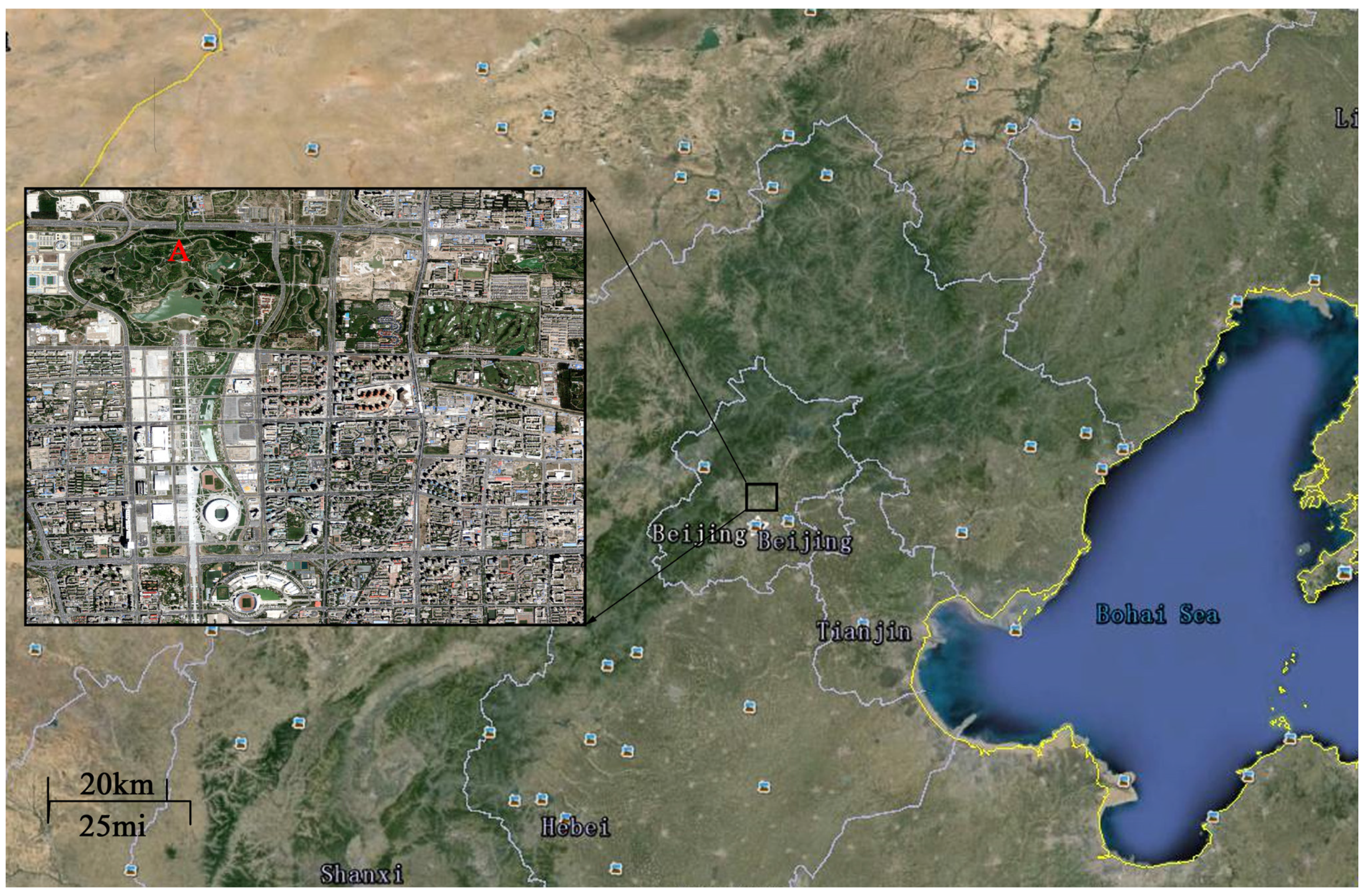
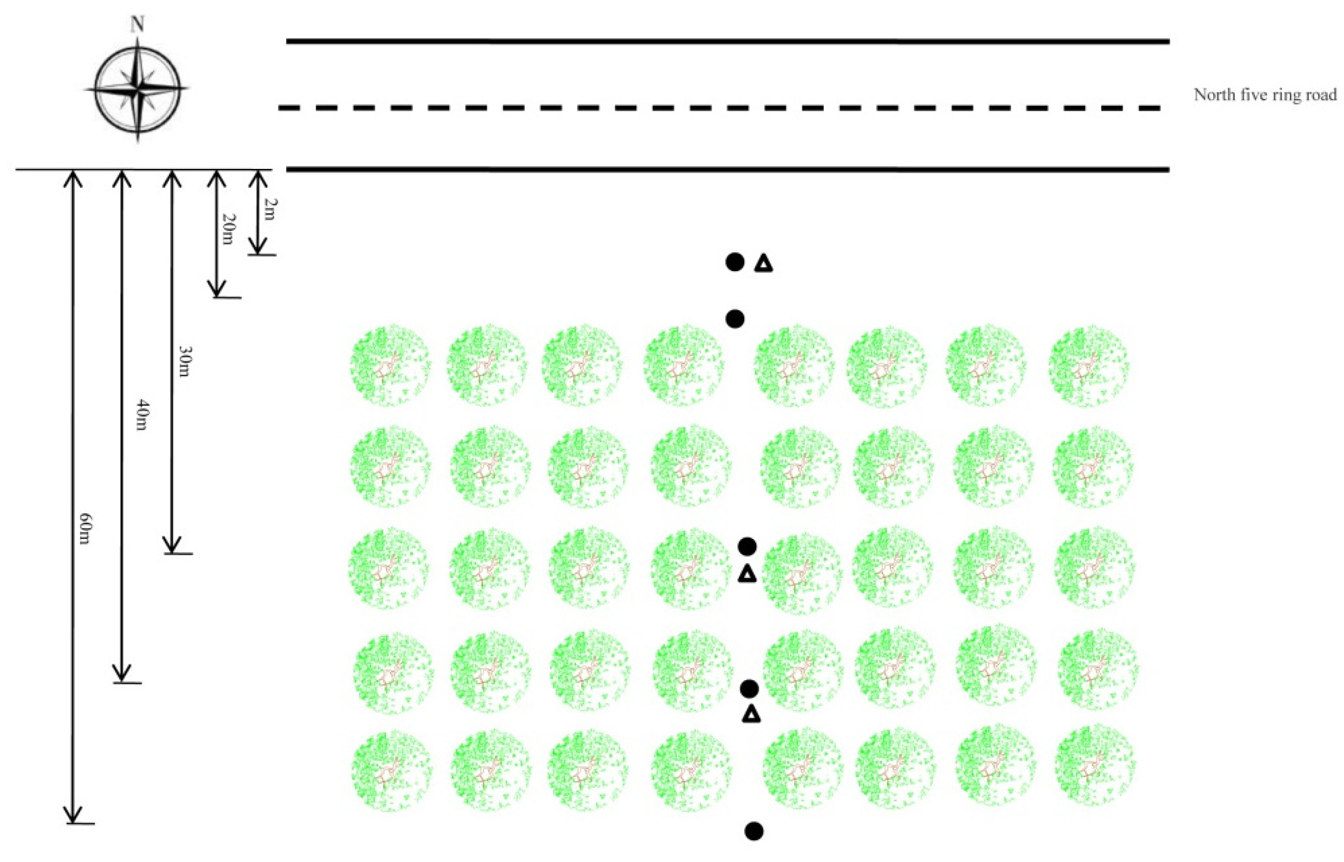
2.1. Study Area


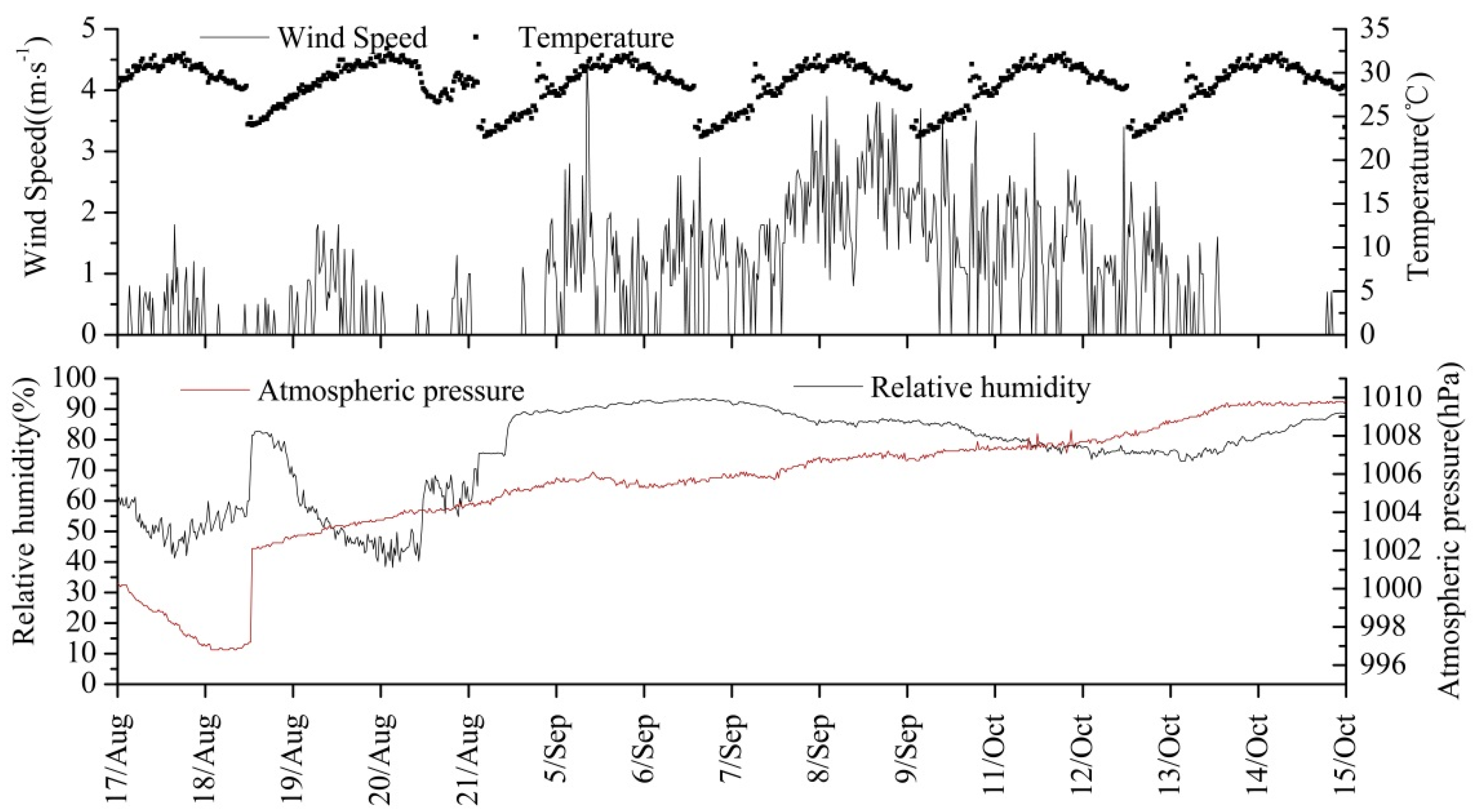
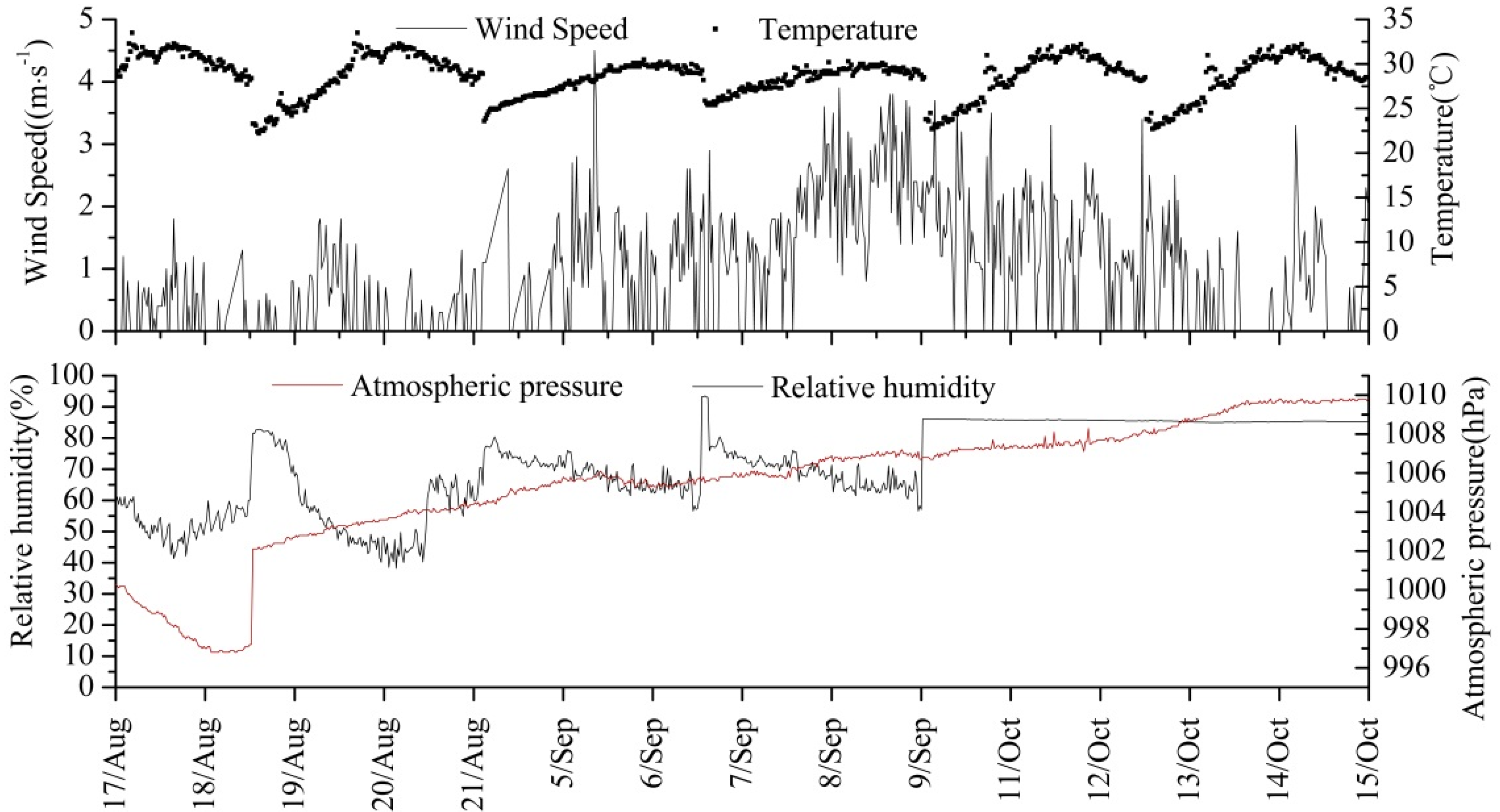
| Time | Inside the Forest Belt | Outside the Forest Belt | ||||
|---|---|---|---|---|---|---|
| Wind Speed (m·s−1) | Temperature (°C) | Relative Humidity (%) | Wind Speed (m·s−1) | Temperature (°C) | Relative Humidity (%) | |
| August 2013 | 0.22 | 28.67 | 58.61 | 0.34 | 29.19 | 57.09 |
| September 2013 | 0.23 | 22.34 | 63.21 | 0.36 | 25.57 | 50.23 |
| October 2013 | 0.32 | 17.22 | 62.43 | 0.42 | 20.13 | 45.57 |
| Time | Inside the Forest Belt | Outside the Forest Belt | ||||
|---|---|---|---|---|---|---|
| Wind Speed (m·s−1) | Temperature (°C) | Relative Humidity (%) | Wind Speed (m·s−1) | Temperature (°C) | Relative Humidity (%) | |
| August 2013 | 0.23 | 29.31 | 56.28 | 0.34 | 29.19 | 57.09 |
| September 2013 | 0.25 | 23.59 | 62.38 | 0.36 | 25.57 | 50.23 |
| October 2013 | 0.342 | 18.45 | 61.80 | 0.42 | 20.13 | 45.57 |

2.2. Collection and Measurement of Particles


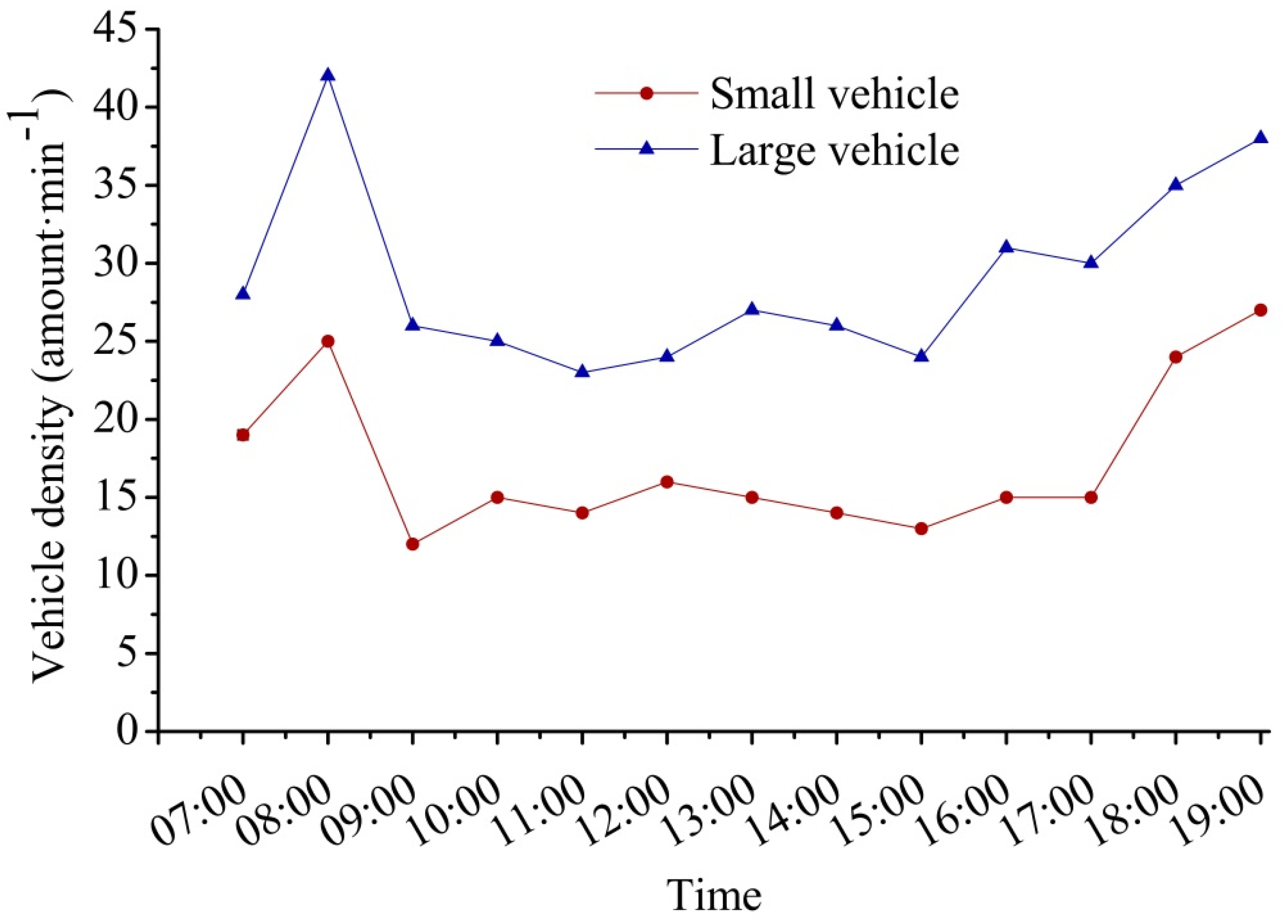
2.3. Urban Forest Effects Model: Air Particulate Removed by Trees
- (1)
- two different tree species of the road shelterbelts; and
- (2)
- shelterbelt area: the areas of the two species are the same with a length of 2000 m and a width of 60 m.
- Vg(populus) = 0.00125(0.5u) (number of observations = 9; p < 0.05: R2 = 0.87)
- Vg(F. chinensis Roxb.) = 0.00178(0.56u) (number of observations = 9; p < 0.05: R2 = 0.80),
3. Results
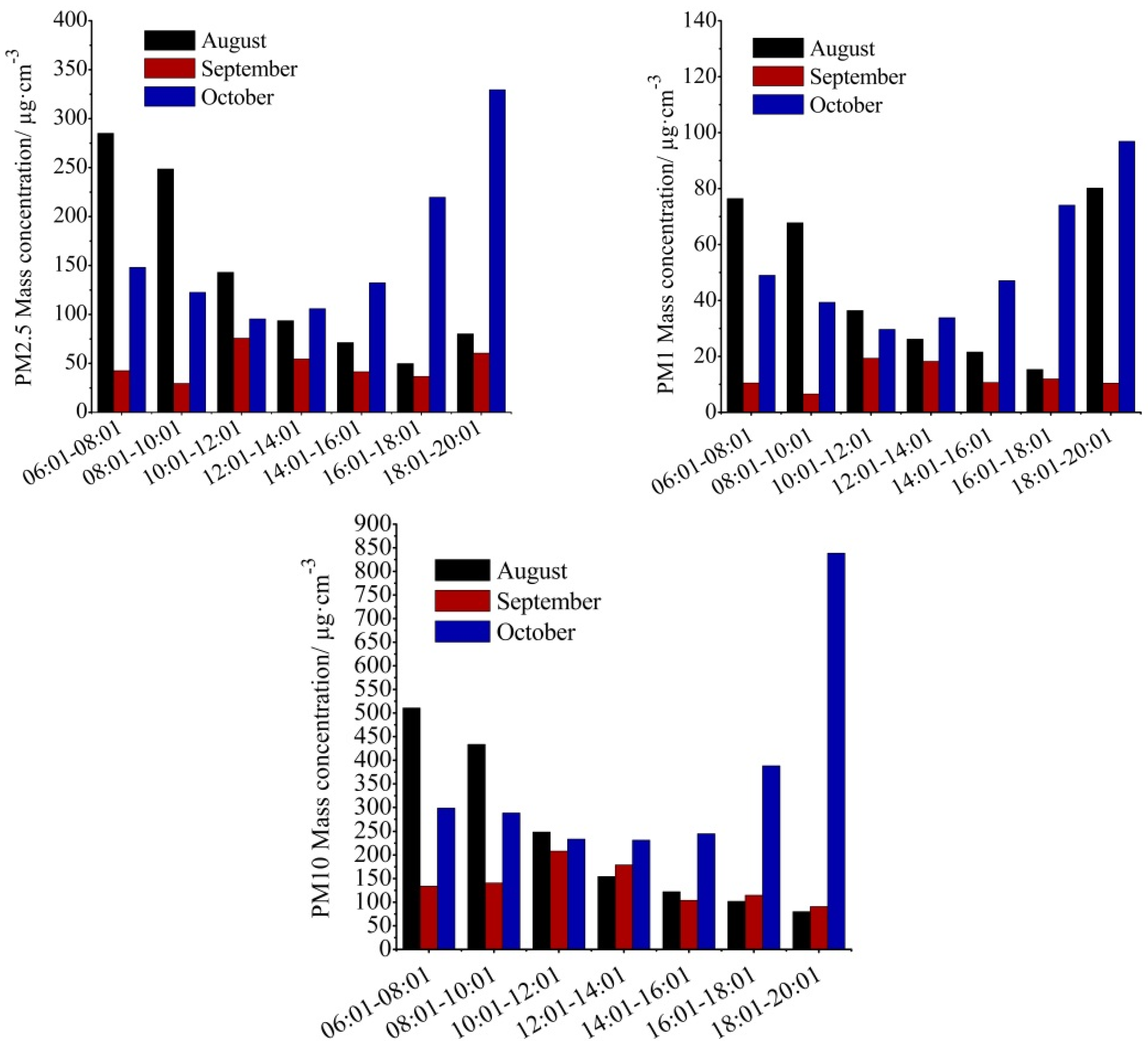
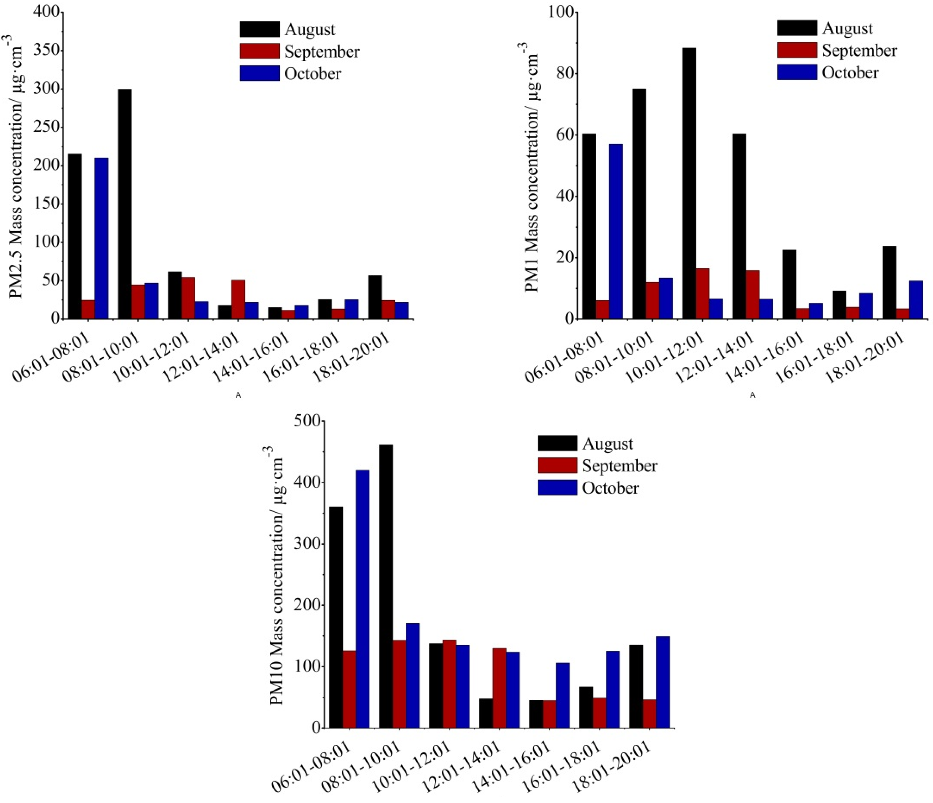
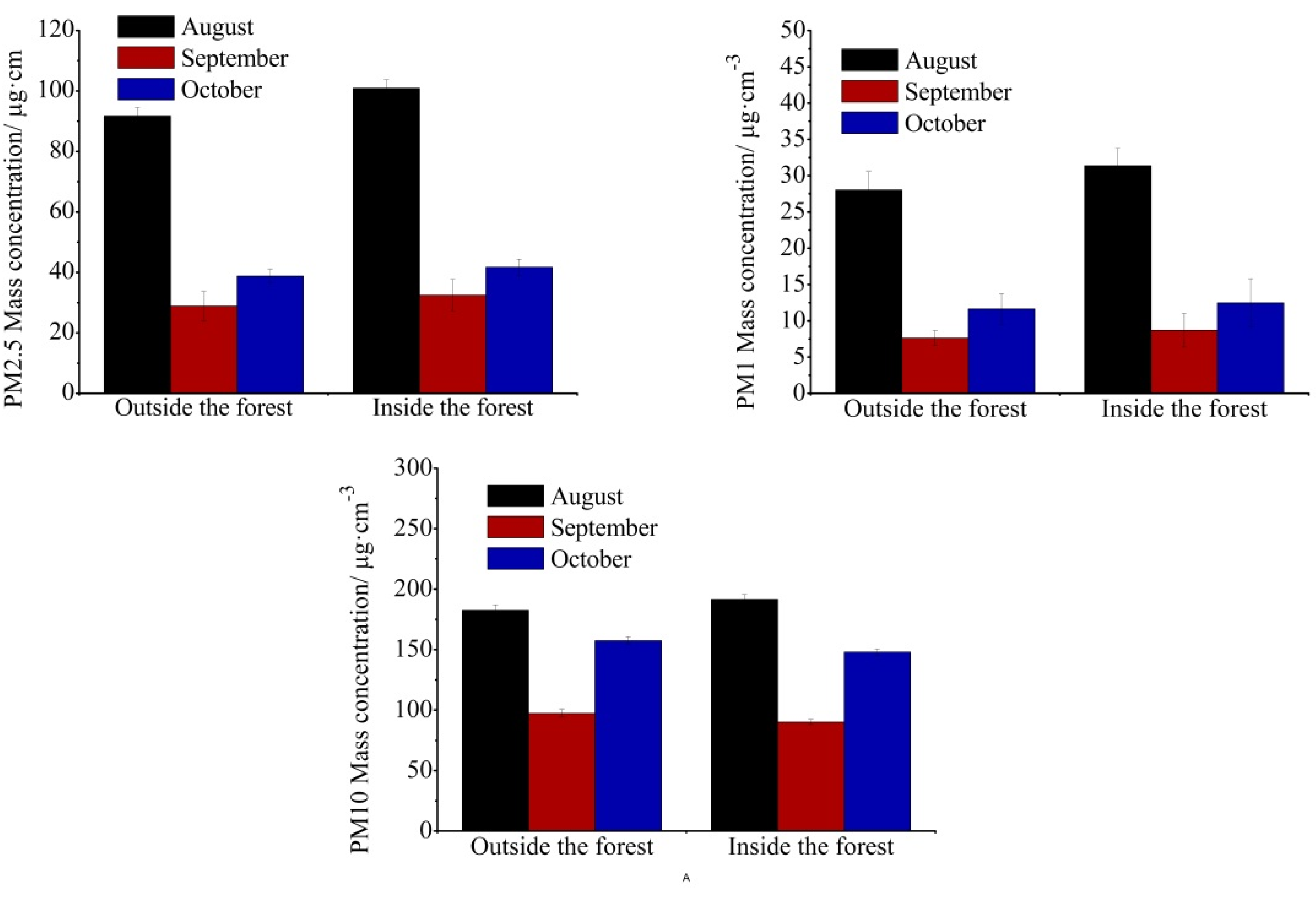
3.1. Temporal Variation in Particulate Mass Concentration inside Shelterbelts


| Shelterbelt/Month | PM2.5/TSP | PM1/TSP | PM10/TSP | PM1/PM10 | PM2.5/PM10 | PM1/PM2.5 | |||||||
|---|---|---|---|---|---|---|---|---|---|---|---|---|---|
| Mean | SD | Mean | SD | Mean | SD | Mean | SD | Mean | SD | Mean | SD | ||
| Populus tomentosa | August | 0.44 | 0.04 | 0.15 | 0.09 | 0.75 | 0.11 | 0.19 | 0.13 | 0.59 | 0.14 | 0.33 | 0.04 |
| September | 0.27 | 0.01 | 0.07 | 0.13 | 0.82 | 0.11 | 0.09 | 0.09 | 0.55 | 0.04 | 0.27 | 0.01 | |
| October | 0.36 | 0.11 | 0.12 | 0.11 | 0.77 | 0.07 | 0.15 | 0.12 | 0.47 | 0.11 | 0.32 | 0.02 | |
| Mean | 0.36 | 0.05 | 0.11 | 0.11 | 0.78 | 0.10 | 0.14 | 0.11 | 0.54 | 0.10 | 0.31 | 0.02 | |
| Fraxinus chinensis Roxb. | August | 0.49 | 0.12 | 0.14 | 0.01 | 0.84 | 0.08 | 0.17 | 0.07 | 0.58 | 0.05 | 0.29 | 0.03 |
| September | 0.19 | 0.05 | 0.05 | 0.04 | 0.57 | 0.05 | 0.08 | 0.02 | 0.55 | 0.04 | 0.25 | 0.01 | |
| October | 0.25 | 0.07 | 0.07 | 0.02 | 0.94 | 0.13 | 0.08 | 0.02 | 0.39 | 0.03 | 0.30 | 0.04 | |
| Mean | 0.31 | 0.08 | 0.09 | 0.02 | 0.78 | 0.09 | 0.11 | 0.04 | 0.51 | 0.04 | 0.28 | 0.03 | |
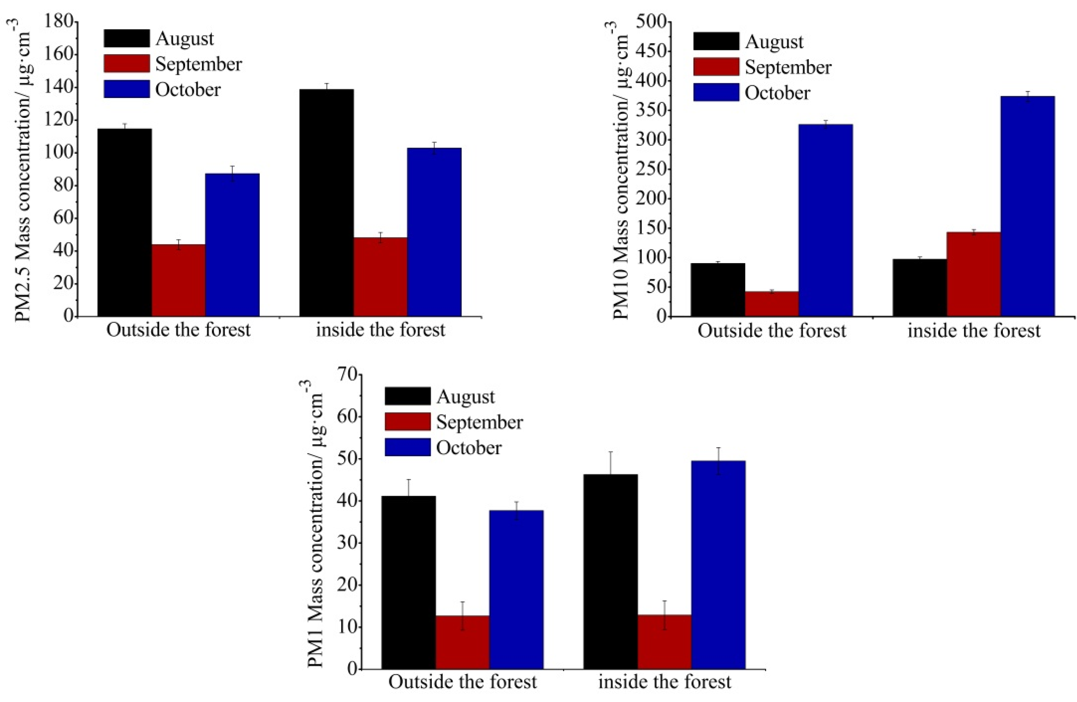
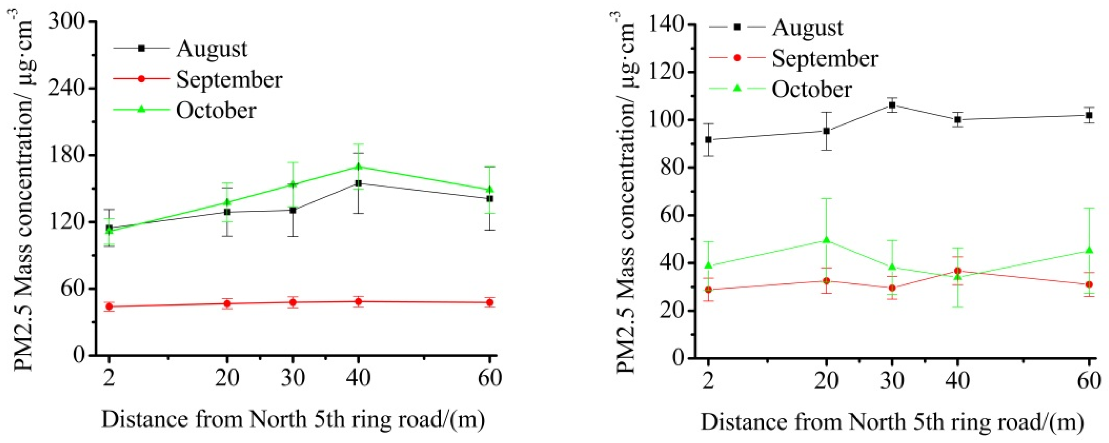
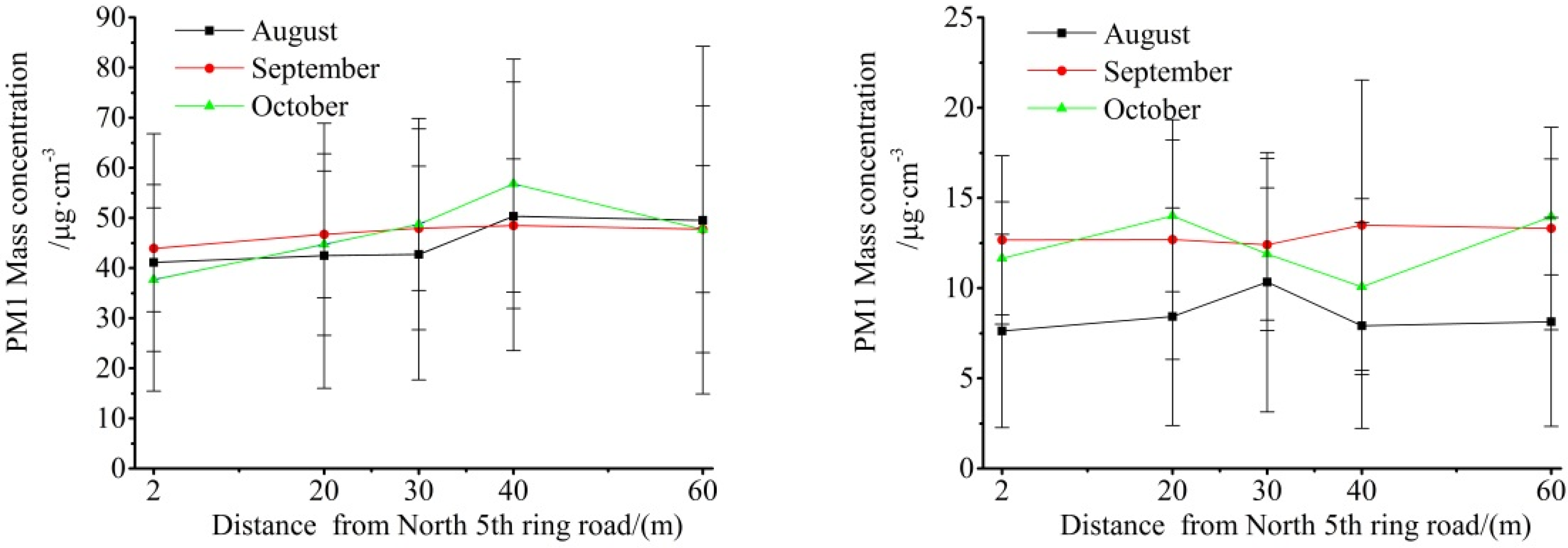
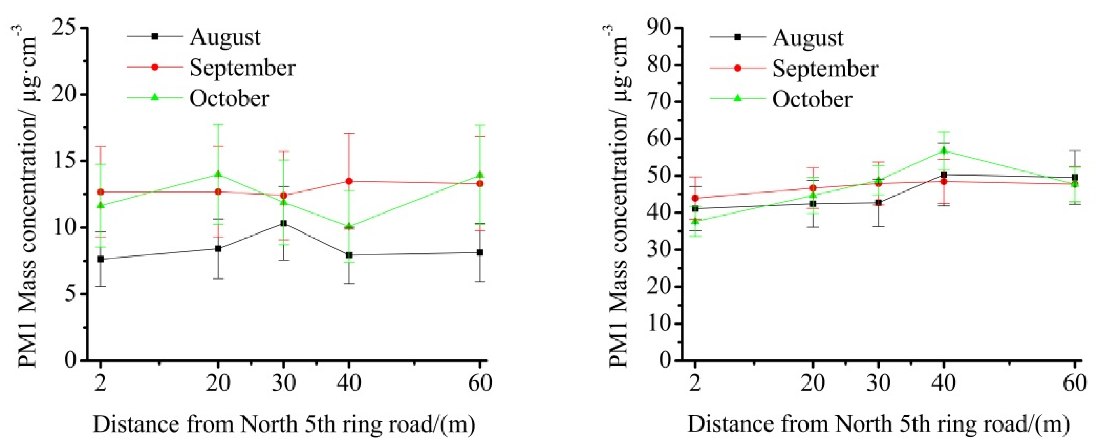
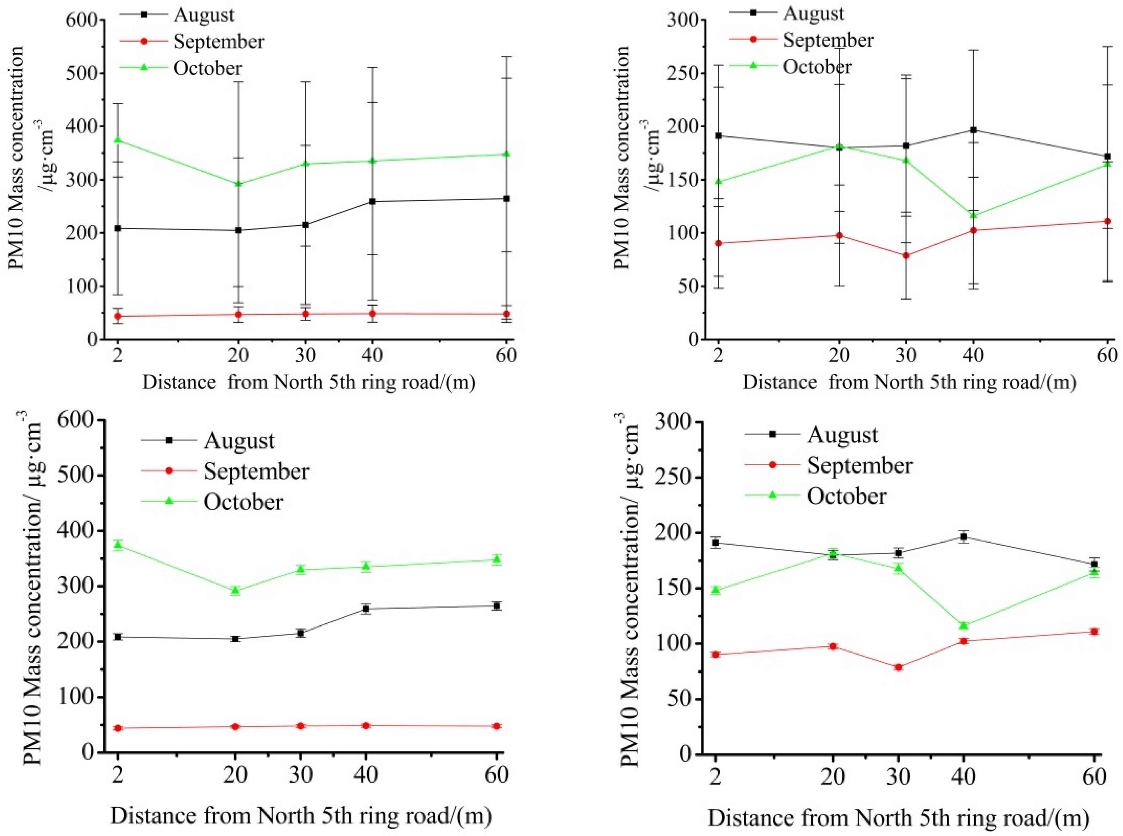
3.2. Particulate Mass Concentration Variation in Different Locations outside and inside Shelterbelts


| Meteorological Elements | Spearman Correlation Coefficients | Two-Tailed Significance Level |
|---|---|---|
| Wind speed | −0.779 * | 0.020 |
| Temperature | −0.755 ** | 0.000 |
| Relative humidity | 0.804 ** | 0.000 |
| Atmospheric pressure | 0.506 ** | 0.000 |
| Meteorological Elements | Spearman Correlation Coefficients | Two-Tailed Significance Level |
|---|---|---|
| Wind speed | −0.226 ** | 0.006 |
| Temperature | −0.798 ** | 0.000 |
| Relative humidity | 0.657 ** | 0.000 |
| Atmospheric pressure | 0.090 | 0.276 |


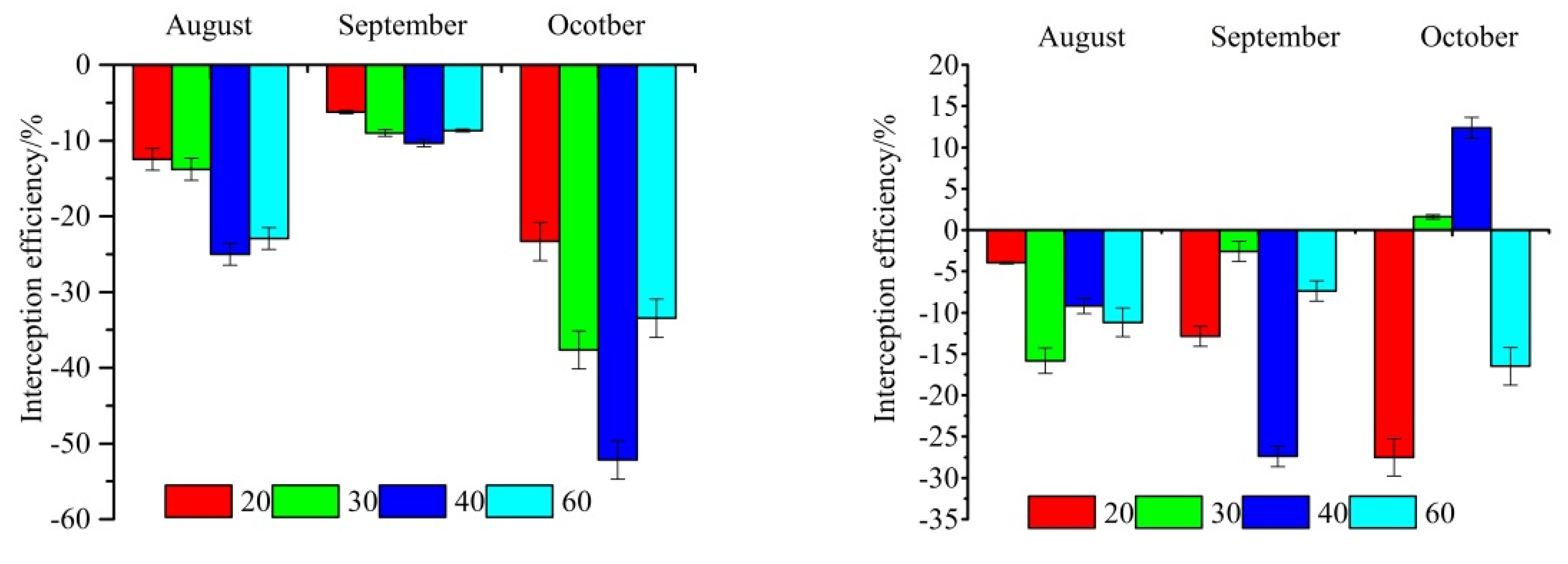
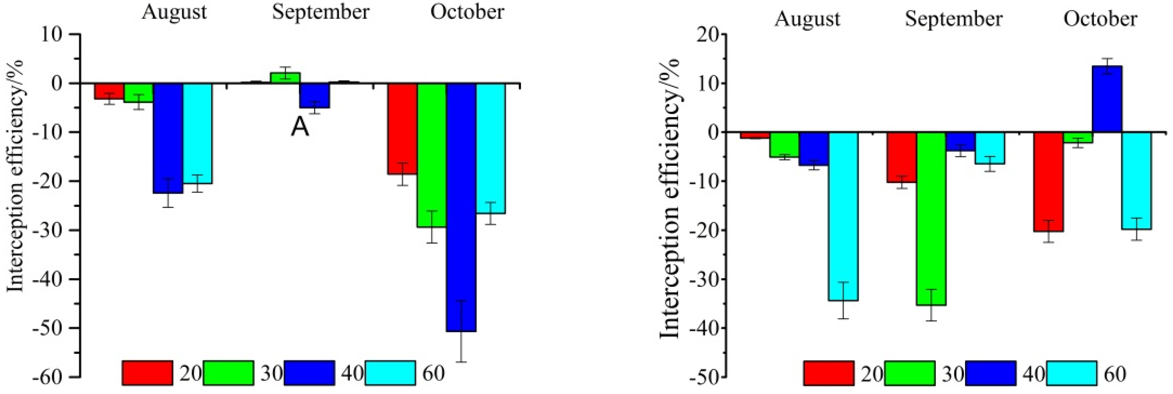
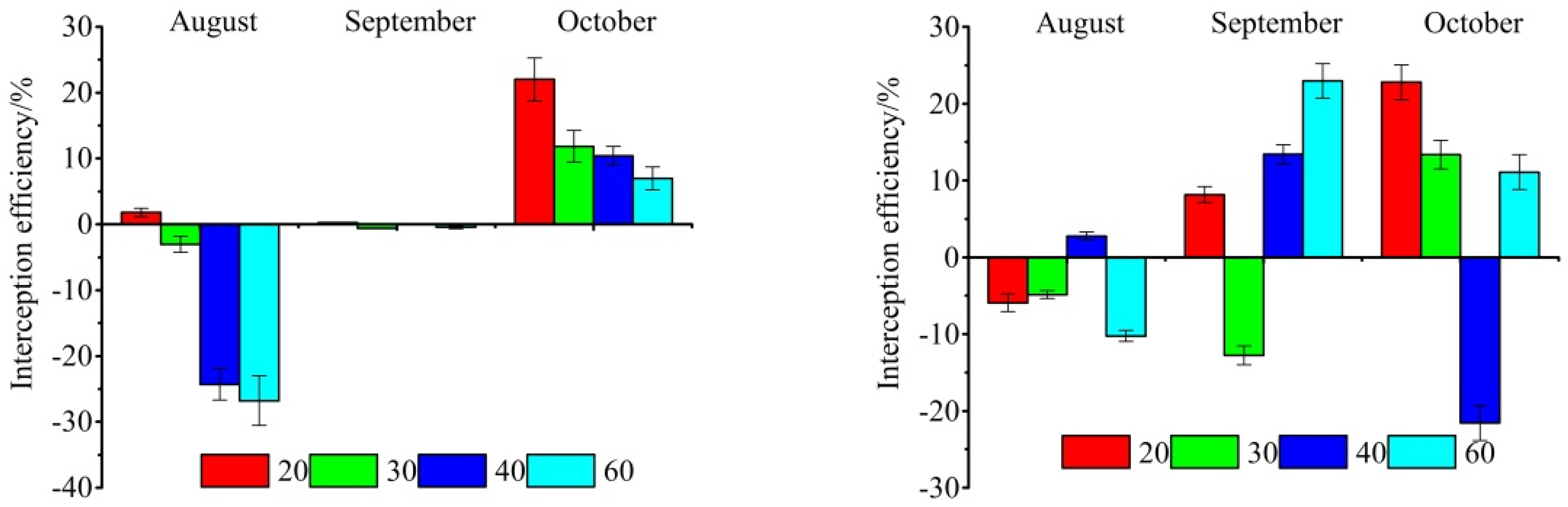
3.3. Particulate Removal Efficiency


3.4. Air-Pollutant Removal


4. Discussion
5. Conclusions
- (1)
- The particle mass concentration inside the shelterbelts presented a single peak or bimodal distribution (peaks at 08:00 and 12:00) and lower mass concentrations at other times.
- (2)
- The particle mass concentration inside the shelterbelt is higher than outside.
- (3)
- The particle interception efficiency of the two forest belts over the three months in descending order was PM10 > PM1 > PM2.5.
- (4)
- The two shelterbelts captured air pollutants at rates of 1496.285 and 909.075 kg/month. Based on monthly average concentrations and pollutant capture quantities, the major atmospheric pollutant in Beijing city is PM10.
Acknowledgments
Author Contributions
Conflicts of Interest
References
- Maher, B.A.; Ahmed, I.A.; Davison, B.; Karloukovski, V.; Clarke, R. Impact of roadside tree lines on indoor concentrations of traffic-derived particulate matter. Environ. Sci. Technol. 2013, 47, 13737–13744. [Google Scholar] [CrossRef] [PubMed]
- Sæbø, A.; Popek, R.; Nawrot, B.; Gawrorńska, H.; Sæbø, A.; Gawroński, S.W. Plant species differnces in particulate matter accumulation on leaf surfaces. Sci. Total Environ. 2012, 427–428, 347–354. [Google Scholar] [CrossRef] [PubMed]
- Nizzetto, L.; Cassani, C.; di Guardo, A. Deposition of PCBs in mountains: The forest filter effect of different forest ecosystem types. Ecotoxicol. Environ. Saf. 2006, 63, 75–83. [Google Scholar] [CrossRef] [PubMed]
- Nowak, D.J. Air pollution removal by Chicago’s urban fores. In Chicago’s Urban Forest Ecosystem: Results of the Chicago Urban Forest Climate Project; McPherson, E.G., Nowak, D.J., Rowntree, R.A., Eds.; U.S. Department of Agriculture, Forest Service, Northeastern Forest Experiment Station: Radnor, PA, USA, 1994; pp. 63–82. [Google Scholar]
- Beckett, K.P.; Freer-Smith, P.H.; Taylor, G. The capture of particulate pollution by trees at five contrasting urban sites. Arbor J. 2000, 24, 209–230. [Google Scholar] [CrossRef]
- Fowler, D.; Skiba, U.; Nemitz, E.; Choubedar, F.; Branford, D.; Donovan, R.; Rowland, P. Measuring aerosol and heavy metal deposition on urban woodland and grassusing inventories of 210 Pb and metal concentrations in soil. Water Air Soil Pollut. 2004, 4, 483–499. [Google Scholar] [CrossRef]
- Freer-Smith, P.H.; Beckett, K.P.; Taylor, G. Deposition velocities to Sorbus aria, Acer campestre, Populus deltoides × trichocarpa ‘Beaupre’, Pinus nigra and × Cupressocyparis leylandii for coarse, fine and ultra-fine particles in the urban environment. Environ. Pollut. 2005, 133, 157–167. [Google Scholar] [CrossRef] [PubMed]
- Tiwary, A.; Sinnett, D.; Peachy, C.; Chalabi, Z.; Vurdoulakis, S.; Fletcher, T.; Leonardi, G.; Grundy, C.; Azapagic, A.; Hutchings, T.R. An integrated tool to assess the role of new planting in PM10 capture and thehuman health benefits: A case study in London. Environ. Pollut. 2009, 157, 2645–2653. [Google Scholar] [CrossRef] [PubMed]
- Nowak, D.J.; Hirabayashi, S.; Bodine, A.; Hoehn, R.E. Modeled PM2.5 removal by trees in ten U.S. cities and associated health Effects. Environ. Pollut. 2013, 178, 395–402. [Google Scholar] [CrossRef] [PubMed]
- McDonald, A.G.; Bealey, W.J.; Fowler, D.; Dragosits, U.; Skiba, U.; Smith, R.I.; Donovan, R.G.; Brett, H.E.; Hewitt, C.N.; Nemitz, E.; et al. Quantifying the effect of urban tree planting on concentrations and depositions of PM10 in two UK conurbations. Atmos. Environ. 2007, 41, 8455–8467. [Google Scholar] [CrossRef]
- Robinson, M.S.; Zhao, M.; Zack, L.; Brindley, C.; Portz, L.; Quarterman, M.; Long, X.; Herckes, P. Characterization of PM2.5 collected during broadcast and slash-pile prescribed burns of predominately ponderosa pine forests in northern Arizona. Atmos. Environ. 2011, 45, 2087–2094. [Google Scholar] [CrossRef]
- Matsuda, K.; Fujimura, Y.; Hayashi, K.; Takahashi, A.; Nakaya, K. Deposition velocity of PM2.5 sulfate in the summer above a deciduous forest in central Japan. Atmos. Environ. 2010, 44, 4582–4587. [Google Scholar] [CrossRef]
- Beckett, K.P.; Freer, P.H.; Taylor, G. Urban woodlands: Their role in reducing the effects of particulate pollution. Environ. Pollut. 1998, 99, 347–360. [Google Scholar] [CrossRef] [PubMed]
- Beckett, K.P.; Freer-Smith, P.H.; Taylor, G. Particulate pollution capture by urban trees: Effect of species and windspeed. Glob. Chang. Biol. 2000, 6, 995–1003. [Google Scholar] [CrossRef]
- Tallis, M.; Taylor, G.; Sinnett, D.; Freer-smith, P. Estimating the removal of atmospheric particulate pollution by the urban tree canopy of London, under current and future environments. Landsc. Urban Plan. 2011, 103, 129–138. [Google Scholar] [CrossRef]
- Gallagher, M.W.; Nemitz, E.; Dorsey, J.R.; Fowler, D.; Sutton, M.A. Measurements and parameterizations of small aerosol deposition velocities to grassland, arable crops, and forest: Influence of surface roughness length on deposition. J. Geophys. Res. 2002, 107, 1–10. [Google Scholar]
- Gregory, P.H. The Microbiology of the Atmosphere; Leonard Hill: New York, NY, USA, 1973. [Google Scholar]
- Decker, E.H.; Elliott, S.; Smith, F.A.; Blake, D.R.; Rowland, F.S. Energy and material flow through the urban ecosystem. Annu. Rev. Energy Environ. 2000, 25, 685–740. [Google Scholar] [CrossRef]
- Urbat, M.; Lehndorff, E.; Schwark, L. Biomonitoring of air quality in the Cologne conurbation using pine needles as a passive sampler—Part I: Magnetic properties. Atmos. Environ. 2004, 38, 3781–3792. [Google Scholar] [CrossRef]
- Fowler, D.; Cape, T.N.; Unsworth, M.H. Deposition of atmospheric pollutants on forests. Philos. Trans. R. Soc. Lond. 1989, 324, 247–265. [Google Scholar] [CrossRef]
- Reinap, A.; Wiman, B.; Svenningsson, B.; Gunnarsson, S. Oak leaves as aerosol collectors: Relationship with wind velocity and particle size distribution. Experiment results and their implications. Trees 2009, 23, 1263–1274. [Google Scholar] [CrossRef]
- Popek, R.; Gawrorńska, H.; Sæbø, A.; Wrochna, M.; Gawroński, S.W. Particulate matter on foliage of 13 woody species: Deposition on surfaces and phytostabilisation in waxes—A 3-year study. Int. J. Phytoremediation 2013, 15, 245–256. [Google Scholar] [CrossRef] [PubMed]
- Sternberg, T.; Viles, H.; Cathersides, A.; Edwards, M. Dust particulate absorption by ivy (Hedera helix L) on historic walls in urban environments. Sci. Total Environ. 2010, 409, 162–168. [Google Scholar] [CrossRef] [PubMed]
- Hinds, W.C. Aerosol Technology: Properties, Behavior, and Measurement of Airborne Particles, 2nd ed.; Wiley: New York, NY, USA, 1999. [Google Scholar]
- Yin, S.; Shen, Z.; Zhou, P.; Zou, X.; Che, S.; Wang, W. Quantifying air pollution attenuation within urban parks: An experimental approach in Shanghai, China. Environ. Pollut. 2011, 159, 2155–2163. [Google Scholar] [CrossRef] [PubMed]
- Terzaghi, E.; Wild, E.; Zacchello, G.; Cerabolini, B.E.L.; Jones, K.; Guardo, A.D. Forest Filter Effect: Role of leaves in capturing/releasing air particulate matter and its associated PAHs. Atmos. Environ. 2013, 74, 378–384. [Google Scholar] [CrossRef]
- Song, Y.S.; Maher, B.A.; Li, F.; Wang, X.K.; Sun, X.; Zhang, H.X. Particulate matter deposited on leaf of five evergreen species in Beijing, China: Source identification and size distribution. Atmos. Environ. 2015, 105, 53–60. [Google Scholar] [CrossRef]
- Rai, P.K. Environmental magnetic studies of particulates with special reference to biomagnetic monitoring using roadside plant leaves. Atmos. Environ. 2013, 72, 113–129. [Google Scholar] [CrossRef]
- Treshow, M.; Bell, J.N.B. Air Pollution and Plant Life; Wiley: New York, NY, USA, 2002; p. 34. [Google Scholar]
- Lin, M.; Khlystov, A. Investigation of ultrafine particle deposition to vegetation branches in a wind tunnel. Aerosol Sci. Technol. 2012, 46, 465–472. [Google Scholar] [CrossRef]
- Räsänen, J.V.; Holopainen, T.; Joutsensaari, J.; Ndam, C.; Pasanen, P.; Rinnan, Å.; Kivimäenpää, M. Effects of species-specific leaf characteristics and reduced water availability on fine particle capture efficiency of trees. Environ. Pollut. 2013, 183, 64–70. [Google Scholar]
- Räsänen, J.V.; Yli-Pirilä, P.; Holopainen, T.; Joutsensaari, J.; Pasanen, P.; Kivimäenpää, M. Soil drought increases atmospheric fine particle capture efficiency of Norway spruce. Boreal Environ. Res. 2012, 17, 21–30. [Google Scholar]
- Joureva, V.A.; Johnson, D.L.; Hassett, J.P.; Nowak, D.J. Differences in accumulation of PAHs and metals on the leaves of Tilia × euchlora and Pyrus calleryana. Environ. Pollut. 2002, 120, 331–338. [Google Scholar] [CrossRef] [PubMed]
- Dzierzanowski, K.; Popek, R.; Gawronska, H.; Saebø, A.; Gawronski, S.W. Deposition of particulate matter of different size fractions on leaf surfaces and in waxes of urban forest species. Int. J. Phytoremediation 2011, 13, 1037–1046. [Google Scholar] [CrossRef] [PubMed]
- Buccolieri, R.; Gromke, C.; Sabatino, S.D.; Ruck, B. Aerodynamic effects of trees on pollutant concentration in street canyons. Sci. Total Environ. 2009, 407, 5247–5256. [Google Scholar] [CrossRef] [PubMed]
- Sander, H.; Polasky, S.; Haight, R.G. The value of urban tree cover: A hedonic property price model in Ramsey and Dakota Counties, Minnesota, USA. Ecol. Econ. 2010, 69, 1646–1656. [Google Scholar] [CrossRef]
- Litschke, T.; Kuttler, W. On the reduction of urban particle concentration by vegetation—A review. Meteorol. Z. 2008, 17, 229–240. [Google Scholar] [CrossRef]
- Bealey, W.J.; McDonald, A.G.; Nemitz, R.; Donovan, R.; Dragosits, U.; Duffy, T.R.; Fowler, D. Estimating the reduction of urban PM10 concentrations by trees within an environmental information system for planners. J. Environ. Manag. 2007, 85, 44–58. [Google Scholar] [CrossRef]
- Zhang, H.; Ying, Q. Secondary organic aerosol formation and source apportionment in Southeast Texas. Atmos. Environ. 2011, 45, 3217–3227. [Google Scholar] [CrossRef]
- Liao, H.; Zhang, Y.; Chen, W.T.; Raes, F.; Seinfeld, J.H. Effect of chemistryaerosol-climate coupling on predictions of future climate and future levels of tropospheric ozone and aerosols. J. Geophys. Res. Atmos. 2009, 114, D10306. [Google Scholar] [CrossRef]
- Poschl, U. Atmospheric aerosols: Composition, transformation, climate and health effects. Angew. Chem. Int. Ed. 2005, 44, 7520–7540. [Google Scholar] [CrossRef]
- Raupach, M.R.; Woods, N.; Dorr, G.; Leys, J.F.; Cleugh, H.A. The entrapment of particles by windbreaks. Atmos. Environ. 2001, 35, 3373–3383. [Google Scholar] [CrossRef]
- Wilson, J.D. Deposition of particles to a thin windbreak: The effect of a gap. Atmos. Environ. 2005, 39, 5525–5531. [Google Scholar] [CrossRef]
- Bouvet, T.; Loubet, B.; Wilson, J.; Tuzet, A. Filtering of windborne particles by a natural windbreak. Bound.-Layer Meteorol. 2007, 123, 481–509. [Google Scholar] [CrossRef]
- Killus, J.P.; Meyer, J.P.; Durran, D.R.; Anderson, G.E.; Jerskey, T.N.; Reynolds, S.D.; Ames, J. Continued Research in Mesoscale Air Pollution Simulation Modeling. Volume V: Refinements in Numerical Analysis, Transport, Chemistry, and Pollutant Removal; EPN60013-841095a; Environmental Protection Agency: Research Triangle Park, NC, USA, 1984; p. 221. [Google Scholar]
- Nieuwstadt, F. The Turbulent Structure of the Stable, Noctural Boundary Layer. J. Atmos. Sci. 1984, 41, 2202–2216. [Google Scholar]
- Panofsky, H.A.; Dutton, J.A. Atmospheric Turbulence; Wiley: New York, NY, USA, 1984. [Google Scholar]
- Zannetti, P. Air Pollution Modeling; Van Nostrand Reinhold: New York, NY, USA, 1990. [Google Scholar]
- Pasquill, F. The estimation of the dispersion of windbourne material. Meteorol. Mag. 1961, 90, 33–49. [Google Scholar]
- Van Ulden, A.P.; Holtslag, A.A.M. Estimation of atmospheric boundary layer parameters for diffusion application. J. Clim. Appl. Meteorol. 1985, 24, 1196–1207. [Google Scholar]
- Dyer, A.J.; Braley, C.F. An alternative analysis of flux gradient relationships. Boundary-layer Meteorol. 1982, 22, 3–19. [Google Scholar] [CrossRef]
- Pederson, J.R.; Massman, W.J.; Mahrt, L.; Delany, A.; Oncley, S.; den Hartog, G.; Neumann, H.H.; Mickle, R.E.; Shaw, R.H.; Paw, U.K.T.; et al. California ozone deposition experiment: Methods, results, and opportunities. Atmos. Environ. 1995, 29, 3115–3132. [Google Scholar] [CrossRef]
- Freer-Smith, P.H.; El-Khatib, A.A.; Taylor, G. Capture of particulate pollution by trees: A comparison of species typical of semi-arid areas (Ficus nitida and Eucalyptus globulus) with European and North American species. Water Air Soil Pollut. 2004, 155, 173–187. [Google Scholar] [CrossRef]
- Slinn, W.G.N. Predictions for particle deposition to vegetation canopies. Atmos. Environ. 1982, 16, 1785–1794. [Google Scholar] [CrossRef]
- Kwiecien, M. Deposition of inorganic particulate aerosols to vegetation—A new method of estimating. Environ. Monit. Assess. 1997, 46, 191–207. [Google Scholar] [CrossRef]
- Pullman, M. Conifer PM2.5 Deposition and Re-Suspension in Wind and Rain Events. Master’s Thesis, Cornell University, Ithaca, NY, USA, 2009; p. 51. [Google Scholar]
- Sun, F.; Yin, Z.; Lun, X.; Zhao, Y.; Li, R.; Shi, F.; Yu, X. Deposition Velocity of PM2.5 in the Winter and Spring above Deciduous and Coniferous Forests in Beijing, China. PLoS ONE 2014, 9, 1–11. [Google Scholar] [CrossRef]
- White, E.J.; Turner, J. A method for estimating income of nutrients in a catch of airborne particles by a woodland canopy. J. Appl. Ecol. 1970, 7, 441–461. [Google Scholar] [CrossRef]
- Yang, J.; McBride, J.; Zhou, J.; Sun, Z. The urban forest in Beijing and its role in air pollution reduction. Urban For. Urban Green. 2005, 3, 65–78. [Google Scholar] [CrossRef]
- Nguyen, T.; Yu, X.; Zhang, Z.; Liu, M.; Liu, X. Relationship between types of urban forest and PM2.5 capture at three growth stages of leaves. J. Environ. Sci. 2015, 27, 33–41. [Google Scholar] [CrossRef]
- Wu, Z.P.; Wang, C.; Xu, J.N.; Hu, L.X. Air-borne anions and particulate matter in six urban green spaces during the summer. J. Tsinghua Univ. Sci. Technol. 2007, 47, 2152–2157. [Google Scholar]
- Islam, M.N.; Rahman, K.S.; Bahar, M.M.; Habib, M.A.; Ando, K.; Hattori, N. Pollution attenuation by roadside greenbelt in and around urban areas. Urban For. Urban Green. 2012, 11, 460–464. [Google Scholar] [CrossRef]
- Li, C.-S.; Lin, C.-H. PM1/PM2.5/PM10 characteristics in the urban atmosphere of Taipei. Aerosol Sci. Technol. 2002, 36, 469–473. [Google Scholar] [CrossRef]
- Gomišček, B.; Hauck, H.; Stopper, S.; Preining, O. Spatial and temporal variations of PM1, PM2.5, PM10 andparticle number concentration during the AUPHEP—Project. Atmos. Environ. 2004, 38, 3917–3934. [Google Scholar] [CrossRef]
- Yang, F.M.; He, K.B.; Ma, Y.L.; Zhang, Q.; Yu, X.C. Variation characteristics of PM2.5 concentration and its relationship with PM10 and TSP in Beijing. China Environ. Sci. 2002, 22, 506–511. [Google Scholar]
- Zhu, T.Z.; Guan, D.X.; Zhou, G.S.; Jin, C.J. Review of ecological effect research of farmland sheltbelts. In Theory of Eco-engineering of Farmland Protective Plantation; Chinese Forestry Press: Beijing, China, 2001; pp. 91–92. [Google Scholar]
- Telenta, M.; Duhovnik, J.; Kosel, F.; Šajn, V. Numerical and experimental study of the flow through a geometrically accurate porous wind barrier model. J. Wind Eng. Ind. Aerodyn. 2014, 124, 99–108. [Google Scholar] [CrossRef]
- Plate, E.J. The aerodynamics of shelterbelts. Agric. Meteorol. 1971, 8, 203–211. [Google Scholar]
- Huang, L.M.; Chan, H.C.; Lee, J.-T. A numerical study on flow around nonuniform porous fences. J. Appl. Math. 2012, 12, 1–12. [Google Scholar]
- Mori, J.; Hanslin, H.M.; Burchi, G.; Sæbø, A. Particulate matter and element accumulation on coniferous trees at different distances from a highway. Urban For. Urban Greening 2015, 14, 170–177. [Google Scholar] [CrossRef]
- Lovett, G.M. Atmospheric deposition of nutrients and pollutants in North America: An ecological perspective. Ecol. Appl. 1994, 4, 629–650. [Google Scholar] [CrossRef]
- Powe, N.A.; Willis, K.G. Mortality and morbidity benefits of air pollution (SO2 and PM10) absorption attributable to woodland in Britain. J. Environ. Manag. 2004, 70, 119–128. [Google Scholar] [CrossRef]
- McPherson, E.G.; Nowak, D.J.; Rowntree, R.E. Chicago’s Urban Forest Ecosystem: Results of the Chicago Urban Forest Climate Project; USDA General Training Report NE-186; Northeastern Forest Experiment Station: Radnor, PA, USA, 1994. [Google Scholar]
- Nowak, D.J.; Crane, D.E.; Stevens, J.C. Air pollution removal by urban trees and shrubs in the United States. Urban For. Urban Greening 2006, 4, 115–123. [Google Scholar] [CrossRef]
- Graustein, W.C.; Turekian, K.K. The effects of forests and topography on the deposition of sub-micrometer aerosols measured by lead-210 and cesium-137 in soils. Agric. For. Meteorol. 1989, 47, 199–220. [Google Scholar] [CrossRef]
- Ould-Dada, Z.; Baghini, N.M. Resuspension of small particles from tree surfaces. Atmos. Environ. 2001, 35, 3799–3809. [Google Scholar] [CrossRef]
- Tiwary, A.; Reff, A.; Colls, J.J. Collection of ambient particulate matter by porous vegetation barriers: Sampling and characterization methods. J. Aerosol Sci. 2008, 39, 40–47. [Google Scholar] [CrossRef]
- Fowler, D. Pollutant deposition and uptake by vegetation. In Air Pollution and Plant Life; Bell, J.N.B., Treshow, M., Eds.; John Wiley and Sons, Ltd.: New York, NY, USA, 2002; pp. 43–67. [Google Scholar]
- Abelsohn, A.; Stieb, D.; Sanborn, M.D.; Weir, E. Indentifying and managing adverse environmental health effects 2: Outdoor air pollution. Can. Med. Assoc. J. 2002, 166, 1161–1167. [Google Scholar]
© 2015 by the authors; licensee MDPI, Basel, Switzerland. This article is an open access article distributed under the terms and conditions of the Creative Commons Attribution license (http://creativecommons.org/licenses/by/4.0/).
Share and Cite
Chen, J.; Yu, X.; Sun, F.; Lun, X.; Fu, Y.; Jia, G.; Zhang, Z.; Liu, X.; Mo, L.; Bi, H. The Concentrations and Reduction of Airborne Particulate Matter (PM10, PM2.5, PM1) at Shelterbelt Site in Beijing. Atmosphere 2015, 6, 650-676. https://doi.org/10.3390/atmos6050650
Chen J, Yu X, Sun F, Lun X, Fu Y, Jia G, Zhang Z, Liu X, Mo L, Bi H. The Concentrations and Reduction of Airborne Particulate Matter (PM10, PM2.5, PM1) at Shelterbelt Site in Beijing. Atmosphere. 2015; 6(5):650-676. https://doi.org/10.3390/atmos6050650
Chicago/Turabian StyleChen, Jungang, Xinxiao Yu, Fenbing Sun, Xiaoxiu Lun, Yanlin Fu, Guodong Jia, Zhengming Zhang, Xuhui Liu, Li Mo, and Huaxing Bi. 2015. "The Concentrations and Reduction of Airborne Particulate Matter (PM10, PM2.5, PM1) at Shelterbelt Site in Beijing" Atmosphere 6, no. 5: 650-676. https://doi.org/10.3390/atmos6050650