
A Review on Predicting Ground PM2.5 Concentration Using Satellite Aerosol Optical Depth


Abstract
:1. Introduction
2. Methods
2.1. Subject of This Review
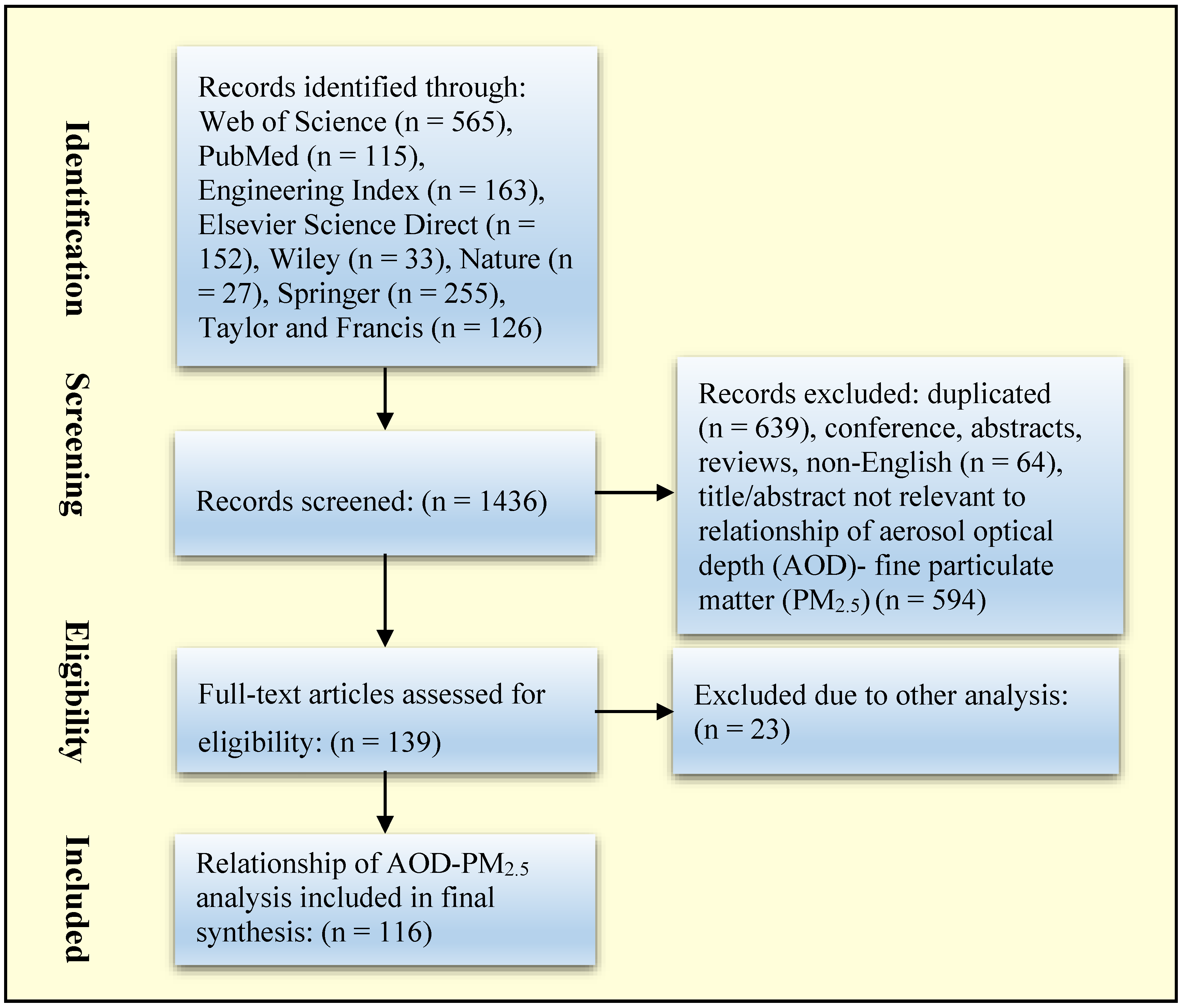
2.2. Search Criteria
2.3. Inclusion and Exclusion Criteria
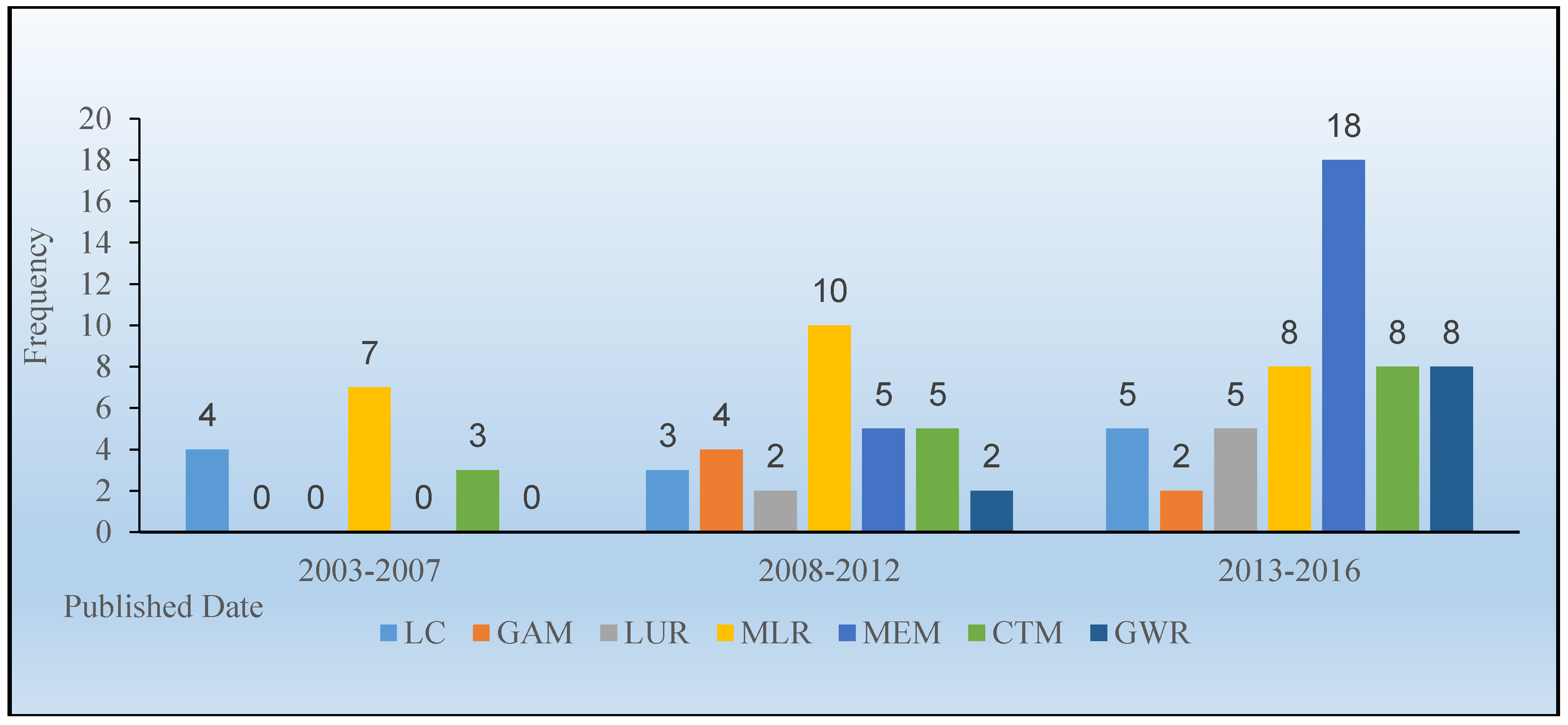
3. Results
4. Discussion
4.1. Multiple Linear Regression
4.1.1. Theory Background and Application
4.1.2. Advantages and Disadvantages
4.2. Mixed-Effect Model
4.2.1. Theory Background and Application
4.2.2. Advantages and Disadvantages
4.3. Chemistry Transport Model
4.3.1. Theory Background and Application
4.3.2. Advantages and Disadvantages
4.4. Geographical Weighted Regression
4.4.1. Theory Background and Application
4.4.2. Advantages and Disadvantages
4.5 Other Models
4.6. Summary
5. Conclusions
Acknowledgments
Author Contributions
Conflicts of Interest
Abbreviations
| AOD | Aerosol Optical Depth |
| MODIS | Moderate Resolution Imaging Spectrometer |
| MISR | Multi-Angle Imaging Spectrometer |
| GEOS | Geostationary Operational Environment Satellite |
| SeaWiFS | Sea-viewing Wide Field-of-view Sensor |
| POLDER | Polarization of Earth’s Reflectance and Directionality |
| CALIOP | Cloud-Aerosol Lidar with Orthogonal Polarization |
| GOCI | Geostationary Ocean Color Imager |
| OMI | Ozone Monitoring Instrument (OMI) |
| AATSR | Advanced Along-Track Scanning Radiometer |
| MERIS | Medium Resolution Imaging Spectrometer |
| LC | Linear Correlations |
| MLR | Multiple Linear Regression |
| LUR | Land Use Regression |
| GAM | Generalized Additive Model |
| MEM | Mixed-Effect Model |
| CTM | Chemical Transport Model |
| GLM | General Linear regression Model |
| GWR | Geographically weighted regression |
| TWR | Temporally Weighted Regression |
| GTWR | Geographically and Temporally Weighted Regression |
| ANN | Artificial Neural Networks |
| SVR | Support Vector Regression |
| MCA | Maximum Covariance Analysis |
| CMCA | Combined Maximum Covariance Analysis |
| TVM | Two-variate method |
| MVM | Multivariate method |
| OLS | Ordinary Least Squares model |
| TSM | Two-Stage Model |
| MAIAC | Multi-Angle Implementation of Atmospheric Correction algorithm |
| DSA | Deletion/Substitution/Addition |
| BMEM | Bayesian Maximum Entropy method |
| Nested MEM | Nested Mixed-Effect Model |
| Non-nested MEM | Non-nested Mixed-Effect Model |
| SEC | Surface Extinction Coefficient |
| BTH | Beijing-Tianjin-Hebei region |
| PRD | Pearl River Delta region |
| YRD | Yangtze River Delta region |
| NARR | North American Regional Reanalysis |
| NLDAS | North American Land Data Assimilation System |
| Sample-based CV-R2 | Sample-based Cross Validated-coefficient of determination |
| DOY-based CV-R2 | Day-of-Year-based Cross Validated-coefficient of determination |
References
- World Health Organization. 7 Milion Premature Death in Annually Linked to Air Pollution. Available online: http://www.who.int/mediacentre/news/releases/2014/air-pollution/en/ (accessed on 25 March 2014).
- Dockery, D.W. Heath effects of particulate air pollution. Ann. Epidemiol. 2009, 19, 257–263. [Google Scholar] [CrossRef] [PubMed]
- Risom, L.; Moller, P.; Loft, S. Oxidative stress-induced DNA damage by particulate air pollution. Mutat. Res. 2005, 592, 119–137. [Google Scholar] [CrossRef] [PubMed]
- Hoek, G.; Krishnan, R.M.; Beelen, R.; Peters, A.; Ostro, B.; Brunekreef, B.; Kaufman, J.D. Long-term air pollution exposure and cardio-respiratory mortality: A review. Environ. Health 2013, 12, 43. [Google Scholar] [CrossRef] [PubMed]
- Brook, R.D.; Rajagopalan, S.; Pope, C.A., 3rd; Brook, J.R.; Bhatnagar, A.; Diez-Roux, A.V.; Holguin, F.; Hong, Y.; Luepker, R.V.; Mittleman, M.A.; et al. Particulate matter air pollution and cardiovascular disease: An update to the scientific statement from the american heart association. Circulation 2010, 121, 2331–2378. [Google Scholar] [CrossRef] [PubMed]
- Lim, S.S.; Vos, T.; Flaxman, A.D.; Danaei, G.; Shibuya, K.; Adair-Rohani, H.; Amann, M.; Anderson, H.R.; Andrews, K.G.; Aryee, M.; et al. A comparative risk assessment of burden of disease and injury attributable to 67 risk factors and risk factor clusters in 21 regions, 1990–2010: A systematic analysis for the global burden of disease study 2010. Lancet 2012, 380, 2224–2260. [Google Scholar] [CrossRef]
- Lee, M.; Kloog, I.; Chudnovsky, A.; Lyapustin, A.; Wang, Y.; Melly, S.; Coull, B.; Koutrakis, P.; Schwartz, J. Spatiotemporal prediction of fine particulate matter using high-resolution satellite images in the southeastern U.S. 2003–2011. J. Expo. Sci. Environ. Epidemiol. 2016, 26, 377–384. [Google Scholar] [CrossRef] [PubMed]
- Sinha, P.R.; Gupta, P.; Kaskaoutis, D.G.; Sahu, L.K.; Nagendra, N.; Manchanda, R.K.; Kumar, Y.B.; Sreenivasan, S. Estimation of particulate matter from satellite- and ground-based observations over Hyderabad, India. Int. J. Remote Sens. 2015, 36, 6192–6213. [Google Scholar] [CrossRef]
- Mordukhovich, I.; Coull, B.; Kloog, I.; Koutrakis, P.; Vokonas, P.; Schwartz, J. Exposure to sub-chronic and long-term particulate air pollution and heart rate variability in an elderly cohort: The normative aging study. Environ. Health 2015, 14, 1–10. [Google Scholar] [CrossRef] [PubMed]
- Liu, D.-J.; Li, L. Application study of comprehensive forecasting model based on entropy weighting method on trend of PM2.5 concentration in Guangzhou, China. Int. J. Environ. Res. Public Health 2015, 12, 7085–7099. [Google Scholar] [CrossRef] [PubMed]
- Gupta, P.; Christopher, S.A. An evaluation of Terra-MODIS sampling for monthly and annual particulate matter air quality assessment over the southeastern United States. Atmos. Environ. 2008, 42, 6465–6471. [Google Scholar] [CrossRef]
- Lee, M.; Koutrakis, P.; Coull, B.; Kloog, I.; Schwartz, J. Acute effect of fine particulate matter on mortality in three southeastern states from 2007–2011. J. Expo. Sci. Environ. Epidemiol. 2015. [Google Scholar] [CrossRef] [PubMed]
- Liu, Y.; Koutrakis, P.; Kahn, R. Estimating fine particulate matter component concentrations and size distributions using satellite-retrieved fractional aerosol optical depth: Part 2—A case study. J. Air Waste Manag. Assoc. 2007, 57, 1360–1369. [Google Scholar] [PubMed]
- Zhang, Y.L.; Cao, F. Fine particulate matter (PM2.5) in china at a city level. Sci. Rep. 2015, 5, 14884. [Google Scholar] [CrossRef] [PubMed]
- Liu, Y. New directions: Satellite driven PM2.5 exposure models to support targeted particle pollution health effects research. Atmos. Environ. 2013, 42, 6465–6471. [Google Scholar] [CrossRef]
- Wang, J. Intercomparison between satellite-derived aerosol optical thickness and PM2.5 mass: Implications for air quality studies. Geophys. Res. Lett. 2003, 30. [Google Scholar] [CrossRef]
- Tao, J.; Zhang, M.; Chen, L.; Wang, Z.; Su, L.; Ge, C.; Han, X.; Zou, M. A method to estimate concentrations of surface-level particulate matter using satellite-based aerosol optical thickness. Sci. China Earth Sci. 2013, 56, 1422–1433. [Google Scholar] [CrossRef]
- Liu, Y. Mapping annual mean ground-level PM2.5 concentrations using multiangle imaging spectroradiometer aerosol optical thickness over the contiguous United States. J. Geophys. Res. 2004, 109. [Google Scholar] [CrossRef]
- Lee, H.J.; Liu, Y.; Coull, B.A.; Schwartz, J.; Koutrakis, P. A novel calibration approach of MODIS AOD data to predict PM2.5 concentrations. Atmos. Chem. Phys. Discuss. 2011, 11, 9769–9795. [Google Scholar] [CrossRef]
- Liu, Y.; Franklin, M.; Kahn, R.; Koutrakis, P. Using aerosol optical thickness to predict ground-level PM2.5 concentrations in the St. Louis area: A comparison between MISR and MODIS. Remote Sens. Environ. 2007, 107, 33–44. [Google Scholar] [CrossRef]
- Zhang, H.; Hoff, R.M.; Engel-Cox, J.A. The relation between moderate resolution imaging spectroradiometer (MODIS) aerosol optical depth and PM2.5 over the United States: A geographical comparison by U.S. Environmental Protection Agency regions. J. Air Waste Manag. Assoc. 2009, 59, 1358–1369. [Google Scholar] [CrossRef] [PubMed]
- Liu, Y.; Koutrakis, P.; Kahn, R. Estimating fine particulate matter component concentrations and size distributions using satellite-retrieved fractional aerosol optical depth: Part 1—Method development. J. Air Waste Manag. Assoc. 2007, 57, 1351–1359. [Google Scholar] [PubMed]
- Liu, Y.; Paciorek, C.J.; Koutrakis, P. Estimating regional spatial and temporal variability of PM2.5 concentrations using satellite data, meteorology, and land use information. Environ. Health Perspect. 2009, 117, 886–892. [Google Scholar] [CrossRef] [PubMed]
- Paciorek, C.J.; Liu, Y.; Moreno-Macias, H.; Kondragunta, S. Spatiotemporal associations between goes aerosol optical depth retrievals and ground-level PM2.5. Environ. Sci. Technol. 2008, 42, 5800–5806. [Google Scholar] [CrossRef] [PubMed]
- Leon, J.-F.; Liousse, C.; Galy-Lacaux, C.; Doumbia, T.; Cachier, H. Monitoring of ambient fine particulate matter concentrations from space: application to European and African cities. Proc. SPIE 2010, 78262A. [Google Scholar] [CrossRef]
- Kacenelenbogen, M.; Leon, J.F.; Chiapello, I.; Tanre, D. Characterization of aerosol pollution events in France using ground-based and polder–2 satellite data. Atmos. Chem. Phys. 2006, 6, 4843–4849. [Google Scholar] [CrossRef]
- Van Donkelaar, A.; Martin, R.V.; Brauer, M.; Boys, B.L. Use of satellite observations for long-term exposure assessment of global concentrations of fine particulate matter. Environ. Health Perspect. 2015, 123, 135–143. [Google Scholar] [CrossRef] [PubMed]
- Lary, D.J.; Faruque, F.S.; Malakar, N.; Moore, A.; Roscoe, B.; Adams, Z.L.; Eggelston, Y. Estimating the global abundance of ground level presence of particulate matter (PM2.5). Geosp. Health 2014, 7, S611–S630. [Google Scholar] [CrossRef] [PubMed]
- Li, J.; Carlson, B.E.; Lacis, A.A. How well do satellite AOD observations represent the spatial and temporal variability of PM2.5 concentration for the United States? Atmos. Environ. 2015, 102, 260–273. [Google Scholar] [CrossRef]
- Toth, T.D.; Zhang, J.; Campbell, J.R.; Hyer, E.J.; Reid, J.S.; Westphal, D.L. Impact of data quality and surface-to-column representativeness on the PM2.5/satellite AOD relationship for the contiguous United States. Atmos. Chem. Phys. Discuss. 2014, 14, 6049–6062. [Google Scholar] [CrossRef] [Green Version]
- Engel-Cox, J.A.; Holloman, C.H.; Coutant, B.W.; Hoff, R.M. Qualitative and quantitative evaluation of MODIS satellite sensor data for regional and urban scale air quality. Atmos. Environ. 2004, 38, 2495–2509. [Google Scholar] [CrossRef]
- Hu, Z. Spatial analysis of MODIS aerosol optical depth, PM2.5, and chronic coronary heart disease. Int. J. Health Geogr. 2009, 8, 27. [Google Scholar] [CrossRef] [PubMed]
- Kloog, I.; Koutrakis, P.; Coull, B.A.; Lee, H.J.; Schwartz, J. Assessing temporally and spatially resolved PM2.5 exposures for epidemiological studies using satellite aerosol optical depth measurements. Atmos. Environ. 2011, 45, 6267–6275. [Google Scholar] [CrossRef]
- Kloog, I.; Nordio, F.; Coull, B.A.; Schwartz, J. Incorporating local land use regression and satellite aerosol optical depth in a hybrid model of spatiotemporal PM2.5 exposures in the mid-atlantic states. Environ. Sci. Technol. 2012, 46, 11913–11921. [Google Scholar] [CrossRef] [PubMed]
- Chudnovsky, A.A.; Lee, H.J.; Kostinski, A.; Kotlov, T.; Koutrakis, P. Prediction of daily fine particulate matter concentrations using aerosol optical depth retrievals from the Geostationary Operational Environmental Satellite (GOES). J. Air Waste Manag. Assoc. 2012, 62, 1022–1031. [Google Scholar] [CrossRef] [PubMed]
- Higgs, G.; Sterling, D.A.; Aryal, S.; Vemulapalli, A.; Priftis, K.N.; Sifakis, N.I. Aerosol optical depth as a measure of particulate exposure using imputed censored data, and relationship with childhood asthma hospital admissions for 2004 in Athens, Greece. Environ. Health Insights 2015, 9, 27–33. [Google Scholar] [CrossRef] [PubMed]
- Hutchison, K.D.; Smith, S.; Faruqui, S.J. Correlating MODIS aerosol optical thickness data with ground-based PM2.5 observations across Texas for use in a real-time air quality prediction system. Atmos. Environ. 2005, 39, 7190–7203. [Google Scholar] [CrossRef]
- Liu, Y.; Sarnat, J.A.; Kilaru, V.; Jacob, D.J.; Koutrakis, P. Estimating ground-level PM2.5 in the eastern United States using satellite remote sensing. Environ. Sci. Technol. 2005, 39, 3269–3278. [Google Scholar] [CrossRef] [PubMed]
- Chu, D.A. Analysis of the relationship between MODIS aerosol optical depth and PM2.5 in the summertime US. Proc. SPIE 2006, 6299, 629903. [Google Scholar]
- Engel-Cox, J.A.; Hoff, R.M.; Rogers, R.; Dimmick, F.; Rush, A.C.; Szykman, J.J.; Al-Saadi, J.; Chu, D.A.; Zell, E.R. Integrating lidar and satellite optical depth with ambient monitoring for 3-dimensional particulate characterization. Atmos. Environ. 2006, 40, 8056–8067. [Google Scholar] [CrossRef]
- Gupta, P.; Christopher, S.A.; Wang, J.; Gehrig, R.; Lee, Y.; Kumar, N. Satellite remote sensing of particulate matter and air quality assessment over global cities. Atmos. Environ. 2006, 40, 5880–5892. [Google Scholar] [CrossRef]
- Koelemeijer, R.B.A.; Homan, C.D.; Matthijsen, J. Comparison of spatial and temporal variations of aerosol optical thickness and particulate matter over Europe. Atmos. Environ. 2006, 40, 5304–5315. [Google Scholar] [CrossRef]
- Van Donkelaar, A.; Martin, R.V.; Park, R.J. Estimating ground-level PM2.5 using aerosol optical depth determined from satellite remote sensing. J. Geophys. Res. 2006, 111. [Google Scholar] [CrossRef]
- Kumar, N.; Chu, A.; Foster, A. An empirical relationship between PM2.5 and aerosol optical depth in Delhi metropolitan. Atmos. Environ. 2007, 41, 4492–4503. [Google Scholar] [CrossRef] [PubMed]
- Wallace, J.; Kanaroglou, P. An investigation of air pollution in southern Ontario, Canada, with MODIS and MISR aerosol data. Int. Geosci. Remote Sens. 2007, 4311–4314. [Google Scholar]
- Gupta, P.; Christopher, S.A. Seven year particulate matter air quality assessment from surface and satellite measurements. Atmos. Chem. Phys. 2008, 8, 3311–3324. [Google Scholar] [CrossRef]
- Hutchison, K.D.; Faruqui, S.J.; Smith, S. Improving correlations between MODIS aerosol optical thickness and ground-based PM2.5 observations through 3D spatial analyses. Atmos. Environ. 2008, 42, 530–543. [Google Scholar] [CrossRef]
- Kumar, N.; Chu, A.; Foster, A. Remote sensing of ambient particles in Delhi and its environs: Estimation and validation. Int. J. Remote Sens. 2008, 29, 3383–3405. [Google Scholar] [CrossRef] [PubMed]
- Al-Hamdan, M.Z.; Crosson, W.L.; Limaye, A.S.; Rickman, D.L.; Quattrochi, D.A.; Estes, M.G.; Qualters, J.R.; Sinclair, A.H.; Tolsma, D.D.; Adeniyi, K.A.; et al. Methods for characterizing fine particulate matter using ground observations and remotely sensed data: Potential use for environmental public health surveillance. J. Air Waste Manag. Assoc. 2009, 59, 865–881. [Google Scholar] [CrossRef] [PubMed]
- Green, M.; Kondragunta, S.; Ciren, P.; Xu, C. Comparison of GEOS and MODIS aerosol optical depth (AOD) to aerosol robotic network (AERONET) AOD and improve PM2.5 mass at Bondville, Illinois. J. Air Waste Manag. Assoc. 2009, 59, 1082–1091. [Google Scholar] [CrossRef] [PubMed]
- Gupta, P.; Christopher, S.A. Particulate matter air quality assessment using integrated surface, satellite, and meteorological products: Multiple regression approach. J. Geophys. Res. 2009, 114. [Google Scholar] [CrossRef]
- Gupta, P.; Christopher, S.A. Particulate matter air quality assessment using integrated surface, satellite, and meteorological products: 2. A neural network approach. J. Geophys. Res. 2009, 114. [Google Scholar] [CrossRef]
- Paciorek, C.J.; Liu, Y. Limitations of remotely sensed aerosol as a spatial proxy for fine particulate matter. Environ. Health Perspect. 2009, 117, 904–909. [Google Scholar] [CrossRef] [PubMed]
- Schaap, M.; Apituley, A.; Timmermans, R.M.A.; Koelemeijer, R.B.A.; de Leeuw, G. Exploring the relation between aerosol optical depth and PM2.5 at Cabauw, The Netherlands. Atmos. Chem. Phys. 2009, 9, 909–925. [Google Scholar] [CrossRef]
- Di Nicolantonio, W.; Cacciari, A. Modis multiannual observations in support of air quality monitoring in northern Italy. Ital. J. Remote Sens. Riv. Ital. Telerilevamento 2010, 43, 97–109. [Google Scholar]
- Tian, J.; Chen, D. A semi-empirical model for predicting hourly ground-level fine particulate matter (PM2.5) concentration in southern Ontario from satellite remote sensing and ground-based meteorological measurements. Remote Sens. Environ. 2010, 114, 221–229. [Google Scholar] [CrossRef]
- Van Donkelaar, A.; Martin, R.V.; Brauer, M.; Kahn, R.; Levy, R.; Verduzco, C.; Villeneuve, P.J. Global estimates of ambient fine particulate matter concentrations from satellite-based aerosol optical depth: Development and application. Environ. Health Perspect. 2010, 118, 847–855. [Google Scholar] [CrossRef] [PubMed]
- Wang, Z.; Chen, L.; Tao, J.; Zhang, Y.; Su, L. Satellite-based estimation of regional particulate matter (PM) in Beijing using vertical-and-RH correcting method. Remote Sens. Environ. 2010, 114, 50–63. [Google Scholar] [CrossRef]
- Hu, Z.; Liebens, J.; Rao, K.R. Merging satellite measurement with ground-based air quality monitoring data to assess health effects of fine particulate matter pollution. In Geospatial Analysis of Environmental Health; Maantay, J.A., McLafferty, S., Eds.; Springer: Dordrecht, The Netherlands, 2011; Volume 4, pp. 395–409. [Google Scholar]
- Hystad, P.; Setton, E.; Cervantes, A.; Poplawski, K.; Deschenes, S.; Brauer, M.; van Donkelaar, A.; Lamsal, L.; Martin, R.; Jerrett, M.; et al. Creating national air pollution models for population exposure assessment in Canada. Environ. Health Perspect. 2011, 119, 1123–1129. [Google Scholar] [CrossRef] [PubMed]
- Wu, Y.; Guo, J.; Zhang, X.; Li, X. Correlation between PM concentrations and aerosol optical depth in eastern China based on BP neural networks. In Proceedings of the 2011 IEEE International Geoscience and Remote Sensing Symposium (IGRASS), Vancouver, BC, Canada, 24–29 July 2011.
- Hystad, P.; Demers, P.A.; Johnson, K.C.; Brook, J.; van Donkelaar, A.; Lamsal, L.; Martin, R.; Brauer, M. Spatiotemporal air pollution exposure assessment for a Canadian population-based lung cancer case-control study. Environ. Health 2012, 11, 22. [Google Scholar] [CrossRef] [PubMed]
- Lee, S.J.; Serre, M.L.; van Donkelaar, A.; Martin, R.V.; Burnett, R.T.; Jerrett, M. Comparison of geostatistical interpolation and remote sensing techniques for estimating long-term exposure to ambient PM2.5 concentrations across the continental united states. Environ. Health Perspect. 2012, 120, 1727–1732. [Google Scholar] [CrossRef] [PubMed]
- Lee, H.J.; Coull, B.A.; Bell, M.L.; Koutrakis, P. Use of satellite-based aerosol optical depth and spatial clustering to predict ambient PM2.5 concentrations. Environ. Res. 2012, 118, 8–15. [Google Scholar] [CrossRef] [PubMed]
- Liu, Y.; He, K.; Li, S.; Wang, Z.; Christiani, D.C.; Koutrakis, P. A statistical model to evaluate the effectiveness of PM2.5 emissions control during the Beijing 2008 Olympic Games. Environ. Int. 2012, 44, 100–105. [Google Scholar] [CrossRef] [PubMed]
- Mao, L.; Qiu, Y.; Kusano, C.; Xu, X. Predicting regional space-time variation of PM2.5 with land-use regression model and MODIS data. Environ. Sci. Pollut. Res. Int. 2012, 19, 128–138. [Google Scholar] [CrossRef] [PubMed]
- Van Donkelaar, A.; Martin, R.V.; Pasch, A.N.; Szykman, J.J.; Zhang, L.; Wang, Y.X.; Chen, D. Improving the accuracy of daily satellite-derived ground-level fine aerosol concentration estimates for north America. Environ. Sci. Technol. 2012, 46, 11971–11978. [Google Scholar] [CrossRef] [PubMed]
- Wu, Y.; Guo, J.; Zhang, X.; Tian, X.; Zhang, J.; Wang, Y.; Duan, J.; Li, X. Synergy of satellite and ground based observations in estimation of particulate matter in eastern China. Sci. Total Environ. 2012, 433, 20–30. [Google Scholar] [CrossRef] [PubMed]
- Beckerman, B.S.; Jerrett, M.; Martin, R.V.; van Donkelaar, A.; Ross, Z.; Burnett, R.T. Application of the deletion/substitution/addition algorithm to selecting land use regression models for interpolating air pollution measurements in California. Atmos. Environ. 2013, 77, 172–177. [Google Scholar] [CrossRef]
- Beckerman, B.S.; Jerrett, M.; Serre, M.; Martin, R.V.; Lee, S.J.; van Donkelaar, A.; Ross, Z.; Su, J.; Burnett, R.T. A hybrid approach to estimating national scale spatiotemporal variability of PM2.5 in the contiguous United States. Environ. Sci. Technol. 2013, 47, 7233–7241. [Google Scholar] [PubMed]
- Chudnovsky, A.A.; Kostinski, A.; Lyapustin, A.; Koutrakis, P. Spatial scales of pollution from variable resolution satellite imaging. Environ. Pollut. 2013, 172, 131–138. [Google Scholar] [CrossRef] [PubMed]
- Chudnovsky, A.; Lyapustin, A.; Wang, Y.; Schwartz, J.; Koutrakis, P. Analyses of high resolution aerosol data from MODIS satellite: A MAIAC retrieval, southern New England, US. Proc. SPIE 2013, 8795, 8795E-1. [Google Scholar]
- Cordero, L.; Wu, Y.; Gross, B.M.; Moshary, F. Assessing satellite AOD based and ARF/CMAQ output PM2.5 estimators. Proc. SPIE 2013, 8723, 872319. [Google Scholar]
- Hu, X.; Waller, L.A.; Al-Hamdan, M.Z.; Crosson, W.L.; Estes, M.G., Jr.; Estes, S.M.; Quattrochi, D.A.; Sarnat, J.A.; Liu, Y. Estimating ground-level PM2.5 concentrations in the southeastern U.S. using geographically weighted regression. Environ. Res. 2013, 121, 1–10. [Google Scholar] [CrossRef] [PubMed]
- Kumar, N.; Liang, D.; Comellas, A.; Chu, A.D.; Abrams, T. Satellite-based pm concentrations and their application to copd in Cleveland, OH. J. Expo. Sci. Environ. Epidemiol. 2013, 23, 637–646. [Google Scholar] [CrossRef] [PubMed]
- Saunders, R.O.; Kahl, J.D.W.; Ghorai, J.K. Improved estimation of PM2.5 using lagrangian satellite-measured aerosol optical depth. Atmos. Environ. 2014, 91, 146–153. [Google Scholar] [CrossRef]
- Strawa, A.W.; Chatfield, R.B.; Legg, M.; Scarnato, B.; Esswein, R. Improving retrievals of regional fine particulate matter concentrations from moderate resolution imaging spectroradiometer (MODIS) and ozone monitoring instrument (OMI) multisatellite observations. J. Air Waste Manag. Assoc. 2013, 63, 1434–1446. [Google Scholar] [CrossRef] [PubMed]
- Chang, H.H.; Hu, X.; Liu, Y. Calibrating MODIS aerosol optical depth for predicting daily PM2.5 concentrations via statistical downscaling. J. Expo. Sci. Environ. Epidemiol. 2014, 24, 98–404. [Google Scholar] [CrossRef] [PubMed]
- Chiu, Y.H.M.; Coull, B.A.; Sternthal, M.J.; Kloog, I.; Schwartz, J.; Cohen, S.; Wright, R.J. Effects of prenatal community violence and ambient air pollution on childhood wheeze in an urban population. J. Allergy Clin. Immunol. 2014, 133, 713–722 e714. [Google Scholar] [CrossRef] [PubMed]
- Hu, X.; Waller, L.A.; Lyapustin, A.; Wang, Y.; Al-Hamdan, M.Z.; Crosson, W.L.; Estes, M.G.; Estes, S.M.; Quattrochi, D.A.; Puttaswamy, S.J.; et al. Estimating ground-level PM2.5 concentrations in the southeastern United States using maiac AOD retrievals and a two-stage model. Remote Sens. Environ. 2014, 140, 220–232. [Google Scholar] [CrossRef]
- Hu, X.; Waller, L.A.; Lyapustin, A.; Wang, Y.; Liu, Y. 10-year spatial and temporal trends of PM2.5 concentrations in the southeastern us estimated using high-resolution satellite data. Atmos. Chem. Phys. Discuss. 2014, 14, 6301–6314. [Google Scholar] [CrossRef]
- Kloog, I.; Chudnovsky, A.A.; Just, A.C.; Nordio, F.; Koutrakis, P.; Coull, B.A.; Lyapustin, A.; Wang, Y.; Schwartz, J. A new hybrid spatio-temporal model for estimating daily multi-year PM2.5 concentrations across northeastern USA using high resolution aerosol optical depth data. Atmos. Environ. 2014, 95, 581–590. [Google Scholar] [CrossRef]
- Kloog, I.; Nordio, F.; Zanobetti, A.; Coull, B.A.; Koutrakis, P.; Schwartz, J.D. Short term effects of particle exposure on hospital admissions in the Mid-Atlantic States: A population estimate. PLoS ONE 2014, 9, e88578. [Google Scholar] [CrossRef] [PubMed]
- Kim, H.-S.; Chung, Y.-S.; Kim, J.-T. Spatio-temporal variations of optical properties of aerosols in East Asia measured by MODIS and relation to the ground-based mass concentrations observed in central Korea during 2001 similar to 2010. Asia Pac. J. Atmos. Sci. 2014, 50, 191–200. [Google Scholar] [CrossRef]
- Lai, H.K.; Tsang, H.; Thach, T.Q.; Wong, C.M. Health impact assessment of exposure to fine particulate matter based on satellite and meteorological information. Environ. Sci. Process Impacts 2014, 16, 239–246. [Google Scholar] [CrossRef] [PubMed]
- Lee, H.J.; Kang, C.M.; Coull, B.A.; Bell, M.L.; Koutrakis, P. Assessment of primary and secondary ambient particle trends using satellite aerosol optical depth and ground speciation data in the New England region, United States. Environ. Res. 2014, 133, 103–110. [Google Scholar] [CrossRef] [PubMed]
- Ma, Z.; Hu, X.; Huang, L.; Bi, J.; Liu, Y. Estimating ground-level PM2.5 in China using satellite remote sensing. Environ. Sci. Technol. 2014, 48, 7436–7444. [Google Scholar] [CrossRef] [PubMed]
- Rush, A.C.; Dougherty, J.J.; Engel-Cox, J.A. Correlating seasonal averaged in-situ monitoring of fine PM with satellite remote sensing data using geographic information system (GIS). Proc. SPIE 2014, 5547, 91–102. [Google Scholar]
- Song, W.; Jia, H.; Huang, J.; Zhang, Y. A satellite-based geographically weighted regression model for regional PM2.5 estimation over the Pearl River Delta region in China. Remote Sens. Environ. 2014, 154, 1–7. [Google Scholar] [CrossRef]
- Chan, S.H.; van Hee, V.C.; Bergen, S.; Szpiro, A.A.; DeRoo, L.A.; London, S.J.; Marshall, J.D.; Kaufman, J.D.; Sandler, D.P. Long-term air pollution exposure and blood pressure in the sister study. Environ. Health Perspect. 2015, 123, 951–958. [Google Scholar] [CrossRef] [PubMed]
- Coker, E.; Ghosh, J.; Jerrett, M.; Gomez-Rubio, V.; Beckerman, B.; Cockburn, M.; Liverani, S.; Su, J.; Li, A.; Kile, M.L.; et al. Modeling spatial effects of PM2.5 on term low birth weight in Los Angeles county. Environ. Res. 2015, 142, 354–364. [Google Scholar] [CrossRef] [PubMed]
- Geng, G.; Zhang, Q.; Martin, R.V.; van Donkelaar, A.; Huo, H.; Che, H.; Lin, J.; He, K. Estimating long-term PM2.5 concentrations in China using satellite-based aerosol optical depth and a chemical transport model. Remote Sens. Environ. 2015, 166, 262–270. [Google Scholar] [CrossRef]
- Han, Y.; Wu, Y.; Wang, T.; Zhuang, B.; Li, S.; Zhao, K. Impacts of elevated-aerosol-layer and aerosol type on the correlation of AOD and particulate matter with ground-based and satellite measurements in Nanjing, southeast China. Sci. Total Environ. 2015, 532, 195–207. [Google Scholar] [CrossRef] [PubMed]
- Just, A.C.; Wright, R.O.; Schwartz, J.; Coull, B.A.; Baccarelli, A.A.; Tellez-Rojo, M.M.; Moody, E.; Wang, Y.; Lyapustin, A.; Kloog, I. Using high-resolution satellite aerosol optical depth to estimate daily PM2.5 geographical distribution in Mexico City. Environ. Sci. Technol. 2015, 49, 8576–8584. [Google Scholar] [CrossRef] [PubMed]
- Kloog, I.; Sorek-Hamer, M.; Lyapustin, A.; Coull, B.; Wang, Y.; Just, A.C.; Schwartz, J.; Broday, D.M. Estimating daily PM2.5 and PM10 across the complex geo-climate region of Israel using maiac satellite-based AOD data. Atmos. Environ. 2015, 122, 409–416. [Google Scholar] [CrossRef]
- Leon Hsu, H.H.; Chiu, Y.H.M.; Coull, B.A.; Kloog, I.; Schwartz, J.; Lee, A.; Wright, R.O.; Wright, R.J. Prenatal particulate air pollution and asthma onset in urban children. Identifying sensitive windows and sex differences. Am. J. Respir. Crit. Care Med. 2015, 192, 1052–1059. [Google Scholar] [CrossRef] [PubMed]
- Lin, C.; Li, Y.; Yuan, Z.; Lau, A.K.H.; Li, C.; Fung, J.C.H. Using satellite remote sensing data to estimate the high-resolution distribution of ground-level PM2.5. Remote Sens. Environ. 2015, 156, 117–128. [Google Scholar] [CrossRef]
- McHenry, J.N.; Vukovich, J.M.; Hsu, N.C. Development and implementation of a remote-sensing and in situ data-assimilating version of cmaq for operational PM2.5 forecasting. Part 1: Modis aerosol optical depth (AOD) data-assimilation design and testing. J. Air Waste Manag. Assoc. 2015, 65, 1395–1412. [Google Scholar] [CrossRef] [PubMed]
- Nguyen, D.L.; Kim, J.Y.; Ghim, Y.S.; Shim, S.G. Influence of regional biomass burning on the highly elevated organic carbon concentrations observed at Gosan, South Korea during a strong asian dust period. Environ. Sci. Pollut. Res. Int. 2015, 22, 3594–3605. [Google Scholar] [CrossRef] [PubMed]
- Song, Y.Z.; Yang, H.L.; Peng, J.H.; Song, Y.R.; Sun, Q.; Li, Y. Estimating PM2.5 concentrations in Xi’an city using a generalized additive model with multi-source monitoring data. PLoS ONE 2015, 10, e0142149. [Google Scholar] [CrossRef] [PubMed]
- Van Donkelaar, A.; Martin, R.V.; Spurr, R.J.; Burnett, R.T. High-resolution satellite-derived PM2.5 from optimal estimation and geographically weighted regression over North America. Environ. Sci. Technol. 2015, 49, 10482–10491. [Google Scholar] [CrossRef] [PubMed]
- Wong, C.M.; Lai, H.K.; Tsang, H.; Thach, T.Q.; Thomas, G.N.; Lam, K.B.; Chan, K.P.; Yang, L.; Lau, A.K.; Ayres, J.G.; et al. Satellite-based estimates of long-term exposure to fine particles and association with mortality in elderly Hong Kong residents. Environ. Health Perspect. 2015, 123, 1167–1172. [Google Scholar] [CrossRef] [PubMed] [Green Version]
- Xie, Y.; Wang, Y.; Zhang, K.; Dong, W.; Lv, B.; Bai, Y. Daily estimation of ground-level PM2.5 concentrations over Beijing using 3 km resolution MODIS AOD. Environ. Sci. Technol. 2015, 19, 12280–12288. [Google Scholar] [CrossRef] [PubMed]
- Xu, J.; Martin, R.V.; van Donkelaar, A.; Kim, J.; Choi, M.; Zhang, Q.; Geng, G.; Liu, Y.; Ma, Z.; Huang, L.; et al. Estimating ground-level PM2.5 in eastern china using aerosol optical depth determined from the goci satellite instrument. Atmos. Chem. Phys. Discuss. 2015, 15, 17251–17281. [Google Scholar] [CrossRef]
- You, W.; Zang, Z.; Pan, X.; Zhang, L.; Chen, D. Estimating PM2.5 in Xi’an, china using aerosol optical depth: A comparison between the MODIS and MISR retrieval models. Sci. Total Environ. 2015, 505, 1156–1165. [Google Scholar] [CrossRef] [PubMed]
- Zhang, Y.; Li, Z. Remote sensing of atmospheric fine particulate matter (PM2.5) mass concentration near the ground from satellite observation. Remote Sens. Environ. 2015, 160, 252–262. [Google Scholar] [CrossRef]
- Bai, Y.; Wu, L.; Qin, K.; Zhang, Y.; Shen, Y.; Zhou, Y. A geographically and temporally weighted regression model for ground-level PM2.5 estimation from satellite-derived 500 m resolution AOD. Remote Sens. 2016, 8, 262. [Google Scholar] [CrossRef]
- Beloconi, A.; Kamarianakis, Y.; Chrysoulakis, N. Estimating urban PM10 and PM2.5 concentrations, based on synergistic meris/aatsr aerosol observations, land cover and morphology data. Remote Sens. Environ. 2016, 172, 148–164. [Google Scholar] [CrossRef]
- Crouse, D.L.; Philip, S.; van Donkelaar, A.; Martin, R.V.; Jessiman, B.; Peters, P.A.; Weichenthal, S.; Brook, J.R.; Hubbell, B.; Burnett, R.T. A new method to jointly estimate the mortality risk of long-term exposure to fine particulate matter and its components. Sci. Rep. 2016, 6, 18916. [Google Scholar] [CrossRef] [PubMed]
- Di, Q.; Kloog, I.; Koutrakis, P.; Lyapustin, A.; Wang, Y.; Schwartz, J. Assessing PM2.5 exposures with high spatiotemporal resolution across the continental United States. Environ. Sci. Technol. 2016, 50, 4712–4721. [Google Scholar] [CrossRef] [PubMed]
- Di, Q.; Koutrakis, P.; Schwartz, J. A hybrid prediction model for PM2.5 mass and components using a chemical transport model and land use regression. Atmos. Environ. 2016, 131, 390–399. [Google Scholar] [CrossRef]
- Girguis, M.S.; Strickland, M.J.; Hu, X.; Liu, Y.; Bartell, S.M.; Vieira, V.M. Maternal exposure to traffic-related air pollution and birth defects in Massachusetts. Environ. Res. 2016, 146, 1–9. [Google Scholar] [CrossRef] [PubMed]
- He, Q.; Zhou, G.; Geng, F.; Gao, W.; Yu, W. Spatial distribution of aerosol hygroscopicity and its effect on PM2.5 retrieval in east China. Atmos. Res. 2016, 170, 161–167. [Google Scholar] [CrossRef]
- Kloog, I. Fine particulate matter (PM2.5) association with peripheral artery disease admissions in northeastern United States. Int. J. Environ. Health Res. 2016, 26, 572–577. [Google Scholar] [CrossRef] [PubMed]
- Karimian, H.; Li, Q.; Li, C.; Jin, L.; Fan, J.; Li, Y. An improved method for monitoring fine particulate matter mass concentrations via satellite remote sensing. Aerosol Air Qual. Res. 2016, 16, 1081–1092. [Google Scholar] [CrossRef]
- Lee, H.J.; Chatfield, R.B.; Strawa, A.W. Enhancing the applicability of satellite remote sensing for PM2.5 estimation using MODIS deep blue AOD and land use regression in California, United States. Environ. Sci. Technol. 2016, 50, 6546–6555. [Google Scholar] [CrossRef] [PubMed]
- Lin, C.; Li, Y.; Lau, A.K.H.; Deng, X.; Tse, T.K.T.; Fung, J.C.H.; Li, C.; Li, Z.; Lu, X.; Zhang, X.; et al. Estimation of long-term population exposure to PM2.5 for dense urban areas using 1-km MODIS data. Remote Sens. Environ. 2016, 179, 13–22. [Google Scholar] [CrossRef]
- Lv, B.; Hu, Y.; Chang, H.H.; Russell, A.G.; Bai, Y. Improving the accuracy of daily PM2.5 distributions derived from the fusion of ground-level measurements with aerosol optical depth observations, a case study in north China. Environ. Sci. Technol. 2016, 50, 4752–4759. [Google Scholar] [CrossRef] [PubMed]
- Ma, Z.; Hu, X.; Sayer, A.M.; Levy, R.; Zhang, Q.; Xue, Y.; Tong, S.; Bi, J.; Huang, L.; Liu, Y. Satellite-based spatiotemporal trends in PM2.5 concentrations: China, 2004–2013. Environ. Health Perspect. 2016, 124, 184–192. [Google Scholar] [CrossRef] [PubMed]
- Shi, L.; Zanobetti, A.; Kloog, I.; Coull, B.A.; Koutrakis, P.; Melly, S.J.; Schwartz, J.D. Low-concentration pm and mortality: Estimating acute and chronic effects in a population-based study. Environ. Health Perspect. 2016, 124, 46–52. [Google Scholar] [PubMed]
- Strickland, M.J.; Hao, H.; Hu, X.; Chang, H.H.; Darrow, L.A.; Liu, Y. Pediatric emergency visits and short-term changes in pm concentrations in the U.S. State of Georgia. Environ. Health Perspect. 2016, 124, 6900–6696. [Google Scholar]
- Stieb, D.M.; Chen, L.; Beckerman, B.S.; Jerrett, M.; Crouse, D.L.; Omariba, D.W.; Peters, P.A.; van Donkelaar, A.; Martin, R.V.; Burnett, R.T.; et al. Associations of pregnancy outcomes and PM in a national Canadian study. Environ. Health Perspect. 2016, 124, 243–249. [Google Scholar] [PubMed]
- Van Donkelaar, A.; Martin, R.V.; Brauer, M.; Hsu, N.C.; Kahn, R.A.; Levy, R.C.; Lyapustin, A.; Sayer, A.M.; Winker, D.M. Global estimates of fine particulate matter using a combined geophysical-statistical method with information from satellites, models, and monitors. Environ. Sci. Technol. 2016, 50, 3762–3772. [Google Scholar] [CrossRef] [PubMed]
- Wang, B.; Chen, Z. High-resolution satellite-based analysis of ground-level PM2.5 for the city of Montreal. Sci. Total Environ. 2016, 541, 1059–1069. [Google Scholar] [CrossRef] [PubMed]
- You, W.; Zang, Z.; Zhang, L.; Li, Y.; Pan, X.; Wang, W. National-scale estimates of ground-level PM2.5 concentration in china using geographically weighted regression based on 3 km resolution MODIS AOD. Remote Sens. 2016, 8, 184. [Google Scholar] [CrossRef]
- You, W.; Zang, Z.; Zhang, L.; Li, Y.; Wang, W. Estimating national-scale ground-level PM2.5 concentration in china using geographically weighted regression based on MODIS and MISR AOD. Environ. Sci. Pollut. Res. Int. 2016, 23, 8327–8338. [Google Scholar] [CrossRef] [PubMed]
- Zheng, Y.; Zhang, Q.; Liu, Y.; Geng, G.; He, K. Estimating ground-level PM2.5 concentrations over three megalopolises in china using satellite-derived aerosol optical depth measurements. Atmos. Environ. 2016, 124, 232–242. [Google Scholar] [CrossRef]
- Zou, B. High-resolution satellite mapping of fine particulates based on geographically weighted regression. IEEE Geosci. Remote Sens. Lett. 2016, 13, 495–499. [Google Scholar] [CrossRef]
- Guo, H.; Cheng, T.; Gu, X.; Gu, X.; Chen, H.; Wang, Y.; Zheng, F.; Xiang, K. Comparison of four ground-level PM2.5 estimation models using parasol aerosol optical depth data from China. Int. J. Environ. Res. Public Health 2016, 13, 180. [Google Scholar] [CrossRef] [PubMed]
- Kloog, I.; Coull, B.A.; Zanobetti, A.; Koutrakis, P.; Schwartz, J.D. Acute and chronic effects of particles on hospital admissions in New-England. PLoS ONE 2012, 7, e34664. [Google Scholar] [CrossRef] [PubMed]
- Kloog, I.; Ridgway, B.; Koutrakis, P.; Coull, B.A.; Schwartz, J.D. Long- and short-term exposure to PM2.5 and mortality: Using novel exposure models. Epidemiology 2013, 24, 555–561. [Google Scholar] [CrossRef] [PubMed]
- Madrigano, J.; Kloog, I.; Goldberg, R.; Coull, B.A.; Mittleman, M.A.; Schwartz, J. Long-term exposure to PM2.5 and incidence of acute myocardial infarction. Environ. Health Perspect. 2013, 121, 192–196. [Google Scholar] [PubMed]
- Lakshmanan, A.; hiu, Y.H.; Coull, B.A.; Just, A.C.; Maxwell, S.L.; Schwartz, J.; Gryparis, A.; Kloog, I.; Wright, R.J.; Wright, R.O. Associations between prenatal traffic-related air pollution exposure and birth weight: Modification by sex and maternal pre-pregnancy body mass index. Environ. Res. 2015, 137, 268–277. [Google Scholar] [CrossRef] [PubMed]
- Al-Hamdan, M.Z.; Crosson, W.L.; Economou, S.A.; Estes, M.G., Jr.; Estes, S.M.; Hemmings, S.N.; Kent, S.T.; Puckett, M.; Quattrochi, D.A.; Rickman, D.L.; et al. Environmental public health applications using remotely sensed data. Geocarto Int. 2014, 29, 85–98. [Google Scholar] [CrossRef] [PubMed]
- Alexeeff, S.E.; Schwartz, J.; Kloog, I.; Chudnovsky, A.; Koutrakis, P.; Coull, B.A. Consequences of kriging and land use regression for PM2.5 predictions in epidemiologic analyses: Insights into spatial variability using high-resolution satellite data. J. Expo. Sci. Environ. Epidemiol. 2015, 25, 138–144. [Google Scholar] [CrossRef] [PubMed]
- Ma, Z.; Liu, Y.; Zhao, Q.; Liu, M.; Zhou, Y.; Bi, J. Satellite-derived high resolution PM2.5 concentrations in yangtze river delta region of China using improved linear mixed effects model. Atmos. Environ. 2016, 133, 156–164. [Google Scholar] [CrossRef]
- Kloog, I.; Melly, S.J.; Ridgway, W.L.; Coull, B.A.; Schwartz, J. Using new satellite based exposure methods to study the association between pregnancy PM2.5 exposure, premature birth and birth weight in massachusetts. Environ. Health. 2012, 11, 40. [Google Scholar] [CrossRef] [PubMed]
- Liu, Y. Validation of multiangle imaging spectroradiometer (MISR) aerosol optical thickness measurements using aerosol robotic network (aeronet) observations over the contiguous United States. J. Geophys. Res. 2004, 109. [Google Scholar] [CrossRef]
- Konkel, L. The view from afar satellite-derived estimates of global PM2.5. Environ. Health Perspect. 2015, 123, A43. [Google Scholar] [CrossRef] [PubMed]
- Spivey, A. Keeping an eye on PM2.5: Satellite data reveal global picture of particulate pollution. Environ. Health Perspect. 2010, 118, A259. [Google Scholar] [CrossRef] [PubMed]
- Crouse, D.L.; Peters, P.A.; van Donkelaar, A.; Goldberg, M.S.; Villeneuve, P.J.; Brion, O.; Khan, S.; Atari, D.O.; Jerrett, M.; Pope, C.A.; et al. Risk of non-accidental and cardiovascular mortality in relation to long-term exposure to low concentrations of fine particulate matter: A Canadian national-level cohort study. Environ. Health Perspect. 2012, 120, 708–714. [Google Scholar] [CrossRef] [PubMed]
- Chen, B.; Sverdlik, L.; Imashev, S.; Solomon, P.; Lantz, J.; Schauer, J.; Shafer, M.; Artamonova, M.; Carmichael, G. Empirical relationship between particulate matter and aerosol optical depth over northern Tien-Shan, central Asia. Air Qual. Atmos. Health. 2013, 6, 385–396. [Google Scholar] [CrossRef]
- Villeneuve, P.J.; Goldberg, M.S.; Burnett, R.T.; van Donkelaar, A.; Chen, H.; Martin, R.V. Associations between cigarette smoking, obesity, sociodemographic characteristics and remote-sensing-derived estimates of ambient PM2.5: Results from a Canadian population-based survey. Occup. Environ. Med. 2011, 68, 920–927. [Google Scholar] [CrossRef] [PubMed]
- To, T.; Zhu, J.; Villeneuve, P.J.; Simatovic, J.; Feldman, L.; Gao, C.; Williams, D.; Chen, H.; Weichenthal, S.; Wall, C.; et al. Chronic disease prevalence in women and air pollution—A 30-year longitudinal cohort study. Environ. Int. 2015, 80, 26–32. [Google Scholar] [CrossRef] [PubMed]
- Brook, R.D.; Cakmak, S.; Turner, M.C.; Brook, J.R.; Crouse, D.L.; Peters, P.A.; van Donkelaar, A.; Villeneuve, P.J.; Brion, O.; Jerrett, M.; et al. Long-term fine particulate matter exposure and mortality from diabetes in Canada. Diabetes Care 2013, 36, 3313–3320. [Google Scholar] [CrossRef] [PubMed]
- Jerrett, M.; Burnett, R.T.; Beckerman, B.S.; Turner, M.C.; Krewski, D.; Thurston, G.; Martin, R.V.; van Donkelaar, A.; Hughes, E.; Shi, Y.; et al. Spatial analysis of air pollution and mortality in California. Am. J. Respir. Crit. Care Med. 2013, 188, 593–599. [Google Scholar] [CrossRef] [PubMed]
- Van Donkelaar, A.; Martin, R.V.; Spurr, R.J.D.; Drury, E.; Remer, L.A.; Levy, R.C.; Wang, J. Optimal estimation for global ground-level fine particulate matter concentrations. J. Geophys. Res. Atmos. 2013, 118, 5621–5636. [Google Scholar] [CrossRef]
- Boys, B.L.; Martin, R.V.; van Donkelaar, A.; MacDonell, R.J.; Hsu, N.C.; Cooper, M.J.; Yantosca, R.M.; Lu, Z.; Streets, D.G.; Zhang, Q.; et al. Fifteen-year global time series of satellite-derived fine particulate matter. Environ. Sci. Technol. 2014, 48, 11109–11118. [Google Scholar] [CrossRef] [PubMed]
- Lin, G.; Fu, J.; Jiang, D.; Hu, W.; Dong, D.; Huang, Y.; Zhao, M. Spatio-temporal variation of PM2.5 concentrations and their relationship with geographic and socioeconomic factors in China. Int. J. Environ. Res. Public Health 2014, 11, 173–186. [Google Scholar] [CrossRef] [PubMed]
- Brauer, M.; Amann, M.; Burnett, R.T.; Cohen, A.; Dentener, F.; Ezzati, M.; Henderson, S.B.; Krzyzanowski, M.; Martin, R.V.; van Dingenen, R.; et al. Exposure assessment for estimation of the global burden of disease attributable to outdoor air pollution. Environ. Sci. Technol. 2012, 46, 652–660. [Google Scholar] [CrossRef] [PubMed]
- Brunsdon, C.; Fotheringham, A.S.; Charlton, M.E. Geographically weighted regression: A method for exploring spatial nonstationarity. Geogr. Anal. 1996, 28, 281–298. [Google Scholar] [CrossRef]
- Fotheringham, A.S.; Charlton, M.E.; Brunsdon, C. Geographically weighted regression: A natural evolution of the expansion method for spatial data analysis. Environ. Plan. A 1998, 30, 1905–1927. [Google Scholar] [CrossRef]
- Fotheringham, A.S.; Brunsdon, C.; Charlton, M. Geographically weighted regression: The analysis of spatically varying relationships. In Geographical Analysis; O’Sullivan, D., Ed.; Wiley: NewYork, USA, 2003; Volume 35, pp. 272–275. [Google Scholar]


| Author (Published Year) | Study Area | Study Period | Source of AOD | Retrieved Model | R2 of Model (CV-R2) |
|---|---|---|---|---|---|
| Wang et al. (2003) [16] | U.S. | 2002 | MODIS | LC | 0.960 a (Nss = 1, Nms = 7) |
| Engel-Cox et al. (2004) [31] | U.S. | 2002 | MODIS | LC | 0.185 a,b |
| Liu et al. (2004) [18] | U.S. | 2001 | MISR | CTM | 0.656 a,b (Yearly, Nms = 1268) |
| Hutchison et al. (2005) [37] | U.S. | 2003–2004 | MODIS | LC | 0.160~0.250 a,b (Nms = 51) |
| Liu et al. (2005) [38] | U.S. | 2001 | MISR | MLR | 0.430 a,b (Nms = 346) |
| Chu et al. (2006) [39] | U.S. | 2002 | MODIS | MLR | 0.723 a (New York), 0.757 a (Chicago), 0.774 a (Houston) (Nms = 350 for U.S.) |
| Engel-Cox et al. (2006) [40] | U.S. | 2004 | MODIS | MLR | 0.423 a |
| Gupta et al. (2006) [41] | Global | 2000–2002 | MODIS | MLR | 0.960 a,b (Nss = 26, Nms = 113) |
| Kacenelenbogen et al. (2006) [26] | France | 2003 | POLDER | MLR | 0.490 a,b (when the matched data is 78), 0.310 a,b (Nms = 28, when the matched data is 1974) |
| Koelemeijer et al. (2006) [42] | Europe | 2003 | MODIS | LC | 0.360 a,b (Nms = 88) |
| van Donkelaar et al. (2006) [43] | Global | 2000–2001 | MODIS, MISR | CTM | 0.476 a,b (MODIS, Nms = 199), 0.325 a,b (MISR, Nms = 199) |
| Kumar et al. (2007) [44] | India | 2003 | MODIS | MLR | 0.700 a,b (Point/disaggregate-level analysis, Nms = 113), 0.610 a,b (Aggregate/pixel-level analysis, Nms = 113) |
| Liu et al. (2007) [13] | U.S. | 2005 | MISR | CTM | Eastern: 0.560 a,b (with fractional AOD, Nms = 130), 0.420 a,b (with total AOD, Nms = 130) Western: 0.570 a,b (with fractional AOD, Nms = 130), 0.210 a,b (with total AOD, Nms = 130) |
| Liu et al. (2007) [20] | U.S. | 2003 | MODIS, MISR | GLM | 0.510 a,b (MODIS, St. Louis and its surrounding counties, Nms = 22), 0.620 a,b (MISR, St. Louis and its surrounding counties, Nms = 22) |
| Wallace et al. (2007) [45] | Canada | 2015 | MODIS | MLR | 0.760 b (Nms = 34) |
| Gupta et al. (2008) [46] | U.S. | 2000–2006 | MODIS | MLR | 0.520 a,b (Daily, Nms = 14), 0.620 a,b (Hourly, Nms = 14) |
| Gupta et al. (2008) [11] | U.S. | 2000–2005 | MODIS | MLR | 0.270 a,b (Nms = 38) |
| Hutchison et al. (2008) [47] | U.S. | 2003, 2004 | MODIS | MLR | 0.221 a,b (20 August–15 September, Hourly, Houston-Beaumont-Galveston area), 0.960 a,b (6–7 September, Hourly, Houston-Beaumont-Galveston area) |
| Kumar et al. (2008) [48] | India | 2003 | MODIS | MLR | 0.700 a,b (Point/disaggregate-level analysis, Delhi and its environs, Nms = 113), 0.610 a,b (Aggregate/pixel-level analysis, Delhi and its environs, Nms = 113) |
| Paciorek et al. (2008) [24] | U.S. | 2004 | MODIS, MISR, GEOS | GAM | 0.360 a,b |
| Al-Hamdan et al. (2009) [49] | U.S. | 2000–2003 | MODIS | MLR | 0.661~0.706 a,b (MODIS), 0.874 a,b (B-Spline, merged AQS/MODIS), 0.949 a,b (IDW, merged AQS/MODIS) |
| Green et al. (2009) [50] | U.S. | 2003–2007 | GEOS, MODIS | MLR | 0.480 a (GEOS, Nss = 1), 0.740 a (MODIS, Nss = 1) |
| Gupta et al. (2009) [51] | U.S. | 2004–2006 | MODIS | MLR | 0.365 a,b (TVM, Nms = 85), 0.466 a,b (MVM, Nms = 85) |
| Gupta et al. (2009) [52] | U.S. | 2004–2006 | MODIS | ANN | 0.608 a,b (Nms = 85) |
| Hu et al. (2009) [32] | U.S. | 2003–2004 | MODIS | GWR, LC | 0.449 a,b (LC, East), 0.048 a,b (LC, West); 0~0.580 a,b (GWR, Nms = 877) |
| Liu et al. (2009) [23] | U.S. | 2003–2005 | GEOS | GAM | 0.790 a,b (Adjusted, Nms = 32), 0.480 a,b (Unadjusted, Nms = 32); 0.780 *,a,b (Adjusted, Nms = 32), 0.460 *,a,b (Unadjusted, Nms = 32) |
| Paciorek et al. (2009) [53] | U.S. | 2004 | MODIS, MISR, GEOS | GAM | 0.573 a,b (MODIS, Yearly), 0.572 a,b (GEOS, Yearly); 0.825 a,b (MODIS, Monthly), 0.825 a,b (GEOS, Monthly) |
| Schaap et al. (2009) [54] | Netherlands | 2006–2007 | MODIS | MLR | 0.518 a,b |
| Zhang et al. (2009) [21] | U.S. | 2005–2006 | MODIS | MLR | 0.600 a,b (Southeast U.S.), 0.200 a,b (Southwest U.S.), (Nms = 521 for U.S.) |
| Di Nicolantonio et al. (2010) [55] | Italy | 2007 | MODIS | CTM | 0.680 a,b (Terra MODIS, Nms = 23), 0.590 a,b (Aqua MODIS, Nms = 23), 0.700 a,b (Terra and Aqua MODIS, Nms = 23) |
| Leon et al. (2010) [25] | Europe, Africa | 2006–2008 | POLDER | MLR | 0.250 a,b (Nms = 28) |
| Tian et al. (2010) [56] | Canada | 2004 | MODIS | Semi-empirical model | 0.650 a,b (Hourly, Nms = 30) |
| van Donkelaar et al. (2010) [57] | Global | 2001–2006 | MODIS, MISR | CTM | 0.593 a,b (North America, Nms = 1057), 0.689 a,b (Elsewhere, Nms = 244) |
| Wang et al. (2010) [58] | China | 2007–2008 | MODIS | LC | 0.470 a (Nss = 1, Nms = 20) |
| Hu et al. (2011) [59] | U.S. | 2003–2004 | MODIS | GWR, LC | 0~1 a,b (GWR, Nms = 877), 0.449 a,b (LC, Nms = 877) |
| Hystad et al. (2011) [60] | Canada | 2006 | MODIS, MISR | LUR | 0.460 *,a,b (Nms = 177) |
| Kloog et al. (2011) [33] | U.S. | 2000–2008 | MODIS | MEM | 0.830 *,a,b (with available AOD, Nms = 78), 0.810 *,a,b (without available AOD, Nms = 78) |
| Lee et al. (2011) [19] | U.S. | 2003 | MODIS | MEM | 0.970 a,b (Nms = 26), 0.920 *,a,b (Nms = 26) |
| Wu et al. (2011) [61] | China | 2007–2008 | MODIS | ANN | 0.030 a,b (Hourly in summer, Nms = 10), 0.580 a,b (Hourly in winter, Nms = 10) |
| Chudnovsky et al. (2012) [35] | U.S. | 2003 | GEOS | MEM | 0.970 a,b (Nms = 26), 0.920 *,a,b (Nms = 26) |
| Hystad et al. (2012) [62] | Canada | 1975–1994 | MODIS, MISR | CTM | 0.670 a,b (Nms = 25) |
| Kloog et al. (2012) [34] | U.S. | 2000–2008 | MODIS | MEM | 0.850 *,a,b (Nss = 8, Nms = 161) |
| Lee et al. (2012) [63] | U.S. | 2001–2006 | MODIS, MISR | CTM | 0.200~0.820 a,b |
| Lee et al. (2012) [64] | U.S. | 2000–2008 | MODIS | MEM | 0.930 a,b (MEM for available AOD, Nms = 69), 0.880 *,a,b (MEM for available AOD, Nms = 69) |
| Liu et al. (2012) [65] | China | 2008 | MODIS | GAM | 0.563 a (Adjusted, Nss = 1, Nms = 3); 0.757 a (Unadjusted, Nss = 1, Nms = 3); 0.372 *,a (Adjusted, Nss = 1, Nms = 3), 0.608 *,a (Unadjusted, Nss = 1, Nms = 3) |
| Mao et al. (2012) [66] | U.S. | 2005 | MODIS | LUR | 0.648 a,b (Unadjusted, Nms = 34), 0.626 a,b (Adjusted, Nms = 34), 0.58 *,a,b (Nms = 34) |
| van Donkelaar et al. (2012) [67] | U.S. | 2004–2009 | MODIS, MISR | CTM | 0.689 b (for day of June 27, 2005. Nms = 1482) |
| Wu et al. (2012) [68] | China | 2007–2008 | MODIS | ANN | 0.430 a,b (Nms = 7) |
| Beckerman et al. (2013) [69] | U.S. | 2001–2006 | - | LUR | 0.650 *,a,b (Monthly, Nms = 4119) |
| Beckerman et al. (2013) [70] | U.S. | 1991–2008 | GEOS | LUR | 0.630 *,a,b (LUR, Nms = 1464), 0.790 *,a,b (LUR and BMEM, Nms = 1464) |
| Chudnovsky et al. (2013) [71] | U.S. | 2003 | MODIS | LC | 0.470 a (New England), 0.620 a (Boston), Nms = 26 for U.S. |
| Chudnovsky et al. (2013) [72] | U.S. | 2002–2008 | MODIS | MEM | 0.500 *,a,b (New England), 0.860 *,a,b (Boston), Nms = 26 for U.S. |
| Cordero et al. (2013) [73] | U.S. | 2005–2006 | MODIS, GEOS | MLR | 0.860 a (Urban areas in summer, Nms = 39) |
| Hu et al. (2013) [74] | U.S. | 2003 | MODIS | GWR | 0.600 a,b (NARR, Nms = 119), 0.610 a,b (NLDAS, Nms = 119), 0.672 *,a,b (NARR, Nms = 119), 0.706 *,a,b (NLDAS, Nms = 119) |
| Kumar et al. (2013) [75] | U.S. | 2000–2009 | MODIS | MLR | 0~1 a,b (Nms = 5) |
| Saunders et al. (2013) [76] | U.S. | 2003–2007 | MODIS | MLR | 0.760 a,b (Winter) |
| Strawa et al. (2013) [77] | U.S. | 2004–2008 | MODIS | GAM | 0.770 a,b |
| Tao et al. (2013) [17] | China | 2007–2008 | MODIS | MLR | 0.610 a,b (Beijing and its surrounding regions, Nms = 17) |
| Chang et al. (2014) [78] | U.S. | 2003–2005 | MODIS | LUR | 0.780 *,a,b (Nms = 85) |
| Chiu et al. (2014) [79] | U.S. | 2002–2009 | MODIS | MEM | 0.830 *,a,b (with available AOD, Nms = 78); 0.810 *,a,b (without available AOD, Nms = 78) |
| Hu et al. (2014) [80] | U.S. | 2003 | MODIS | TSM | 0.830 a,b,0.670 *,a,b |
| Hu et al. (2014) [81] | U.S. | 2001–2010 | MODIS, MISR | TSM | 0.710~0.850 a,b (for year 2001–2010), 0.62~0.78 a,b (for year 2001–2010) |
| Kloog et al. (2014) [82] | U.S. | 2003–2011 | MODIS | MEM | 0.880 *,a,b (Nms = 161) |
| Kloog et al. (2014) [83] | U.S. | 2000–2006 | MODIS | MEM | 0.810 *,a,b (Nms = 161) |
| Kim et al. (2014) [84] | Korea | 2001–2010 | MODIS | CTM | 0.440 *,a,b (for PM2.5 sulphate), 0.370 *,a,b (for PM2.5 dust), 0.230 *,a,b (for PM2.5 smoke) |
| Lai et al. (2014) [85] | Global | 2012 | MODIS | MLR | 0.850 a,b (The best, Nms = 31) |
| Lary et al. (2014) [28] | Global | 1997–2014 | Sea WIFS, MODIS | Machine-learning regression | 0.920 a,b (N = 8329) |
| Lee et al. (2014) [86] | U.S. | 2000–2008 | MODIS | MEM | 0.890 a,b (for retrieval days, Nms = 69), 0.860 *,a,b (for retrieval days, Nms = 69), 0.790 *,a,b (for non-retrieval days, Nms = 69) |
| Ma et al. (2014) [87] | China | 2012–2013 | MODIS, MISR | GWR | 0.710 a,b (Nss = 113, Nms = 835), 0.640 *,a,b (Nss = 113, Nms = 835) |
| Rush et al. (2014) [88] | U.S. | 2001 | MODIS | Kriging | 0.815 b (Northeast summer); 0.800 b (Industrial Midwest summer) |
| Song et al. (2014) [89] | China | 2012–2013 | MODIS | GWR | 0.738 a,b (PRD, Nms = 37) |
| Toth et al. (2014) [30] | U.S. | 2008–2009 | MODIS, MISR, CALIOP | LC | 0.130 a,b (Aqua MODIS, Hourly, Nms = 102), 0.090 a,b (Terra MODIS, Hourly, Nms = 102), 0.090 a,b (MISR, Hourly, Nms = 102); 0.040 a,b (Aqua MODIS, Daily, Nms = 991), 0.063 a,b (Terra MODIS, Daily, Nms = 991), 0.063 a,b (MISR, Daily, Nms = 991) |
| Chan et al. (2015) [90] | U.S. | 2003–2009 | MODIS | Kriging | 0.880 *,a,b |
| Coker et al. (2015) [91] | U.S. | 1995–2006 | - | LUR | 0.650 *,a,b |
| Geng et al. (2015) [92] | China | 2006–2012 | MODIS, MISR | CTM | 0.548 a,b (Nms = 46) |
| Han et al. (2015) [93] | China | 2011 | MODIS | MLR | 0.624 a (All dust data but filter out aloft-dust-layer, Nss = 1); 0.548 a (All non-dust data, Nss = 1) |
| Just et al. (2015) [94] | Mexico | 2004–2014 | MODIS | MEM | 0.724 *,a (Nss = 1, Nms = 12) |
| Kloog et al. (2015) [95] | Israel | 2003–2013 | MODIS | MEM | 0.720 *,a,b (Nms = 45) |
| Leon Hsu et al. (2015) [96] | U.S. | 2002–2009 | MISR | MEM | 0.830 *,a,b (with available AOD, Nms = 78), 0.810 *,a,b (without available AOD, Nms = 78) |
| Lee et al. (2015) [12] | U.S. | 2007–2011 | MODIS | MEM | 0.770 *,a,b, 0.810 *,a,b, 0.700 *,a,b for region 1, 2, 3 (Nms = 277) |
| Lee et al. (2015) [7] | U.S. | 2003–2011 | MODIS | MEM | 0.770 *,a,b, 0.810 *,a,b, 0.700 *,a,b for region 1, 2, 3 (Nms = 257) |
| Li et al. (2015) [29] | U.S. | 2005–2010 | MODIS, MISR, SeaWiFS, OMI | CMCA, MCA | CMCA: 0.600 a,b (MODIS/MISRR/SeaWiFS/OMI, Nms = 98), 0.792 a,b (for year between 2005 and 2010, Nms = 198); MCA: 0.828 a,b (for year between 2005 and 2010, Nms = 98) |
| Lin et al. (2015) [97] | China | 2013 | MODIS | Semi-empirical model | 0.810 a,b (Nms = 565, Yearly), 0.578a,b (Nms = 565, Monthly) |
| McHenry et al. (2015) [98] | U.S. | 2002 | MODIS | CMAQ | 0.468 a,b (yearly) |
| Nguyen et al. (2015) [99] | Vietnam | 2011–2012 | MODIS | SVR, MLR | 0.352 a,b (SVR), 0.358 a,b (MLR) |
| Song et al. (2015) [100] | China | 2013 | MODIS | GAM | 0.691 a (Nss = 1, Nms = 13) |
| van Donkelaar et al. (2015) [101] | U.S. | 2004–2008 | MODIS | CTM | 0.620 a,b (Unadjusted, Nms = 1253), 0.820 a,b (Adjusted, Nms = 1253), 0.780 *,a,b (Nms = 1253) |
| van Donkelaar et al. (2015) [27] | Global | 1998–2012 | MODIS, MISR SeaWiFS | CTM | 0.656 a,b (North America and Europe, Nms = 210) |
| Wong et al. (2015) [102] | China | 2000–2011 | - | SEC | 0.360 |
| Xie et al. (2015) [103] | China | 2013–2014 | MODIS | MEM | 0.810~0.830 a (various between districts, Nss = 1, Nms = 35), 0.750~0.790 *,a (various between districts, Nss = 1, Nms = 35) |
| Xu et al. (2015) [104] | China | 2013 | GOCI | CTM | 0.656 a,b (Yearly, Nms = 494) |
| You et al. (2015) [105] | China | 2013 | MODIS, MISR | Nonlinear regression model | 0.670 a (MODIS, Nss = 1, Nms = 13), 0.720 a (MISR, Nss = 1, Nms = 13) |
| Zhang et al. (2015) [106] | China | 2013 | MODIS | MLR | 0.462 a (Hourly, Nss = 1, Nms = 15) |
| Bai et al. (2016) [107] | China | 2015 | MODIS | GTWR, OLS, GWR, TWR | 0.960 a,b (GTWR, Nms = 37), 0.870 *,a,b (GTWR, Nms = 37); 0.350 a,b (OLS, Nms = 37), 0.410 a,b (OLS, Nms = 37); 0.590 a,b (GWR, Nms = 37), 0.600 a,b (GWR, Nms = 37); 0.630 a,b (TWR, Nms = 37), 0.680 a,b (TWR, Nms = 37) |
| Beloconi et al. (2016) [108] | UK | 2002–2012 | MODIS | Kriging, MEM | 0.040 *,a (Kriging, Nss = 1),0.846 *,a (MEM, Nss = 1) |
| Crouse et al. (2016) [109] | Canada | 2001–2010 | MODIS, MISR, SeaWiFS | CTM | 0.578 a,b |
| Di et al. (2016) [110] | U.S. | 2000–2012 | MODIS | ANN | 0.840 * a,b (Nms = 1928) |
| Di et al. (2016) [111] | U.S. | 2001–2010 | - | ANN | 0.850 ** a,b (Nms = 154) |
| Girguis et al. (2016) [112] | U.S. | 2001–2008 | MODIS | MEM | 0.780~0.880 *,a,b (for year 2001–2008, Nms = 35) |
| He et al. (2016) [113] | China | 2014–2015 | MODIS | LC | 0.723 a,b (Nss = 6, Nms = 82) |
| Kloog et al. (2016) [114] | U.S. | 2000–2008 | MODIS, MISR | MEM | 0.820 *,a,b |
| Karimian et al. (2016) [115] | China | 2013 | MODIS | Improved LC | 0.500 a (Terra MODIS, Nss = 1, Nms = 8), 0.566 a (Aqua MODIS, Nss = 1, Nms = 8) |
| Lee et al. (2016) [116] | U.S. | 2006–2012 | MODIS | MEM | 0.666 *,a,b (Nms = 87) |
| Lin et al. (2016) [117] | China | 2000–2014 | MODIS | LC | 0.672 a,b (Monthly, 2000–2014, Nms = 3094), 0.608 a,b (Yearly, 2013, Nms = 76), 0.548 (Yearly, 2014, Nms = 86) |
| Lv et al. (2016) [118] | China | 2014 | MODIS | Bayesian model | 0.780 *,a,b (Nss = 53, Nms = 298) |
| Ma et al. (2016) [87] | China | 2013 | MODIS | Improved MEM | 0.725 *,a,b (Nested MEM, Nss = 5, Nms = 115), 0.724 *,a,b (Non-nested MEM, Nss = 5, Nms = 115); 0.486 **,a,b (Nested MEM, Nss = 5, Nms = 115), 0.230 **,a,b (Non-nested MEM, Nss = 5, Nms = 115) |
| Ma et al. (2016) [119] | China | 2004–2013 | MODIS | TSM | 0.790 *,a,b (Nss = 205, Nms = 1185) |
| Shi et al. (2016) [120] | U.S. | 2003–2008 | MODIS | MEM | 0.870 *,a,b |
| Strickland et al. (2016) [121] | U.S. | 2002–2010 | MODIS | TSM | 0.710~0.85 a,b (Yearly) |
| Stieb et al. (2016) [122] | Canada | 1999–2008 | MODIS | LUR | 0.590 *,a,b (Nms = 241) |
| van Donkelaar et al. (2016) [123] | Global | 1998–2014 | MODIS, MISR, SeaWiFS | CTM and GWR | 0.810 *,a,b |
| Wang et al. (2016) [124] | Canada | 2009 | MODIS | CTM | 0.860 a (Daily, Nss = 1, Nms = 10), 0.930 a (Monthly, Nss = 1, Nms = 10) |
| You et al. (2016) [125] | China | 2014 | MODIS | GWR | 0.810 a,b (Nms = 943), 0.790 *,a,b (Nms = 943) |
| You et al. (2016) [126] | China | 2014 | MODIS, MISR | GWR | 0.760 *,a,b (MODIS, Nms = 943), 0.810 *,a,b (MISR, Nms = 943) |
| Zheng et al. (2016) [127] | China | 2013 | MODIS | MEM | 0.770 *,a,b (BTH, Nss = 3, Nms = 66), 0.800 *,a,b (YRD, Nss = 15, Nms = 56), 0.800 *,a,b (PRD, Nss = 11, Nms = 55) |
| Zou et al. (2016) [128] | China | 2013 | MODIS | GWR, OLS | 0.750 a,b (GWR, Nss = 3, Nms = 52), 0.530 a,b (OLS, Nss = 3, Nms = 52) |
© 2016 by the authors; licensee MDPI, Basel, Switzerland. This article is an open access article distributed under the terms and conditions of the Creative Commons Attribution (CC-BY) license (http://creativecommons.org/licenses/by/4.0/).
Share and Cite
Chu, Y.; Liu, Y.; Li, X.; Liu, Z.; Lu, H.; Lu, Y.; Mao, Z.; Chen, X.; Li, N.; Ren, M.; et al. A Review on Predicting Ground PM2.5 Concentration Using Satellite Aerosol Optical Depth. Atmosphere 2016, 7, 129. https://doi.org/10.3390/atmos7100129
Chu Y, Liu Y, Li X, Liu Z, Lu H, Lu Y, Mao Z, Chen X, Li N, Ren M, et al. A Review on Predicting Ground PM2.5 Concentration Using Satellite Aerosol Optical Depth. Atmosphere. 2016; 7(10):129. https://doi.org/10.3390/atmos7100129
Chicago/Turabian StyleChu, Yuanyuan, Yisi Liu, Xiangyu Li, Zhiyong Liu, Hanson Lu, Yuanan Lu, Zongfu Mao, Xi Chen, Na Li, Meng Ren, and et al. 2016. "A Review on Predicting Ground PM2.5 Concentration Using Satellite Aerosol Optical Depth" Atmosphere 7, no. 10: 129. https://doi.org/10.3390/atmos7100129