Article

Examining the Impacts of Land Use on Air Quality from a Spatio-Temporal Perspective in Wuhan, China

1
School of Resource and Environmental Science, Wuhan University, 129 Luoyu Road, Wuhan 430079, China
2
Key Laboratory of Geographic Information System, Ministry of Education, Wuhan University, 129 Luoyu Road, Wuhan 430079, China
3
School of Resources and Environmental Science, Hubei University, 368 Youyi Road, Wuhan 430062, China
4
Shenzhen Research Center of Digital City Engineering, 8007 Hongli West Road, Shenzhen 518034, China
*
Author to whom correspondence should be addressed.
Atmosphere 2016, 7(5), 62; https://doi.org/10.3390/atmos7050062
Submission received: 1 February 2016 / Revised: 16 April 2016 / Accepted: 19 April 2016 / Published: 25 April 2016

Abstract

:
Air pollution is one of the key environmental problems associated with urbanization and land use. Taking Wuhan city, Central China, as a case example, we explore the quantitative relationship between land use (built-up land, water bodies, and vegetation) and air quality (SO2, NO2, and PM10) based on nine ground-level monitoring sites from a long-term spatio-temporal perspective in 2007–2014. Five buffers with radiuses from 0.5 to 4 km are created at each site in geographical information system (GIS) and areas of land use categories within different buffers at each site are calculated. Socio-economic development, energy use, traffic emission, industrial emission, and meteorological condition are taken into consideration to control the influences of those factors on air quality. Results of bivariate correlation analysis between land use variables and annual average concentrations of air pollutants indicate that land use categories have discriminatory effects on different air pollutants, whether for the direction of correlation, the magnitude of correlation or the spatial scale effect of correlation. Stepwise linear regressions are used to quantitatively model their relationships and the results reveal that land use significantly influence air quality. Built-up land with one standard deviation growth will cause 2% increases in NO2 concentration while vegetation will cause 5% decreases. The increases of water bodies with one standard deviation are associated with 3%–6% decreases of SO2 or PM10 concentration, which is comparable to the mitigation effect of meteorology factor such as precipitation. Land use strategies should be paid much more attention while making air pollution reduction policies.

1. Introduction

Global land use has experienced enormous changes due to the increasing human activities and the unprecedented rates of urbanization [1,2,3]. As a result, land use patterns and changes create tremendous stress on the local, regional and global environment [4,5,6,7,8,9]. One of the most essential environmental results of urbanization is the deterioration of air quality [10,11,12,13]. Actually, air pollution has been the shared challenge for megacities or metropolitan regions across the world, especially in developing countries such as China [14,15,16]. Although industrial emission and vehicle exhaust are considered to be the foremost sources of air pollution, urban land use patterns and changes also have a close relationship with urban air quality [17,18,19,20,21,22,23].
Land use is the placement of activities and physical structures within a defined geographical area. Land use can provide residents with a livable community, however, some land uses can also generate or worsen air pollution that may impact public health [22,24]. Compare to non-constructive land, most socio-economic activities in cities take place on built-up land and, correspondingly, massive anthropogenic air pollutants are released from built-up land into the surrounding environment [18]. Some categories of land uses do not directly emit air pollutants but attract vehicular sources that do [22]. These “indirect sources” include bus terminals, shopping centers, warehouses, etc. On the other hand, it has been demonstrated that the natural land cover surfaces, especially urban forests and large scale water bodies, have positive effects on the urban air quality [25,26,27]. However, the air quality regulating effects of the natural land cover surfaces have been deteriorating due to the abundant natural vegetation being transformed into built-up area as well as water bodies being buried under the progress of rapid urban expansion [28]. Another pathway from land use to air quality is the expanding urban heat island because of the increasing impervious surface in cities [29,30]. Higher urban temperatures generally result in higher ozone levels due to an increased ground-level ozone production [31].
Several studies have been carried out to explore the relationship between land use patterns or changes and air quality [18,19,20]. In Weng and Yang’s study (2006 [18]), taking Guangzhou, one of the largest cities in South China, as a case example, series buffers were created for main roads and two city centers in geographical information system (GIS), the built-up density within each buffer was calculated and the results showed that the spatial patterns of air pollutants were positively correlated with urban built-up density. Xian (2007 [19]) also found an apparent local influence of urban development density on air pollutant distribution in the Las Vegas Valley, US. Using ground monitoring observations and Landsat imagery for land use information, a moderate-to-strong correlation was found between the annual average PM2.5 concentrations and the amount of urban land surrounding the monitoring sites in 1998 and 2010 within Central Alabama, US [20].
The impact of urbanization or land use on air quality has been emphasized from a very early time [17,32], but limited efforts in the literature reveal the quantitative relationship between land use and air quality. In those previous studies, the relationship between built-up land and air pollutants was detected [18,20]; however, the relationship between other land use categories and air quality was seldom of concern. In addition, only the correlation analysis is discussed and quantitative effects of land use on air quality is indistinct. We will use Wuhan city in Central China as a case example in an attempt to investigate (1) the magnitude and spatial scale of correlation between different land use categories and air pollutants and (2) the quantitative influence of land use on air quality. We will focus on nine monitoring sites in Wuhan urban area in 2007–2014 to detect and quantify the relationships between three land use categories (built-up land, water bodies, and vegetation) and three kinds of air pollutants (SO2, NO2, and PM10) from a spatial and temporal perspective. This research is also motivated by the simulation of air quality using a land use regression (LUR) model, given that land uses are important explanatory variables in the LUR model [33,34,35].

2. Materials and Methods
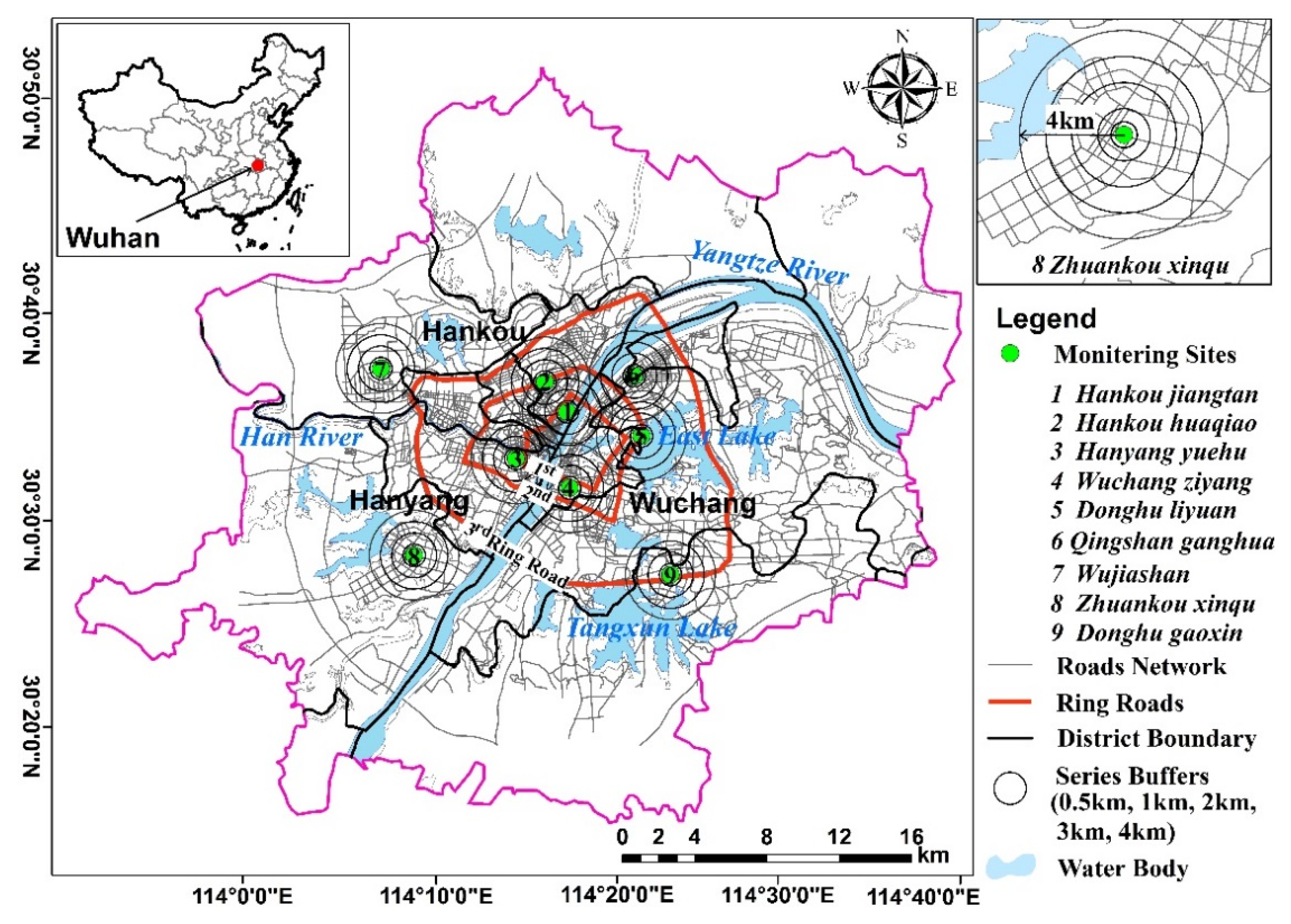
2.1. Research Area

Wuhan, the capital city of Hubei Province, is one of the largest cities in Central China and is located in the northeast of Jianghan Plain between 113°41′–115°05′ E and 29°58′–31°22′ N (Figure 1). Wuhan is currently a very important regional traffic hub of China. The Yangtze River and Han River join together in urban areas of Wuhan, dividing it into three parts, Hankou, Wuchang and Hanyang. There are 13 districts in Wuhan city with a total area of 8494 km2, seven of which make up central urban area and the other six districts are regarded as suburban areas. There are three ring roads in Wuhan city, which comprise the skeleton of urban structure (Figure 1). It is urban core area within the first ring road that is also called inner ring road. The second ring road with a total length of 48 km is the express way around the central urban area. The third ring road in Wuhan city is nearly the dividing line of urban and suburban area. Water bodies cover a quarter of the entire territory of Wuhan [36]. Tangxun Lake (48 km2), located in the northeast of the urban area, is the largest inner-city lake in Asia, and other main lakes include East Lake (33 km2), Sha Lake, South Lake and so on.
Wuhan is undergoing rapid industrialization and urbanization in the past decades [37,38,39]. In 2014, more than 10 million people live in this city with a total GDP exceeding 1 trillion RMB (approximately 154 billion US dollars) [40]. Population and business enterprises increase with the fast rate of urbanization, while the urban size also expands constantly and results in rapid urban land use change. According to statistics, the built-up area of Wuhan expanded more than 300 km2 from 2000 to 2014 with an annual average rate of 12% [40]. In contrast to the constant growth of the built-up area, water bodies in Wuhan shrank from 140 km2 (1995) to 90 km2 (2010) [38]. The boundary in magenta color shown in Figure 1 is the extent of Wuhan metropolitan area where central urban area (seven districts) and some part of suburban area are included with a planning area over 3000 km2, according to the general urban plan of Wuhan city (2010–2020).

2.2. Data Acquisition

2.2.1. Ambient Air Quality

As a vital industrial base in Central China, Wuhan experiences huge industrial emission and consumes massive volumes of energy. It is also an inland city with a poor meteorological situation for air circulation and diffusion, which makes the air pollution very serious all of the time. Automatic monitoring of ambient air quality in Wuhan city can retrospect to the 1980s. Air pollutants considered in the monitoring system have also changed with the variation of air pollution. For instance, nitrogen oxides (NOx) and total suspended particles (TSP) have been replaced since 2001 by NO2 and PM10, respectively. Fine particulate matter (PM2.5) has been added in the new ambient air quality standards (GB 3095-2012) [41] and has been monitored routinely since 2013. Currently, there are nine national-control monitoring sites in urban areas of Wuhan displayed in Figure 1. The detailed information on monitoring sites is shown in Table S1.
Although NO2 and PM10 have been monitored since 2001, the annual mean concentration specifying at each monitoring site before 2007 is not publicly available. In this study, the annual concentrations of SO2, NO2 and PM10 measured from 2007 to 2014 at the nine monitoring sites are used, which is available at the Wuhan Environmental Quality Communique [42].

2.2.2. Land Use Information

Landsat series images are used for land use information acquisition through image interpretation in each year from 2007 to 2014. In this study, we focus on the impacts of three land use categories, namely, built-up land, water bodies and vegetation, on air quality. To acquire land use information more objectively, we chose two Landsat images taken on different dates in each year. Images taken in the summer time are used as priorities for time consistency and also for the convenience and accuracy of vegetation information interpretation. However, farmland in summer around the suburban area (mainly at Site 7) is confused with vegetation. Compared to natural vegetation such as forest in urban area, farmland may have different effect on air quality since farmland in fallow is one of the sources of coarse particles due to the suspension of soil dust. Therefore, farmland is also classified in image interpretation, but its impacts on air quality will not be analyzed here because there is no farmland in the urban area. Those images covering Wuhan city (Path: 123, Row: 39) are downloaded from the Geospatial Data Cloud [43]. For the years of 2013 and 2014, Landsat-8 OLI images are chosen. For the years before 2013, Landsat-5 TM images are chosen because the sensor aboard the Landsat-7 satellite was broken, which resulted in stripes on the images since 2003. The Landsat-5 TM images available are all influenced by heavy cloud cover in the summer of 2010 and 2012; therefore, we have chosen appropriate Landsat-7 ETM images. Only one suitable Landsat-7 ETM image is chosen for the year of 2012, while there are two images for all of the other years, with 15 images in total. Stripes on Landsat-7 ETM images is repaired using multiple images and a self-adaptive regression model on the Geospatial Data Cloud. Detailed information on those 15 images is shown in Table S2.
Most of the selected images are cloud-free or have very little cloud cover (<4%). Although there is more than 10% cloud cover from images taken in 2008 (17 July), 2009 (20 July) and 2014 (22 October), our study area is not clouded because the research area only occupies small parts of the whole image. Radiation and geometrical correction of images had been carried out before we downloaded the images and those covering the Wuhan metropolitan area were cut out using vector edge in ENVI5.0 (ESRI). Four types of training samples (region of interest, ROI), built-up land, water bodies, vegetation and farmland, were depicted in ENVI5.0 whose number for each type is more than 50. The supervised classification method (maximum likelihood) was used for image classification if each ROI separability exceeded 1.8. Accuracy evaluation of image classification mainly relied on additional independent samples (more than 50 samples for each type of ROI) and Google high spatial-resolution images were also used to acquire ancillary information. Images were revised or reclassified according to the results of accuracy assessment and, finally, the overall accuracy of each image is higher than 90%.

2.2.3. Other Factors Influence Air Quality

Other factors that may influence air quality should be taken into consideration when analyzing the impacts of land use on air quality [20]. The concentrations of air pollutants and their spatial distribution are mainly influenced by their sources and the meteorological conditions [44]. Source apportionment of air pollutants indicates that industry emissions, vehicle exhaust, coal burning and construction dust are the foremost sources of urban air pollution in Wuhan city [45]. We select variables from five aspects (factors), namely, socio-economic development, energy use, traffic emission, industrial emission and meteorological condition, to control the influences of other factors on air quality (Table 1).

Socio-economic Development and Energy Use

The socio-economic development index includes residential population and gross domestic product (GDP) at the end of each year (2007–2014). For energy use, volumes of energy consumption by enterprises above the designated size (referring to more than 20 million RMB of income each year for the main business) and energy consumption per unit of GDP (energy efficiency) are collected at the end of each year (2007–2014). However, it is difficult to collect specific data at monitoring sites, for variables of socio-economic development and energy use, statistical data on a district where one site is located is used to represent the value of the corresponding site.

Traffic Emission

It is challenging to acquire detailed traffic emission or traffic volume data at each site among different years. We assume that more motor vehicles will travel around those sites with higher density of road network, correspondingly, bringing about more traffic emission. Under that assumption, the density of the road network (road length within buffers) around site is used to represent traffic emission. The road network includes arterial road, secondary trunk road and branch road, which comprise the public transport system in Wuhan city, but internal road within residential area is not included. However, only vector road network of Wuhan city in 2014, which is editable in GIS software, is collected. Among the series buffers with five different radiuses (Figure 1), road length within 2-km buffer around the site shows the highest average correlation coefficient with the concentrations of three air pollutants in 2014. Since fast urbanization in Wuhan city would cause remarkable change of roads, based on road length within 2-km buffer around sites in 2014, traffic emission around sites in other years will be modified by the numbers of registered motor vehicles in each year and it will be calculated using Formula (1):
R d _ d e n s i , t = V e h i _ n u m b t V e h i _ n u m b 2014 R d _ d e n s i , 2014
where Rd_densi,t represents the road length within 2-km buffer of the site i in the year t, i~(1–9), t~(2007–2014); Rd_densi,2014 represents the road length within 2-km buffer of the site i in 2014; Vehi_numbt represents the number of registered motor vehicles in the year t for the whole city; and Vehi_numb2014 represents the number of registered motor vehicles in 2014, which is the highest number (1.82 million) in 2007–2014.

Industry Emission

As for industry emission, we collected industrial waste gas emission for each year in 2007–2014 for the whole city, which contains SO2 emission, NOx emission, smoke powder emission, and other gaseous pollutants. We have no access to industrial emission data at sites or districts, but the numbers of enterprises above the designated size (referring to more than 20 million RMB of income each year for the main business) in each district are available. For a certain year, industrial emission data for the whole city will be apportioned to the districts by the numbers of enterprises of each district. The industry emission of each district will be used to represent the industry emission around sites according to which districts sites are located at. Industrial emission around each site for each year is calculated using Formula (2):
I n d u _ e m i s i , t = N i , t S u m t T o t a l _ e m i s t
where Indu_emisi,t represents industry emission of the site i in the year t, i~(1–9), t~(2007–2014); Total_emist represents the industry emission of the whole city in the year t; Ni,t represents number of enterprises above the designated size in the year t of the district where site i is located, and Sumt represents the total numbers of enterprises above the designated size in the year t for the whole city.

Meteorological Condition

Two meteorological parameters, the annual averages of temperature and precipitation in 2007–2014, are collected from one meteorology station located in the study area. Because we are currently focusing on the long-term variation of air quality and wish to avoid the effects of extreme precipitation, the number of days with precipitation greater than or equal to 0.1 mm, rather than the total precipitation throughout a year, is adopted to indicate the influences of precipitation on air quality. Meteorology data is used here for partially explain inter-annual variation of air pollutants. Since annual meteorological conditions show little variation within a city, they will be the same for nine sites for a certain year in the following modeling.

2.3. Methods

2.3.1. Buffer Analysis

The spatio-temporal response of the air quality at monitoring sites to land use varies by spatial scales. Series buffers are created at each monitoring site in ArcGIS10.1 (ESRI) to acquire land use variables of diverse spatial scales (Figure 1). The average distance from those sites inside the third ring road to theirs nearest site is 4.7 km and there is only 1.8 km from Site 1 (Hankou jiangtan) to Site 2 (Hankou huaqiao), which is the nearest between any two sites. Differences of land use categories around monitoring sites will not be distinguished evidently if the radius of buffer is too large. In our study, we set five buffers with radiuses as 0.5, 1, 2, 3, 4 km (Figure 1). For a given year, areas of three land use categories within each buffer are calculated and they are termed as land use variables (e.g., for year of 2007, area of built-up land within 1 km buffer is termed as Built-up land_1km_2007). Land use variables for each year are averages from two images excluding the year of 2012.

2.3.2. Correlation Analysis and Regression Modeling

Land use variables at the nine monitoring sites over eight years are organized with the concentrations of air pollutants resulting in a dataset with 72 records in total. Using bivariate correlation analysis in SPSS21.0 (IBM), we want to identify the magnitude of correlation between land use categories and air pollutants at varying spatial scales (radiuses). The optimum correlation scale between a certain land use category and a certain air pollutant is defined as the radius with the highest correlation coefficient between them. Since concentrations of air pollutants and most land use variables are normal distribution (Figure S1), Pearson’s correlation coefficient is used in correlation analysis like related studies [46]. After identifying the optimum correlation radiuses, quantitative effects of land use on air quality will be modeled using a stepwise linear regression model combining other independent variables as previous studies [47,48]. In this study, a bidirectional elimination stepwise linear regression model will be developed for each air pollutant. With regard to the impact of the same land use category on a certain air pollutant, only land use variable under the optimum radius will be considered in the regression modelling because land use variable with the optimum radius has higher explanatory ability for the variability of air quality than variables under other spatial scales (radiuses). All of the independent variables considered in quantitative modelling are shown in Table 1.

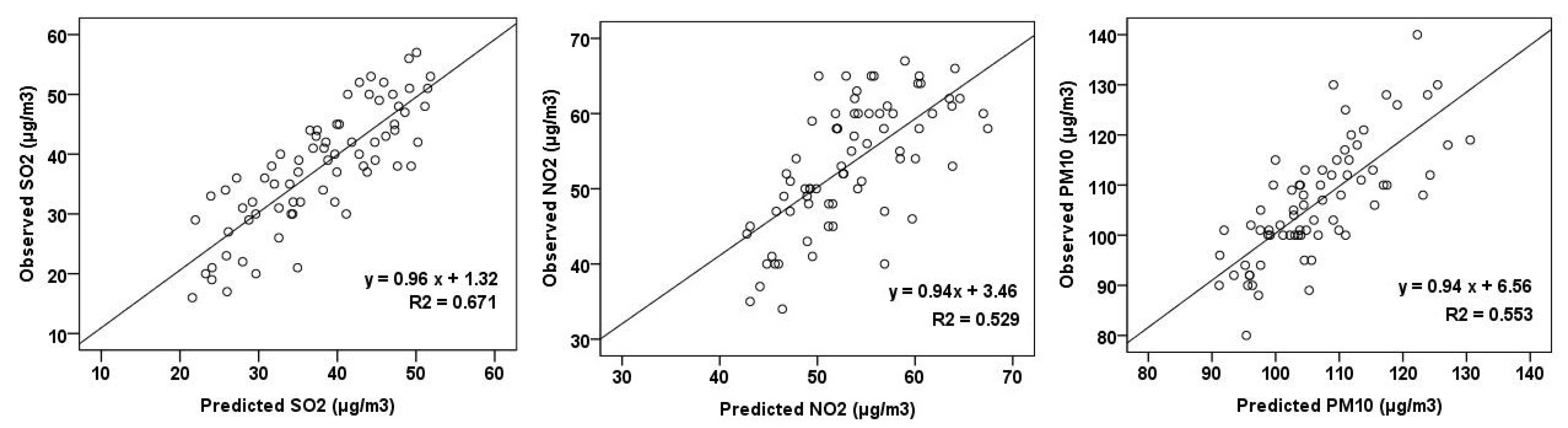
2.3.3. Cross Validation

In order to validate the performance of the regression models, the leave-one-out-cross-validation (LOOCV) technique is adopted. The LOOCV has been widely used in related studies [33]. In this study, the regression model, with the same independent variables as the outcome of stepwise linear regression, is developed for n1 sites and the predicted concentrations are compared with the actually observed concentrations at the left-out site. The process is repeated n times so that each site is left out once. The measure of performance in the LOOCV procedure is the R2 parameter estimated for the fit between the observed and predicted concentrations of air pollutants. The LOOCV technique will be executed three times for the regression models of SO2, NO2 and PM10, respectively.

3. Results

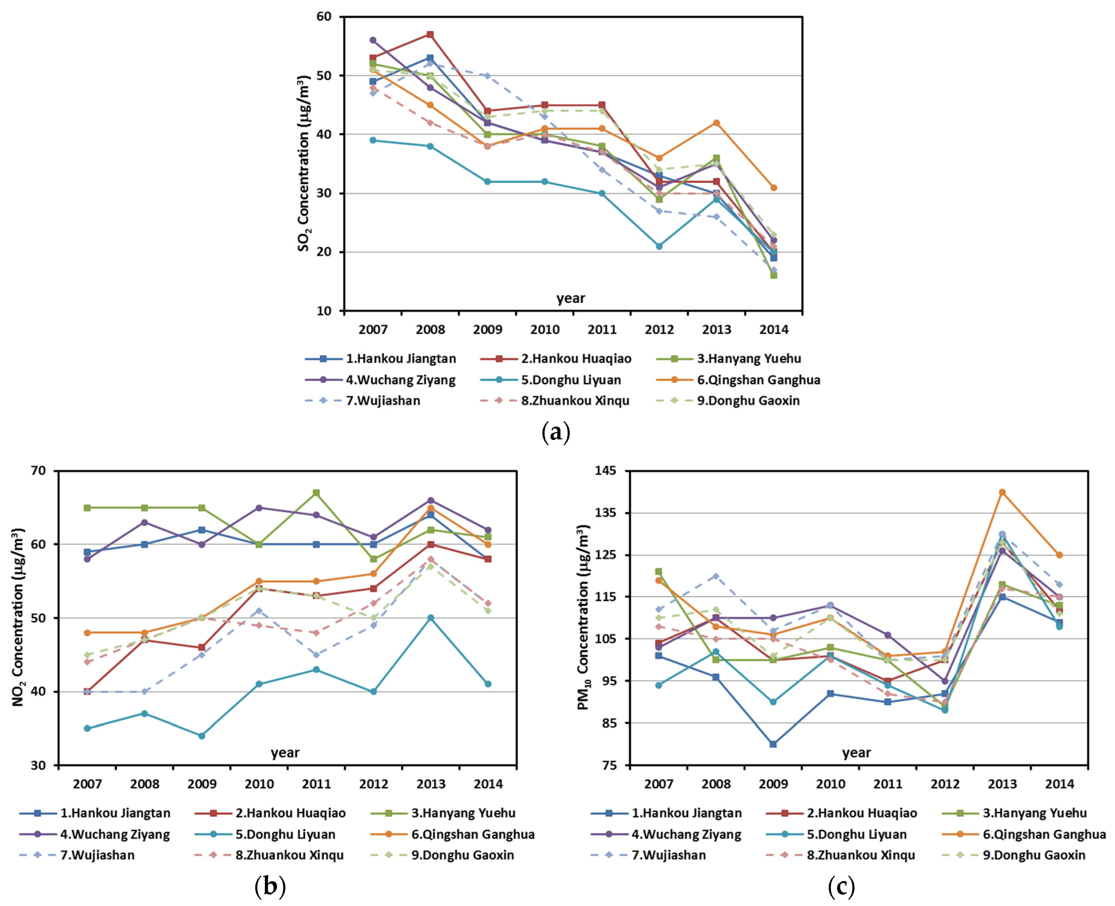
3.1. Spatio-Temporal Variation of Air Pollutants

Inter-annual variation of concentrations of three different air pollutants in the Wuhan urban area, summarized from the nine monitoring sites, are shown as Figure 2 with the error bars representing the standard deviation of concentrations.
Different variation tendencies of air pollutants can be seen from Figure 2 during the research period. There is a dramatic increase in the PM10 concentration in 2013 after a continuous decrease in the preceding years, while a stable rising trend for NO2 concentration can also be detected; however, the SO2 concentration declines from the beginning to the end. According to the China National Ambient Air Quality Standard (NAAQS, GB 3095-1996) [49], annual average Level-2 limitations for SO2, NO2, and PM10 are 60, 40, 100 μg/m3, respectively. In 2012, China enacted a new Ambient Air Quality Standard (NAAQS, GB 3095-2012) [41] that replaced the previous one. Although Level-2 limitations for SO2 and NO2 stay the same, the limitation for the PM10 annual average concentration has been down-regulated to 70 μg/m3.
The only one meeting the requirement of the new standard is SO2 concentration. SO2 pollution in Wuhan has been effectively controlled over recent years owing to rigorous environmental policy and management. However, with rapid urbanization, the increased volume of motor vehicles and sprawl of construction sites, pollution of nitrogen oxides and particulate matter are still at a very high level [45,50,51]. It is clear that there is a very long way to go for PM10 attainment according to the new Ambient Air Quality Standard; additionally, the nonattainment of NO2 concentrations persists throughout the study. Previous studies demonstrate that motor vehicle exhaust is the main source of urban air pollution, especially for NOx and particles [52]. The volume of motor vehicles in Wuhan city has increased from 0.76 million in 2007 to 1.82 million by the end of 2014 [40]. Additionally, this number has been increasing by more than 0.2 million vehicles every year in the most recent three years. The rapid increase of motor vehicles is responsible for continuous high level NO2 pollution and PM pollution.
Inter-annual variations of concentrations of SO2, NO2 and PM10 from 2007 to 2014 at each site are shown in Figure 3, in which the spatial variability of air pollution among different sites can be identified as well. The spatial distributions of eight-year (2007–2014) average concentrations of SO2, NO2 and PM10 are simulated using IDW interpolation with a searching radius of 7.9 km in ArcGIS10.1 (ESRI) and the results are shown in Figure S2. The methodology of IDW interpolation can be found in other publications in detail [53,54].
Spatial disparity of the NO2 pollution is the most obvious observation because NO2 concentrations at Site 1 (Hankou jiangtan), Site 3 (Hanyang yuehu) and Site 4 (Wuchang ziyang) have been constantly maintained a high level (Figure 3) that is significantly higher than the other sites. Average NO2 concentration (61.9 μg/m3) at those three sites in eight years is 1.5 times higher than their counterpart at Site 5 (Donghu liyuan) (40.1 μg/m3), whose NO2 concentration is the lowest. As shown in Figure 1, those three sites are located around the first ring road in the urban core with a dense population and massive volumes of traffic, which accounts for the much more severe NO2 pollution than the other sites.
As for the variation of pollution level, all three air pollutions at Site 6 (Qingshan ganghua) became even worse relative to the pollution level of other sites, especially for SO2 and PM10 concentration. For the past few years, energy-intensive and highly polluted enterprises have been gradually removed from the urban core to suburban areas with the implementation of industrial policy in Wuhan. Consequently, many heavy industry enterprises gathered in the Qingshan district in the northeast of Wuhan, which made the air quality gradually worse.
By contrast, air quality at some other sites is improving. For instance, the SO2 concentration (52 μg/m3) and PM10 concentration (121 μg/m3) at Site 3 (Hanyang yuehu) in 2007 are the third and first highest levels among the nine sites, respectively. Conversely, in 2014, the site is ranked among the lowest for these pollution levels. Located around Site 3 (Hanyang yuehu), the QinTai Grand Theatre, which covers an area of 2.5 hectares, was under construction in 2004–2007 (started in May 2004, finished in August 2007). Construction dust and large-scale machinery operation worsened the SO2 and PM10 pollution levels. Landscapes were remediated shortly after this vast building was completed; correspondingly, the air quality here has been improved, and this area, called Moon Park, is now one of the most famous cultural entertainments in Wuhan city. Compared with the decreasing SO2 and PM10 pollution level, Site 3 has been suffering from severe NO2 pollution throughout the study period. Site 3 is near the approach bridge to the Wuhan Yangtze River Bridge, which is the first bridge built over the river. There is an average of 100,000 vehicles that cross this bridge (two-way) every day; therefore, huge vehicle exhaust is an important reason for severe NO2 pollution at Site 3. There is also an obvious improvement in SO2 pollution at Site 1 (Hankou jiangtan) and Site 7 (Wujiashan). All three types of pollutant concentrations at Site 5 (Donghu liyuan), located in the national 5A-level East Lake Scenic Area, are at a relatively low level.

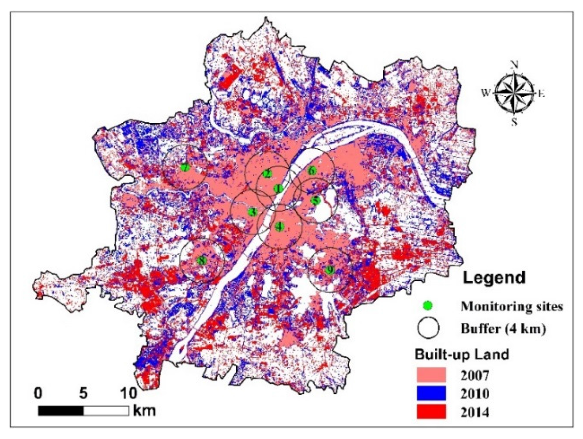
3.2. Land Use Pattern and Change

Tremendous urban land use change occurs under the process of rapid urbanization, especially for the rapid expansion of built-up land. Wuhan has been experiencing rapid urban expansion from 2007 to 2014, especially for the East Lake High-Tech Industrial Development Zone located in the southeast of Wuhan and the Zhuankou Economic and Technological Development Zone located in the southwest of Wuhan (Figure 4).
Areas of land use categories within a 4-km buffer are calculated for each year to quantify the land use pattern and changes around the monitoring sites. Of course, there is a difference in land use between the 4-km buffer and others. The averaged proportions of land use categories at each site in the first four years (2007–2010) and the last four years (2011–2014) are shown in Table 2.
It can be seen from Table 2 that the proportion of land use categories among these sites varies greatly. As for the proportions at each site in the first four years (2007–2010): (1) the average proportion of built-up land at those sites located in urban core (Hankou jiangtan, Hankou huaqiao, Hanyang yuehu, Wuchang ziyang) is nearly up to 80%, with the built-up land proportion at Site 2 (Hankou huaqiao) being approximately 90%, while average proportion of vegetation is less than 5% at those sites; (2) the average proportion of built-up land at those sites located in urban periphery (Qingshan ganghua, Wujiashan, Zhuankou xinqu, Donghu gaoxin) is no more than 65%, while the average proportion of vegetation is nearly up to 20% at those sites, with the proportion of vegetation at Site 7 (Wujiashan) being approximately 35%; and (3) the areas of water bodies vary significantly among the nine sites with the highest proportion exceeding 40% at Site 5 (Donghu Liyuan) where exists the minimum proportion of built-up land (47.4%). Different proportions of land use categories around these sites will have differing impacts on their air quality.
As for land use change, the area change in built-up land within a 4-km buffer at each site is different while areas of water bodies and vegetation decline and increase, respectively, at most sites. On average, areas of built-up land and vegetation at the nine sites in the last four years increase by 0.1% and 0.7%, respectively, compared with the first four years, whereas the corresponding areas of water bodies decrease by 0.8%. There is little land use change if we take a holistic view, however, obvious differences in land use change exist at each site. (1) Areas of built-up land and vegetation at those sites located in the urban core (Hankou Jiangtan, Hankou Huaqiao, Hanyang Yuehu, Wuchang Ziyang) on average decrease by 2.6% and increase by 3.3%, respectively, owing to the implementation of plant engineering in the urban area; (2) Extensive urban expansion occurs at those sites (Wujiashan, Zhuankou xinqu, Donghu gaoxin) in urban periphery, which accounts for the maximum increase in built-up land (5.5%) at Site 7 (Wujiashan). The rising of built-up land at Site 7 (Wujiashan) and Site 9 (Donghu gaoxin) mainly comes from the decrease in vegetation, while the water bodies reduction contributes mostly to the increase in built-up land at Site 8 (Zhuankou xinqu); (3) There is also a 1% reduction of built-up land at Site 6 (Qingshan Ganghua) where urban construction activities were carried out very early. Additionally, built-up land at Site 5 (Donghu liyuan), which is located in the urban core, increases due to land development and construction around the area in recent years.

3.3. Correlation Analysis between Land Use Variables and Air Pollutants

Correlation analysis between land use variables and air pollutants is the foundation to identify their interrelated magnitude and optimum radius. The results of the bivariate correlation analysis are shown as Table 3.
As shown in Table 3, at least three aspects of land use impacts on the air quality can be concluded. (1) Positive or negative correlation between land use categories and the same kind of air pollutant depends on different land use categories. For instance, built-up land has a positive correlation with all three types of air pollutants, while water bodies and vegetation have negative correlation with all three types of air pollutants; (2) There is an obvious spatial scale effect for the magnitude of correlation between land use and air quality. For example, built-up land within a 0.5-km buffer is not significantly associated with NO2 concentration, whereas the correlation coefficients (Pearson’s r) between the built-up land within the 2 km, 3 km and 4 km buffer and NO2 concentration are 0.347, 0.374 and 0.411, respectively, and all are statistically significant (p < 0.01); (3) The same land use category shows various magnitude of correlation with different air pollutants. For instance, the highest correlation coefficient between built-up land and NO2 concentration reaches at 0.411, while it is only 0.280 and 0.219 for SO2 and PM10 concentration, respectively. Similarly, absolute value of the highest correlation coefficient between water bodies and PM10 concentration (−0.401) is higher than values for SO2 and NO2 concentration.
The radius with the highest Pearson’s r between land use category and air pollutant is considered as the optimum radius. The optimum correlation radius between land use variables and air pollutants is shown in boldface in Table 3. It shows that the optimum correlation radius between water bodies or vegetation and air pollutants varies from 1 to 2 km. However, there is a great difference in the optimum radiuses for impacts of built-up land concerning different air pollutants. From the perspective of air pollutants, optimum radiuses between different land use categories and SO2 and PM10 are relatively smaller, whereas that for NO2 is relatively larger. This is likely because SO2 and PM10 emissions are mainly from point sources, while non-point emission mostly contributes to the NO2 concentration.

3.4. Quantitative Effects of Land Use on Air Quality

Taking the annual average concentration of air pollutants as dependent variables and all influence factors, including land use variables, as independent variables (Table 1), stepwise linear regressions (bidirectional elimination) are used for modeling the quantitative impacts of land use on air quality. Regression model has been developed for each air pollutant. As mentioned in Section 2.3.2, only land use categories under the optimum radiuses will be used in regression models. For instance, only area of built-up land within 1-km buffer is used in SO2 regression model to quantify the impacts of built-up land on SO2 pollution and areas of built-up land within other buffers will not be used because the optimum correlation radius between built-up land and SO2 concentration is 1 km (Table 3). Land use variables for the same land use category (e.g., built-up land) may have different radiuses in different air pollutants’ regression models. The standardized coefficients of regressions for different air pollutants are summarized in Table 4 and the results of leave-one-out-cross-validation (LOOCV) are shown in Figure 5.
All three stepwise linear regression models are statistically significant (p < 0.001) with high fitting precision. The adjusted R-square value of each regression model varies from 0.575 to 0.696 and the R-square value of cross validation results is a little lower, varying in 0.529–0.671 (Figure 5). In terms of particular air pollutant, the independent variables in the final regression model are different. For instance, five independent variables are included in the final regression model for SO2 concentration (column (1)), which are water bodies, GDP, energy efficiency, industrial waste gas emission, and precipitation. There are five independent variables in PM10 regression model as well (column (2)), while only four independent variables are included in NO2 regression model (column (3)). Positive or negative coefficients of the majority variables in the regression models (Table 4) are easy to understand. The coefficients of build-up land, energy use and road density in regression models are positive and the coefficients of water bodies, vegetation and precipitation are negative. However, the coefficient of industrial waste emission in SO2 regression model is negative, which may not meet our expectations. In fact, industrial waste emission increases from 300 billion to nearly 600 billion standard cubic meters in 2007–2014 for the whole city, while SO2 concentration decreases from 50 to 21 μg/m3 during the same period. Actually, industrial waste emission is negatively correlated with SO2 concentration (Pearson’s r = −0.307, p < 0.01) and this relationship may cause the negative coefficient in the final regression model. This undesirable result may also associated with our coarse apportionment method for industrial emission. The coefficient of GDP in SO2 regression model is negative but in PM10 regression model, it is positive. One reasonable explanation is that SO2 and PM10 pollution is in the different stage of the environmental Kuznets curve (EKC), which suggests that rising income increases pollution when GDP is low, but decreases pollution when GDP is high [55,56].
Focusing on land use variables, water bodies show significantly negative effects in SO2 and PM10 regression models and built-up land contributes to NO2 pollution considerably, while for vegetation, it is only included in NO2 regression model. Percent changes in air quality (compared to the mean value) associated with every one standard deviation increase from mean value of each independent variable are presented in Figure 6, while all other independent variables are held at mean value. The influence magnitude of independent variables on air pollutants can also be compared by their standardized coefficients in the models. In SO2 regression model, the impact of one standard deviation increase of energy efficiency (energy consumption per unit of GDP, 5.8%, p < 0.01) can be offset by the mitigation effect of one standard deviation increase of water bodies within 1-km buffer (−5.8%, p < 0.01) and the mitigation effect of water bodies is comparable to the effects of precipitation (−8.1%, p < 0.01). Road density has the highest standardized coefficient (0.586, p < 0.01) in NO2 model that shows the strong impacts of traffic emission on NO2 pollution. Built-up land and vegetation also have significant impacts on NO2 pollution. Built-up land with one standard deviation increase will cause 1.6% (p < 0.05) increases in NO2 concentration while increases of water bodies with one standard deviation will decrease 5.0% (p < 0.01) of NO2 concentration. PM10 concentration is mainly influenced by energy use and industrial emission, however, water bodies also show significant mitigation effect (−3.3%, p < 0.01).

4. Discussion

The biggest challenge of quantitatively modeling the relationship between land use and air quality in this study is the sparse ambient air quality monitoring sites. In order to improve the robustness of regression modeling limited by the sparse sites, the geographic environments and air quality at nine sites over eight years (2007–2014) are organized in a dataset with 72 records. However, the identified association between them could be confounded by the temporal trend of air quality and geographic environments in this way. Another difficulty is the limitations of data accessibility of other independent variables at each site. The data for socio-economic development, energy use and industry emission is at district level, which is different from air quality data at sites. Some variables are replaced due to data limitations, for example, road length within buffers modified by the number of registered motor vehicles is used as a proxy. The appropriate variable for traffic emission or volume is VKT (vehicle kilometers of travel) in each cell, which has been widely used in developed countries [57]. In addition, only the numbers of enterprises above the designated size are taken into consideration when the total emission are apportioned to each districts thus the huge disparity of industrial emission of different types of enterprises cannot be distinguished. All of those may affect the results of quantitatively modeling the impacts of land use on air quality.
With regard to the modeling approach, the air quality and geographic environments are arranged with the same year in this study. However, the change in geographic environments could take some time to result in air quality changes. Although annual average concentrations of air quality are used which are the aggregated impacts of geographic environments for one year, the time lagged effect of geographic environments on air quality may affect the association between them, which can be studied in further research. Stepwise linear regression (bidirectional elimination) is used to quantitatively model the impacts of land use on air quality in our study as used in other related researches [47]. New independent variables are accepted in the model if they are statistically significant (p < 0.1). As a result, all independent variables in the final stepwise linear regression model are statistically significant thus the multicollinearity among variables is reduced [47]. However, some variables that we are concerned about may be removed in the process of stepwise modeling. For instance, areas of built-up land within certain buffers are significantly correlated with SO2 concentration (r = 0.280, p < 0.05, see Table 3) and PM10 concentration (r = 0.219, p < 0.10, see Table 3), but built-up land variables are not included in the final regression models of SO2 and PM10. In addition, other factors influencing air quality like regional transport of air pollutants are not taken into account in our study and it may increase uncertainty of the final regression models.

5. Conclusions

Urban air quality has been deteriorating gradually by the rapid urban land use change in line with the city growth. This study contributes to research on air quality and land use by examining the quantitative relationship specified at ground-level monitoring sites from a long-term (2007–2014) spatial and temporal perspective. Land use categories have discriminatory effects on different air pollutants, whether for the direction of correlation, magnitude of correlation or spatial scales effect of correlation. Areas of built-up land are positively correlated with concentrations of all three pollutants (SO2, NO2, and PM10) with the strongest relationship with NO2 concentration (r = 0.4). Water bodies show significant mitigation effect for SO2 and PM10 pollution in the final regression models. The impacts of water bodies are comparative to the effects of meteorology factors (precipitation), which are widely considered to be important for air quality. The relationship between land use variables and air quality identified here is also beneficial for the model to simulate the spatial distribution of air pollutants combining land use information, such as the land use regression (LUR) model.
Urban developments and land use patterns have profound impacts on urban air quality not only by influencing the volume of emissions but also by affecting the ability of the urban ecosystem to purify the air. However, it is not so easy to quantitatively model the relationship between land use and air quality because it varies at time and space and is influenced by many other geographic environments. More detailed and comprehensive data is needed, especially in ground-level air quality data and traffic volume data such as VKT information, which could be an area of further research in China. Air quality improvement is a long process and air pollution problem could not be solved thoroughly only relying on emission control or technology advancement. Urban developments and land use patterns should be paid much attention. It is necessary to develop sustainable urban land use policies to control and reduce air pollution without limiting economic growth. Government policy and public action for air pollution reduction could refer to land use strategies apart from other pollution reduction mechanisms.

Supplementary Materials

The following are available online at www.mdpi.com/2073-4433/7/5/62/s1. Figure S1: Frequency distribution histograms of air pollutants and land use variables, Figure S2: Spatial distribution of eight-year (2007–2014) average concentrations of three air pollutants in Wuhan based on IDW interpolation in ArcGIS10.1 with default parameters: (a) SO2 concentration; (b) NO2 concentration; (c) PM10 concentration, Table S1: Detailed description of nine ambient air quality monitoring sites in Wuhan, Table S2: Detailed information on satellite images used for land use information acquisition.

Acknowledgments

This study was funded by the National Natural Science Foundation of China (No. 41571385).

Author Contributions

Limin Jiao and Gang Xu conceived and designed the experiments; Gang Xu, Suli Zhao, Man Yuan and Xiaoming Li performed the experiments under the guidance by Limin Jiao; Yuyao Han, Boen Zhang, and Ting Dong collected and processed the data; Gang Xu wrote the paper.

Conflicts of Interest

The authors declare no conflict of interest.

References

  1. Foley, J.A. Global Consequences of Land Use. Science 2005, 309, 570–574. [Google Scholar] [CrossRef] [PubMed]
  2. Seto, K.C.; Fragkias, M.; Gueneralp, B.; Reilly, M.K. A Meta-Analysis of Global Urban Land Expansion. PLoS ONE 2011, 6, e23777. [Google Scholar] [CrossRef] [PubMed]
  3. Jiao, L. Urban land density function: A new method to characterize urban expansion. Landsc. Urban Plan 2015, 139, 26–39. [Google Scholar] [CrossRef]
  4. Grimm, N.B.; Faeth, S.H.; Golubiewski, N.E.; Redman, C.L.; Wu, J.; Bai, X.; Briggs, J.M. Global Change and the Ecology of Cities. Science 2008, 319, 756–760. [Google Scholar] [CrossRef] [PubMed]
  5. Duh, J.; Shandas, V.; Chang, H.; George, L.A. Rates of urbanisation and the resiliency of air and water quality. Sci. Total Environ. 2008, 400, 238–256. [Google Scholar] [CrossRef] [PubMed]
  6. Heald, C.L.; Spracklen, D.V. Land Use Change Impacts on Air Quality and Climate. Chem. Rev. 2015, 115, 4476–4496. [Google Scholar] [CrossRef] [PubMed]
  7. Turner, B.L.I.; Lambin, E.F.; Reenberg, A. The emergence of land change science for global environmental change and sustainability. Proc. Natl. Acad. Sci. U.S.A. 2007, 104, 20666–20671. [Google Scholar] [CrossRef] [PubMed]
  8. Jiang, Y.; Fu, P.; Weng, Q. Assessing the Impacts of Urbanization-Associated Land Use/Cover Change on Land Surface Temperature and Surface Moisture: A Case Study in the Midwestern United States. Remote Sens. 2015, 7, 4880–4898. [Google Scholar] [CrossRef]
  9. Yan, Y.; Zhang, C.; Hu, Y.; Kuang, W. Urban Land-Cover Change and Its Impact on the Ecosystem Carbon Storage in a Dryland City. Remote Sens. 2016, 8, 6. [Google Scholar] [CrossRef]
  10. Song, J.; Webb, A.; Parmenter, B.; Allen, D.T.; McDonald-Buller, E. The Impacts of Urbanization on Emissions and Air Quality: Comparison of Four Visions of Austin, Texas. Environ. Sci. Technol. 2008, 42, 7294–7300. [Google Scholar] [CrossRef] [PubMed]
  11. Chen, B.; Yang, S.; Xu, X.; Zhang, W. The impacts of urbanization on air quality over the Pearl River Delta in winter: Roles of urban land use and emission distribution. Theor. Appl. Climatol. 2014, 117, 29–39. [Google Scholar] [CrossRef]
  12. Fang, C.; Liu, H.; Li, G.; Sun, D.; Miao, Z. Estimating the Impact of Urbanization on Air Quality in China Using Spatial Regression Models. Sustainability 2015, 7, 15570–15592. [Google Scholar] [CrossRef]
  13. Tecer, L.H.; Tagil, S. Impact of Urbanization on Local Air Quality: Differences in Urban and Rural Areas of Balikesir, Turkey. Clean Soil Air Water 2014, 42, 1489–1499. [Google Scholar] [CrossRef]
  14. Chan, C.K.; Yao, X. Air pollution in mega cities in China. Atmos. Environ. 2008, 42, 1–42. [Google Scholar] [CrossRef]
  15. Fenger, J. Air pollution in the last 50 years—From local to global. Atmos. Environ. 2009, 43, 13–22. [Google Scholar] [CrossRef]
  16. Guo, S.; Hu, M.; Zamora, M.L.; Peng, J.; Shang, D.; Zheng, J.; Du, Z.; Wu, Z.; Shao, M.; Zeng, L.; et al. Elucidating severe urban haze formation in China. Proc. Natl. Acad. Sci. U.S.A. 2014, 111, 17373–17378. [Google Scholar] [CrossRef] [PubMed]
  17. Romero, H.; Ihl, M.; Rivera, A.; Zalazar, P.; Azocar, P. Rapid urban growth, land-use changes and air pollution in Santiago, Chile. Atmos. Environ. 1999, 33, 4039–4047. [Google Scholar] [CrossRef]
  18. Weng, Q.; Yang, S. Urban Air Pollution Patterns, Land Use, and Thermal Landscape: An Examination of the Linkage Using GIS. Environ. Monit. Assess. 2006, 117, 463–489. [Google Scholar] [CrossRef] [PubMed]
  19. Xian, G. Analysis of impacts of urban land use and land cover on air quality in the Las Vegas region using remote sensing information and ground observations. Int. J. Remote Sens. 2007, 28, 5427–5445. [Google Scholar] [CrossRef]
  20. Superczynski, S.D.; Christopher, S.A. Exploring Land Use and Land Cover Effects on Air Quality in Central Alabama Using GIS and Remote Sensing. Remote Sens. 2011, 3, 2552–2567. [Google Scholar] [CrossRef]
  21. Huang, Y.; Luvsan, M.; Gombojav, E.; Ochir, C.; Bulgan, J.; Chan, C. Land use patterns and SO2 and NO2 pollution in Ulaanbaatar, Mongolia. Environ. Res. 2013, 124, 1–6. [Google Scholar] [CrossRef] [PubMed]
  22. Bandeira, J.M.; Coelho, M.C.; Sá, M.E.; Tavares, R.; Borrego, C. Impact of land use on urban mobility patterns, emissions and air quality in a Portuguese medium-sized city. Sci. Total. Environ. 2011, 409, 1154–1163. [Google Scholar] [CrossRef] [PubMed] [Green Version]
  23. Fameli, K.; Assimakopoulos, V.; Kotroni, V.; Retalis, A. Effect of the land use change characteristics on the air pollution patterns above the greater Athens area (GAA) after 2004. Glob. Nest J. 2013, 15, 169–177. [Google Scholar]
  24. Frank, L.D.; Sallis, J.F.; Conway, T.L.; Chapman, J.E.; Saelens, B.E.; Bachman, W. Many pathways from land use to health—Associations between neighborhood walkability and active transportation, body mass index, and air quality. J. Am. Plan. Assoc. 2006, 72, 75–87. [Google Scholar] [CrossRef]
  25. Jazcilevich, A.D.; Garc A, A.N.R.; Ru Z-Suárez, L.G. A modeling study of air pollution modulation through land-use change in the Valley of Mexico. Atmos. Environ. 2002, 36, 2297–2307. [Google Scholar] [CrossRef]
  26. Escobedo, F.J.; Nowak, D.J. Spatial heterogeneity and air pollution removal by an urban forest. Landsc. Urban Plan 2009, 90, 102–110. [Google Scholar] [CrossRef]
  27. Irga, P.J.; Burchett, M.D.; Torpy, F.R. Does urban forestry have a quantitative effect on ambient air quality in an urban environment? Atmos. Environ. 2015, 120, 173–181. [Google Scholar] [CrossRef]
  28. Du, N.; Ottens, H.; Sliuzas, R. Spatial impact of urban expansion on surface water bodies—A case study of Wuhan, China. Landsc. Urban Plan 2010, 94, 175–185. [Google Scholar] [CrossRef]
  29. Wilby, R.L. Constructing climate change scenarios of urban heat island intensity and air quality. Environ. Plan. B Plan. Des. 2008, 35, 902–919. [Google Scholar] [CrossRef]
  30. Sarrat, C.; Lemonsu, A.; Masson, V.; Guedalia, D. Impact of urban heat island on regional atmospheric pollution. Atmos. Environ. 2006, 40, 1743–1758. [Google Scholar] [CrossRef]
  31. Civerolo, K.; Hogrefe, C.; Lynn, B.; Rosenthal, J.; Ku, J.; Solecki, W.; Cox, J.; Small, C.; Rosenzweig, C.; Goldberg, R.; et al. Estimating the effects of increased urbanization on surface meteorology and ozone concentrations in the New York City metropolitan region. Atmos. Environ. 2007, 41, 1803–1818. [Google Scholar] [CrossRef]
  32. Shukla, V.; Parikh, K. The environmental consequences of urban growth: Cross-national perspective on economic development, air pollution, and city size. Urban Geogr. 1992, 13, 422–449. [Google Scholar] [CrossRef]
  33. Hoek, G.; Beelen, R.; de Hoogh, K.; Vienneau, D.; Gulliver, J.; Fischer, P.; Briggs, D. A review of land-use regression models to assess spatial variation of outdoor air pollution. Atmos. Environ. 2008, 42, 7561–7578. [Google Scholar] [CrossRef]
  34. Zou, B.; Luo, Y.; Wan, N.; Zheng, Z.; Sternberg, T.; Liao, Y. Performance comparison of LUR and OK in PM2.5 concentration mapping: A multidimensional perspective. Sci. Rep. 2015, 5, 8698. [Google Scholar] [CrossRef] [PubMed]
  35. Hennig, F.; Sugiri, D.; Tzivian, L.; Fuks, K.; Moebus, S.; Jöckel, K.; Vienneau, D.; Kuhlbusch, T.; de Hoogh, K.; Memmesheimer, M.; et al. Comparison of Land-Use Regression Modeling with Dispersion and Chemistry Transport Modeling to Assign Air Pollution Concentrations within the Ruhr Area. Atmosphere 2016, 7, 48. [Google Scholar] [CrossRef]
  36. Jiao, L.; Liu, Y. Geographic Field Model based hedonic valuation of urban open spaces in Wuhan, China. Landsc. Urban Plan 2010, 98, 47–55. [Google Scholar] [CrossRef]
  37. Jiao, L.; Mao, L.; Liu, Y. Multi-order Landscape Expansion Index: Characterizing urban expansion dynamics. Landsc. Urban Plan 2015, 137, 30–39. [Google Scholar] [CrossRef]
  38. Zeng, C.; Liu, Y.; Stein, A.; Jiao, L. Characterization and spatial modeling of urban sprawl in the Wuhan Metropolitan Area, China. Int. J. Appl. Earth Obs. 2015, 34, 10–24. [Google Scholar] [CrossRef]
  39. Tan, R.; Liu, Y.; Zhou, K.; Jiao, L.; Tang, W. A game-theory based agent-cellular model for use in urban growth simulation: A case study of the rapidly urbanizing Wuhan area of central China. Comput. Environ. Urban Syst. 2015, 49, 15–29. [Google Scholar] [CrossRef]
  40. Wuhan Bureau of Statistics. Wuhan Statistical Yearbook 2014; China Statistics Press: Beijing, China, 2014. [Google Scholar]
  41. MEP of China. Ambient Air Quality standard (GB 3095-2012); China Environmental Science Press: Beijing, China, 2012. [Google Scholar]
  42. Wuhan Environmental Monitoring Center. Available online: http://www.whemc.cn/news/hjzkgb/index.html (accessed on 16 October 2015).
  43. Geospatial Data Cloud. Available online: http://www.gscloud.cn (accessed on 27 September 2015).
  44. Gao, J.; Zha, Y. Meteorological Influence on Predicting Air Pollution from MODIS-Derived Aerosol Optical Thickness: A Case Study in Nanjing, China. Remote Sens. 2010, 2, 2136–2147. [Google Scholar] [CrossRef]
  45. Zhang, F.; Wang, Z.; Cheng, H.; Lv, X.; Gong, W.; Wang, X.; Zhang, G. Seasonal variations and chemical characteristics of PM2.5 in Wuhan, central China. Sci. Total Environ. 2015, 518–519, 97–105. [Google Scholar] [CrossRef] [PubMed]
  46. Chen, L.; Baili, Z.; Kong, S.; Han, B.; You, Y.; Ding, X.; Du, S.; Liu, A. A land use regression for predicting NO2 and PM10 concentrations in different seasons in Tianjin region, China. J. Environ. Sci. 2010, 22, 1364–1373. [Google Scholar] [CrossRef]
  47. Clark, L.P.; Millet, D.B.; Marshall, J.D. Air Quality and Urban Form in U.S. Urban Areas: Evidence from Regulatory Monitors. Environ. Sci. Technol. 2011, 45, 7028–7035. [Google Scholar] [CrossRef] [PubMed]
  48. Novotny, E.V.; Bechle, M.J.; Millet, D.B.; Marshall, J.D. National Satellite-Based Land-Use Regression: NO2 in the United States. Environ. Sci. Technol. 2011, 45, 4407–4414. [Google Scholar] [CrossRef] [PubMed]
  49. MEP of China. Ambient air quality standard (GB 3065-1996); China Environmental Science Press: Beijing, China, 1996. (In Chinese) [Google Scholar]
  50. Gong, W.; Zhang, T.; Zhu, Z.; Ma, Y.; Ma, X.; Wang, W. Characteristics of PM1.0, PM2.5, and PM10, and Their Relation to Black Carbon in Wuhan, Central China. Atmosphere 2015, 6, 1377–1387. [Google Scholar] [CrossRef]
  51. Feng, Q.; Wu, S.; Du, Y.; Li, X.; Ling, F.; Xue, H.; Cai, S. Variations of PM10 concentrations in Wuhan, China. Environ. Monit. Assess. 2011, 176, 259–271. [Google Scholar] [CrossRef] [PubMed]
  52. Westerdahl, D.; Wang, X.; Pan, X.; Zhang, K.M. Characterization of on-road vehicle emission factors and microenvironmental air quality in Beijing, China. Atmos. Environ. 2009, 43, 697–705. [Google Scholar] [CrossRef]
  53. Lu, G.Y.; Wong, D.W. An adaptive inverse-distance weighting spatial interpolation technique. Comput. Geosci. 2008, 34, 1044–1055. [Google Scholar] [CrossRef]
  54. Zhang, H.; Lu, L.; Liu, Y.; Liu, W. Spatial Sampling Strategies for the Effect of Interpolation Accuracy. ISPRS Int. J. Geo Inf. 2015, 4, 2742–2768. [Google Scholar] [CrossRef]
  55. Bechle, M.J.; Millet, D.B.; Marshall, J.D. Effects of Income and Urban Form on Urban NO2: Global Evidence from Satellites. Environ. Sci. Technol. 2011, 45, 4914–4919. [Google Scholar] [CrossRef] [PubMed]
  56. Ding, L.; Zhao, W.; Huang, Y.; Cheng, S.; Liu, C. Research on the Coupling Coordination Relationship between Urbanization and the Air Environment: A Case Study of the Area of Wuhan. Atmosphere 2015, 6, 1539–1558. [Google Scholar] [CrossRef]
  57. Hidas, P.; Shiran, G.R.; Black, J.A. An Air Quality Prediction Model Incorporating Traffic, Meteorological and Built Form Factors: The Assessment of Land Use and Transport Strategies in Sydney. In Proceedings of the 30th International Symposium on Automotive Technology and Automation, Florence, Italy, 14–19 June 1997.
Figure 1. Research area and the spatial distribution of ambient air quality monitoring sites.
Atmosphere 07 00062 g001
Figure 2. Inter-annual variation of SO2, NO2, PM10 concentrations in Wuhan city from 2007 to 2014.
Atmosphere 07 00062 g002
Figure 3. Inter-annual variation of air pollutants distinguishing nine sites from 2007 to 2014. (a) SO2; (b) NO2; (c) PM10.
Atmosphere 07 00062 g003
Figure 4. Built-up land in Wuhan city in 2007, 2010, 2014.
Atmosphere 07 00062 g004
Figure 5. Scatter plots of leave-one-out-cross-validation (LOOCV) results.
Atmosphere 07 00062 g005
Figure 6. Percent change in air pollutant concentrations associated with every one standard deviation increase from mean value of each independent variable while all other independent variables are held at mean value.
Atmosphere 07 00062 g006
Table 1. Descriptions of all independent variables in quantitative modelling.
FactorsVariablesDescriptionUnit
Land usebuilt-up landareas of land within buffer with optimum radiuskm2
water bodiesthe same as abovekm2
vegetationthe same as abovekm2
Socio-economic developmentpopulationresidential population of districts10,000 person
GDPGDP of districts100 million yuan
Energy useenergy consumptionenergy consumption by enterprises of districts10,000 tons
energy efficiencyenergy consumption per unit of GDP of districtstons of standard coal per 10,000 yuan
Traffic emissionroad densityroad length within 2-km bufferkm
Industry emissionindustrial waste gas emissionthe total emission apportioned by the number of enterprises of districts100 million standard cubic meters
Meteorological conditiontemperatureannual average temperature°C
precipitationnumber of days with precipitation ≥0.1 mm throughout a year-
Table 2. Proportion of land use categories of each monitoring site within 4-km buffers.
No.Site NameAveraged Proportion (2007–2010)Averaged Proportion (2011–2014)
Built-up LandWater BodiesVegetationBuilt-up LandWater BodiesVegetation
1Hankou jiangtan73.8%23.1%3.1%71.1%, ↓22.2%, ↓6.7%, ↑
2Hankou huaqiao89.9%6.7%3.4%87.5%, ↓6.0%, ↓6.5%, ↑
3Hanyang yuehu73.9%19.4%6.7%70.7%, ↓18.9%, ↓10.3%, ↑
4Wuchang ziyang78.0%18.9%3.1%75.8%, ↓18.1%, ↓6.1%, ↑
5Donghu liyuan47.4%40.8%11.8%48.2%, ↑39.7%, ↓12.1%, ↑
6Qingshan ganghua62.4%28.6%9.0%61.4%, ↓27.0%, ↓11.6%, ↑
7Wujiashan61.8%4.2%34.0%67.3%, ↑5.4%, ↑27.4%, ↓
8Zhuankou xinqu62.2%18.7%19.1%63.4%, ↑16.0%, ↓20.6%, ↑
9Donghu gaoxin65.5%17.6%16.9%70.1%, ↑17.4%, ↓12.4%, ↓
-On average68.3%19.8%11.9%68.4%, ↑19.0%, ↓12.6%, ↑
The up (down) arrows indicate the proportional increase (decrease) in the last four years compared to the first four years.
Table 3. Results of bivariate correlation analysis between land use variables and air pollutants (N = 72).
Land Use CategoryBuffer RadiusSO2NO2PM10
Pearson’s rpPearson’s rpPearson’s rp
Built-up land0.5 km0.248 **0.0360.0010.9910.1250.297
1 km0.280 **,b0.0170.220 *0.0630.219 *0.065
2 km0.231 *0.0500.347 ***0.0030.1880.114
3 km0.202 *0.0890.374 ***0.0010.0510.673
4 km0.1460.2200.411 ***0.000−0.0380.750
Water bodies0.5 km−0.0830.4890.1720.149−0.313 ***0.007
1 km−0.210 *0.088−0.1010.416−0.401 ***0.001
2 km−0.1940.103−0.234 **0.048−0.343 ***0.003
3 km−0.1800.131−0.210 *0.077−0.224 *0.058
4 km−0.1430.229−0.1900.109−0.209 *0.078
Vegetation0.5 km−0.1670.162−0.485 ***0.000−0.0790.512
1 km−0.224 *0.059−0.486 ***0.000−0.0900.450
2 km−0.1250.295−0.276 **0.019−0.242 **0.040
3 km−0.0910.449−0.298 **0.011−0.201 *0.091
4 km−0.0830.490−0.322 ***0.006−0.1550.193
* p < 0.10, ** p < 0.05, *** p < 0.01; b: The boldface represents the highest Pearson’s r between the same land use category and a certain air pollutant and land use variables in boldface are considered for inclusion in stepwise linear regression.
Table 4. Standardized coefficients for stepwise linear regression models.
Variables(1) SO2(2) NO2(3) PM10
Land use
built-up land 0.104 **
water bodies−0.217 *** −0.304 ***
vegetation −0.315 ***
Socio-economic development
population
GDP−0.520 *** 0.658 ***
Energy use
energy consumption 1.774 ***
energy efficiency0.217 ***
Traffic emission
road density 0.586 ***
Industry emission
industrial waste gas emission−0.337 *** 1.558 ***
Meteorological conditions
temperature
precipitation−0.307 ***−0.188 **−0.159 *
Model Performance
adjusted R20.6960.5750.594
standard error of estimate (μg/m3)5.515.477.35
model p-value0.000 ***0.000 ***0.000 ***
* p < 0.10; ** p < 0.05; *** p < 0.01.

